
A FEM-Green Approach for Magnetic Field Problems with Open Boundaries

Department of General Physics, Faculty of Engineering, University of Mons, B-7000 Mons, Belgium
Mathematics 2021, 9(14), 1662; https://0-doi-org.brum.beds.ac.uk/10.3390/math9141662
Submission received: 8 June 2021
/
Revised: 6 July 2021
/
Accepted: 13 July 2021
/
Published: 15 July 2021
(This article belongs to the Special Issue The BEM and FEM/BEM Methods in Computational Electromagnetics)
Abstract
:A new finite element method/boundary element method (FEM/BEM) scheme is proposed for the solution of the 2D magnetic static and quasi-static problems with unbounded domains. The novelty is an original approach in the treatment of the outer region. The related domain integral is eliminated at the discrete level by using the finite element approximation of the fundamental solutions (Green’s functions) at every node of the related mesh. This “FEM-Green” approach replaces the standard boundary element method. It is simpler to implement because no integration on the boundary of the domain is required. Then, the method leads to a substantially reduced computational burden. Moreover, the coupling with finite elements is more natural since it is based on the same Galerkin approximation. Some examples with open boundary and nonlinear materials are presented and compared with the standard finite element method.
1. Introduction
A large number of electromagnetic problems involve finding fields in the vicinity of devices embedded in an infinite domain. However, classical volume discretization methods, such as the finite element method, are inherently inapplicable. Various strategies have been developed over the years, such as simple truncation of outer boundaries, ballooning, conformal mappings, infinite elements, hybrid finite element method (FEM)-boundary element method (BEM) schemes, and others. An excellent review is given in [1]. More specifically, FEM/BEM methods exploit the flexibility of the FEM for the treatment of nonhomogeneous and nonlinear materials, and the ability of the BEM to consider open regions [2]. The FEM is generally based on the Galerkin approximation of a weak or variational formulation, while the standard BEM is normally deduced from the Green’s second identity for reducing domain integrals into boundary ones [3].
Instead of this classical BEM approach, in this paper, we propose an alternative so-called FEM-Green formulation as first described by the author in [4,5]. It is obtained by using the FEM approximation of fundamental solutions (Green’s functions) [6,7] and consists of a discrete equivalent of the second Green’s identity. More precisely, the domain integral of the open domain is naturally canceled by a combination of the Galerkin formulation of the boundary value problem under study, and the one associated with the fundamental solution for the Dirac delta loading every node of a finite element mesh of this region. The layer of finite elements that are adjacent to the boundary of the FEM region is only required with our method. Any extended mesh in some parts of the outer domain is used for the computation of fields at a postprocessing step.
The implementation of this new scheme is simpler as no boundary integration, either analytical or numerical (Gaussian quadrature), on the FEM/BEM interface is required and the coupling with the standard FEM used in the inner part of the problem appears to be extremely natural. In the two previous papers of the author, the mathematical developments were neither presented with a source term nor in the context of magnetic field problems. Indeed, those problems have their own specificities such as a large difference of permeability between air and ferromagnetic materials. Moreover, time-harmonic eddy-current problems are described here by a complex-valued equation, which was not considered before. Thus, it is worth exploring the applicability of our method to such problems. It is the objective of the present paper. Therefore, the method is applied to 2D magnetostatic and eddy-current open boundary problems and some practical examples with open boundary and nonlinear domains are presented in the last section in order to assess the performance of our method.
2. Mathematical Model Description
Various FEM/BEM hybrid methods are used for the computation of open boundary problems where the classical BEM formulation is used for the treatment of the open region. Green’s second identity is normally employed to derive a boundary-only formulation, avoiding the discretization of the domain. The principle of the proposed method is different and is based upon a special FEM treatment using the fundamental solution (Green’s function) of the boundary value problem. This allows for a direct elimination of the domain integral at the discrete level through a Galerkin approach.
The method is presented in the context of the modified Helmholtz problem describing time-harmonic two-dimensional quasi-static problems by using magnetic vector potential (MVP) A and the magnetostatics situation as a particular case. Magnetic vector potential possesses only a longitudinally directed component denoted as A (also commonly called magnetic vector potential), so that the magnetostatic vector Poisson equation degenerates to its scalar counterpart that is stated here below. Since the 2D aspect is not mandatory for the method, it could be extended to 3D problems. This speculation is valid for scalar potential problems, e.g., in electrostatics using the scalar electric potential, as it is mostly the case, or in 3D magnetostatics using a magnetic scalar potential [8]. However, it should be fully analyzed for magnetic field problems using full MVP. Figure 1 depicts the general 2D configuration where is the open region (air), including the source region with current density , and is the inner region that can be nonhomogeneous and/or nonlinear and/or with eddy-currents, depending on whether a magnetostatic or an eddy-current analysis is considered.
Permeability and conductivity are assumed as essential material properties and we consider no Dirichlet or Neumann boundary condition for the sake of simplicity in the mathematical description of the method. The governing equations are:
and
while the following continuity conditions hold on the interface :
Potential and current density are represented in phasor form with angular frequency in case of a time-harmonic analysis.
2.1. The FEM-Green Formulation
The FEM-Green formulation is applied to the open region and is derived from a finite element mesh. It is first assumed that domain is bounded by the interface and a remote boundary where the homogeneous Dirichlet boundary condition () is considered (Figure 1). The mathematical treatment will show that the domain integral vanishes so that only a layer of finite elements along the interface is required and there will be no problem when outer boundary extends to infinity.
Mathematical treatment used here is classical and can be found in many standard books such as [9]. Consider the well-known Galerkin problem related to Poisson’s Equation (1a):
where the ’s are the classical interpolation functions defined on finite element meshes and of the domains and , respectively (Figure 1). We will assume first-order triangular elements for the sake of clarity in the presentation of the method. The approximate solution is given by:
The combination of Equations (3) and (4) leads to a sparse system of linear equations, of which the matrix entries are of the form:
Let us denote
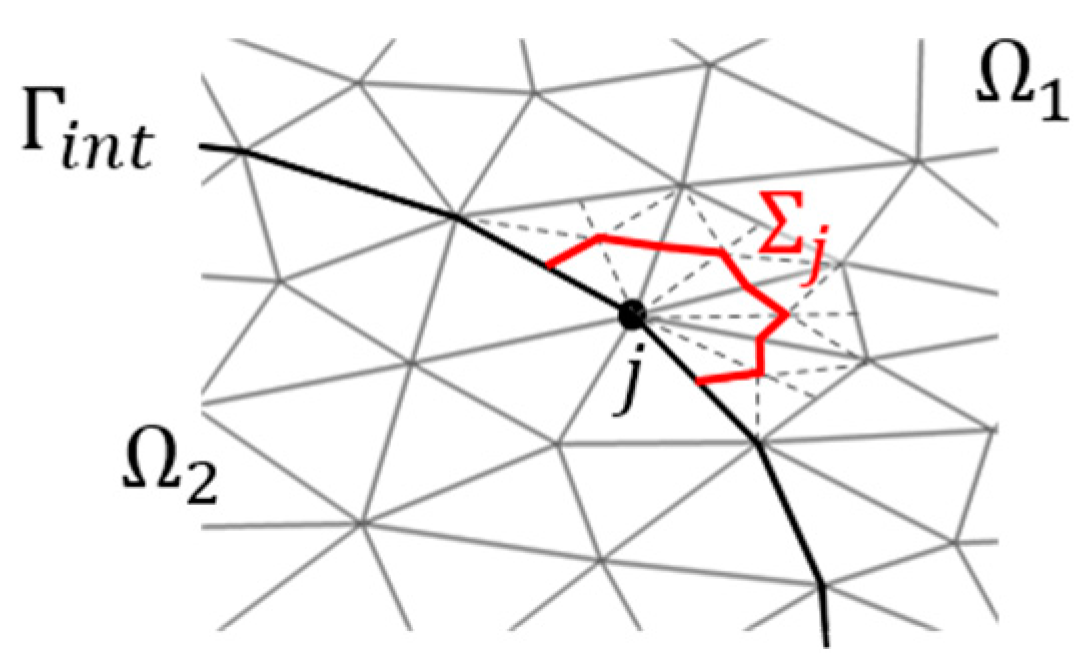
It is demonstrated in [10] that this term corresponds physically to the inward flux of across the “box” associated with node in the dual mesh obtained from the barycentric subdivision of the primal 2D mesh. In particular, at a node belonging to the discretization of the interface between and , the quantity is interpreted as the flux through the “cap” , as shown in Figure 2.
However, this interpretation is only valid for first-order elements, and it is not the case of higher-order elements where it is a mere mathematical equivalent variable. Yet, this variable obeys a continuity condition across the interface, as will be shown in Section 2.2. Parameters are used here instead of the approximation of the normal derivative that is normally present in the classical boundary element method [3].
As in the standard BEM, the 2D fundamental solution of Laplace’s equation is exploited in order to eliminate the domain integral. Let us recall that it is obtained from the equation
where is the Dirac delta function at any point (Figure 1).
A FEM solution exists [6,7], and is readily derived from the Galerkin problem associated with the formulation (7):
where the FEM solution is interpolated as
An illustrative example of the FEM solution of a Green’s function on an arbitrary domain is given in Figure 3.
In the same way as for given by (6), we can write the nodal approximation:
Note that , as a consequence of Gauss’s law for any internal node of the mesh . If we combine Equations (3)–(6) and (9), a little algebra suffices to show that:
By performing integration of the source term, (11) becomes:
where is the set of triangles of the source region sharing the node and denotes the area of the triangle.
Conversely, using (4), adapted to and Equation (10) instead of (6), we can easily write:
Now, by equating (12) to (13), we can write the following expression:
where the domain contribution is eliminated as announced previously, and has been replaced by since it is now licit to extend the outer boundary at infinity. Equation (14) can be regarded as a discrete equivalent of Green’s second identity that has been derived directly from the Galerkin approach.
Henceforth, it is necessary to write (14) for all the nodes belonging to the boundary , in order to derive a consistent linear system of equations. However, due to the singularity of the function, the boundary condition of the problem (7) must be changed as:
so that the Galerkin formulation (8) is replaced by:
where is the common Kronecker symbol and is the classical geometric factor of standard BEM, i.e., it is equal to the ratio , where is the internal (with respect to the FEM region ) angle at node [3]. It is easy to show that, in the FEM-Green context:
that can again be interpreted as Gauss‘s law at the discrete level. Finally, the FEM-Green scheme leads to the system of the simultaneous equations:
where potential and flux values are the unknown parameters along the interface .
At this point, the solution of (18) requires the computation of the FEM approximations that is highly time consuming and does not make sense since is unbounded in the context of open boundary problems. Then, coefficients and are modified by using the exact fundamental solutions instead of . More precisely the following interpolant should be considered:
where is the distance between nodes and . However, the infinite value must be replaced by a value that can be derived from the discrete Gauss’s law (17), i.e.,
and:
Parameter can be considered as an estimate of the geometric factor described above. By eliminating this parameter between Equations (20a) and (20b), after some algebra that we skip for the sake of conciseness, we obtain the expression of :
As outlined above, meshing the whole domain is not a necessity since the internal nodes are not involved in (18). In fact, that would not make sense since this outer region is unbounded. A single layer of finite elements along the boundary (in gray in Figure 1) is sufficient. Any internal mesh of is used for field calculation at a postprocessing step.
By comparing with the implementation of the boundary element method, no cumbersome analytical or numerical (Gaussian quadrature) integration is required to compute the coefficients , and of (18) so that an obvioussignificant reduction of the computational burden is expected. However, the computational effort to build the linear system (18) still scales as as in classical BEM.
Lastly, note that the method can be applied to axisymmetrical problems where the fundamental solution is based on a complete elliptic integral of the first kind as it was shown by the author in [5].
2.2. FEM/FEM-Green Coupling
A complete set of equations associated with the hybrid FEM/FEM-Green is necessary to solve the whole problem. Then, the Galerkin problem related to the finite element domain has now to be derived. By referring again to Figure 1 and Equation (1b), the governing equation is either:
for general nonlinear magnetostatic problems, or
in case of time-harmonic eddy-current problems.
The FEM problem is given by the respective Galerkin formulations
and
The Galerkin equation written for a node belonging to the interface in a conventional FEM method would be:
The right-hand side of (25) vanishes for nodes that are not adjacent to the source region . By introducing the expression (6) of , Equation (25) becomes:
Finally, a global system of algebraic equations of the whole problem is obtained by an assembling procedure of Equations (18) and (24), or (25), and (27). It may be expressed as the partitioned matrix form:
where the unknown vector refers to the nodal flux values on , and vectors and are related to the nodal potential values on and , respectively. Submatrices and represent the FEM-Green equations with the entries and , or , respectively. The submatrix comes from the FEM contribution and is a unit matrix induced by (27). As it is the case for most FEM/BEM coupling methods, the global matrix has no particular structure, i.e., it is neither symmetric, nor positive definite. However, the G submatrices are symmetric. A general solver must be used for the solution of the system (28), but the optimization of this specific point has not been investigated in the paper. Finally, vector relates to the source excitation that appears in the right-hand side of (18) and (27).
3. Numerical Results
The method has been applied to two magnetic problems to estimate the performance of our numerical scheme. In the first example, a comparison with the classical FEM/BEM technique and the FEM with a large truncated outer boundary has been carried out to assess the accuracy of the method. As in previous papers of the author [4,5], all the algorithms were implemented in the MATLAB® environment on a standard desktop computer. The LU-decomposition was used for the solution of the involved linear systems. COMSOL Multiphysics® software has been used for the generation of the various meshes required by the simulations and also in order to confirm the results obtained by the FEM.
3.1. Example 1–A Nonlinear Magnetostatic Problem
The first example is a 2D nonlinear magnetostatic problem defined on a C-shaped magnetic circuit with an excitation coil ( A/m2) in air region , as depicted in Figure 4.
As an illustration, a magnetic field plot obtained by using COMSOL Multiphysics® is given in Figure 5. As classical FEM is used, the problem is encased in a circular box with a radius equal to about 15 times the mean size of the device. Magnetic induction along the line AB crossing the air gap, as shown in Figure 5, is plotted for the three methods in Figure 6. It is clear that FEM/BEM and FEM/FEM-Green methods are both in excellent agreement. Table 1 presents the magnetic energy restricted in an arbitrary rectangular domain of size 0.6 × 0.4 m centered on the origin of the reference frame of the geometry and computed at a postprocessing step for both FEM/BEM and FEM/FEM-Green techniques. The number of elements of magnetic and coil regions , is taken as a parameter. Convergence is observed and an extremely good agreement is obtained between the methods. A value of 74.53 J/m has been obtained with COMSOL in the same domain, by using a supplementary large external bounding rectangular box of size 10 × 10 m. This result is in coherence with our results.
As already emphasized in [5], there is a lower computational burden in the FEM-Green part of the system (28), compared with the equivalent BEM part. However, global CPU times measured for both methods for the proposed example are not vastly different due to the important part involved in the solutions of the system at every iteration.
3.2. Example 2–Eddy-Currents in a Conducting Magnetic Region
The second example deals with a conducting region made of copper ( H/m and S/m) and driven by source currents ( A/m2, frequency 5 Hz) located in region , embedded in air region , as presented in Figure 7.
Time-harmonic modified Helmholtz equation is applied to this problem. COMSOL Multiphysics® solution is also given in Figure 7 where the induced current density is given by the statement:
Real and imaginary parts of along the line AB crossing the conducting region is plotted in Figure 8 for FEM and FEM/FEM-Green methods (FEM-BEM is not applied here).
There is an excellent agreement between the results as the symbols and match the curves extremely well. The simulation has been realized with the number of triangular elements in conducting and source regions equal to 5811 as depicted in Figure 7.
The losses have also been computed. A total of 9.45 mW/m has been obtained with the same mesh. This value should be compared with the value 9.42 mW/m computed with FEM and a circular box with a radius equal to about 100 times the mean size of the device. Those global quantities are quite similar considering the approximations that have been adopted.
3.3. Discussion
As a general comment about our method, some simulations have been carried out with a larger inside/outside interface around the active region, i.e., the magnetic circuit in the first example, eventually by including the excitation inside the FEM part. The same tests have been realized with the conducting part in the second example. The results are extremely close to each other in both cases.
However, we notice experimentally that it seems that a regular mesh with a single layer of triangle between the active (FEM) and outside parts gives a better accuracy of the method. Then, some precautions should be taken into account when preparing the mesh with our method. This is a constraint in our method that should be carefully considered at the programming stage.
4. Conclusions
The FEM/FEM-Green method presented in this paper has been proposed as an alternative to the classical FEM/BEM methods for the treatment of magnetic open boundary problems. The FEM-Green formulation applied to the open region is obtained by using the FEM approximation of fundamental solutions that leads to a discrete equivalent of the second Green’s identity. The coupling with the finite element method used for the inner domains appears to be natural due to the same Galerkin approach in both mathematical treatments. Numerical results have pointed out an extremely good agreement between our technique and the standard hybrid FEM/BEM coupling that has been implemented for the sake of comparison. The advantages of the FEM-Green approach are an easier implementation since no particular integration is involved in the computation of the matrix coefficients, the absence of the somewhat awkward normal derivative of the fundamental solution in the formulation, and a more natural coupling with FEM. However, a layer of finite element mesh is required around the inner parts, and it should be carefully taken into account when programming the method. Our numerical scheme can be theoretically extended to 3D problems in the case of scalar potential applications (electrostatics, magnetostatics with scalar magnetic potential), and higher-order (e.g., quadratic) elements. In the latter case, there is no obvious geometrical interpretation of the nodal flux as with linear triangles, but it remains a representative variable. These aspects should be investigated in future work.
Funding
This research received no external funding.
Institutional Review Board Statement
Not applicable.
Informed Consent Statement
Not applicable.
Data Availability Statement
Not applicable.
Conflicts of Interest
The author declares no conflict of interest.
References
- Chen, Q.; Konrad, A. A Review of Finite Element Open Boundary Techniques for Static and Quasi-Static Electromagnetic Field Problems. IEEE Trans. Magn. 1988, 24, 80–85. [Google Scholar] [CrossRef]
- Stephan, E.P. Coupling of Boundary Element Methods and Finite Element Methods. In Encyclopedia of Computational Mechanics Fundamentals, 2nd ed.; Stein, E., de Borst, R., Hughes, T.J.R., Eds.; John Wiley & Sons: Hoboken, NJ, USA, 2004; Volume 2, pp. 375–412. [Google Scholar] [CrossRef]
- Brebbia, C.A.; Telles, J.F.C.; Wrobel, L.C. Boundary Element Techniques, Theory and Applications in Engineering; Springer: Berlin, Germany, 1984; pp. 400–426. [Google Scholar] [CrossRef]
- Lobry, J. New boundary element formulation for the solution of Laplace’s equation. In Boundary Elements and Other Mesh Reduction Methods XLII; Cheng, A.H.D., Tadeu, A., Eds.; WIT Trans. Eng. Sci.: Southampton, UK, 2019; Volume 126, pp. 63–73. [Google Scholar] [CrossRef] [Green Version]
- Lobry, J. A New FEM–BEM Coupling for the 2-D Laplace Problem. IEEE Trans. Magn. 2021, 24, 80–85. [Google Scholar] [CrossRef]
- Hartmann, F. Green’s Functions and Finite Elements, 1st ed.; Springer: Berlin, Germany, 2013; pp. 109–208. [Google Scholar] [CrossRef]
- Araya, R.; Behrens, E.; Rodriguez, R. A posteriori error estimates for elliptic problems with Dirac delta source terms. Numerische Mathematik 2006, 105, 193–216. [Google Scholar] [CrossRef]
- Zienkiewicz, O.; Lyness, J.; Owen, D. Three-dimensional magnetic field determination using a scalar potential—A finite element solution. IEEE Trans. Magn. 1977, 13, 1649–1656. [Google Scholar] [CrossRef]
- Chari, M.V.K.; Salon, S.J. Numerical Methods in Electromagnetism; Academic Press: San Diego, CA, USA, 1999; pp. 143–349. [Google Scholar] [CrossRef]
- Bossavit, A. How Weak is the Weak Solution in Finite Element Methods? IEEE Trans. Magn. 1998, 35, 2429–2432. [Google Scholar] [CrossRef]
Figure 1.
General configuration for the 2D modified Helmholtz problem and the FEM/FEM-Green treatment.
Figure 1.
General configuration for the 2D modified Helmholtz problem and the FEM/FEM-Green treatment.

Figure 2.
Typical finite element triangular mesh and barycentric “cap” for an interface node j.

Figure 3.
Example of the FEM discretization of a Green’s function on a domain Ω.

Figure 4.
C-shaped magnetic circuit: mesh for FEM/FEM-Green treatment and B-H curve of the magnetic core material.
Figure 4.
C-shaped magnetic circuit: mesh for FEM/FEM-Green treatment and B-H curve of the magnetic core material.

Figure 5.
Plot of magnetic induction (in teslas) and field lines provided by COMSOL Multiphysics® package. Coordinate dimensions are in meters.
Figure 5.
Plot of magnetic induction (in teslas) and field lines provided by COMSOL Multiphysics® package. Coordinate dimensions are in meters.

Figure 6.
(a): Plot of magnetic vector potential (Wb/m) and (b) plot of magnetic induction (T) along the line AB for FEM (solid line), FEM/BEM (red stars) and FEM/FEM-Green (blue circles) methods. Abscissa in meters.
Figure 6.
(a): Plot of magnetic vector potential (Wb/m) and (b) plot of magnetic induction (T) along the line AB for FEM (solid line), FEM/BEM (red stars) and FEM/FEM-Green (blue circles) methods. Abscissa in meters.

Figure 7.
Eddy-current problem: mesh and results.

Figure 8.
Plot of induced current density (A/m2) along line AB, obtained with FEM and FEM/FEM-Green methods. Abscissa in meters.
Figure 8.
Plot of induced current density (A/m2) along line AB, obtained with FEM and FEM/FEM-Green methods. Abscissa in meters.


Table 1.
Magnetic energy (J/m) in an embedding rectangular box vs. the number m of elements of the magnetic and coil regions.
Table 1.
Magnetic energy (J/m) in an embedding rectangular box vs. the number m of elements of the magnetic and coil regions.
| m | FEM/BEM | FEM/FEM-Green |
|---|---|---|
| 3204 | 76.33 | 75.35 |
| 4938 | 74.61 | 74.33 |
| 19,752 | 74.49 | 74.42 |
| 50,048 | 74.54 | 74.86 |
Publisher’s Note: MDPI stays neutral with regard to jurisdictional claims in published maps and institutional affiliations. |
© 2021 by the author. Licensee MDPI, Basel, Switzerland. This article is an open access article distributed under the terms and conditions of the Creative Commons Attribution (CC BY) license (https://creativecommons.org/licenses/by/4.0/).
Share and Cite
MDPI and ACS Style
Lobry, J. A FEM-Green Approach for Magnetic Field Problems with Open Boundaries. Mathematics 2021, 9, 1662. https://0-doi-org.brum.beds.ac.uk/10.3390/math9141662
AMA Style
Lobry J. A FEM-Green Approach for Magnetic Field Problems with Open Boundaries. Mathematics. 2021; 9(14):1662. https://0-doi-org.brum.beds.ac.uk/10.3390/math9141662
Chicago/Turabian StyleLobry, Jacques. 2021. "A FEM-Green Approach for Magnetic Field Problems with Open Boundaries" Mathematics 9, no. 14: 1662. https://0-doi-org.brum.beds.ac.uk/10.3390/math9141662
Note that from the first issue of 2016, this journal uses article numbers instead of page numbers. See further details here.