
On the Loop Homology of a Certain Complex of RNA Structures


1
Biocomplexity Institute and Initiative, University of Virginia, Charlottesville, VA 22904-4298, USA
2
Mathematics Department, University of Virginia, Charlottesville, VA 22904-4137, USA
*
Author to whom correspondence should be addressed.
†
Physical Address: Biocomplexity Institute, Town Center Four, 994 Research Park Boulevard, Charlottesville, VA 22911, USA.
‡
Mailing Address: Biocomplexity Institute, P.O. Box 400298, Charlottesville, VA 22904-4298, USA.
Mathematics 2021, 9(15), 1749; https://0-doi-org.brum.beds.ac.uk/10.3390/math9151749
Submission received: 15 June 2021
/
Revised: 8 July 2021
/
Accepted: 21 July 2021
/
Published: 24 July 2021
(This article belongs to the Special Issue Discrete and Algebraic Mathematical Biology)
Abstract
:In this paper, we establish a topological framework of -structures to quantify the evolutionary transitions between two RNA sequence–structure pairs. -structures developed here consist of a pair of RNA secondary structures together with a non-crossing partial matching between the two backbones. The loop complex of a -structure captures the intersections of loops in both secondary structures. We compute the loop homology of -structures. We show that only the zeroth, first and second homology groups are free. In particular, we prove that the rank of the second homology group equals the number of certain arc-components in a -structure and that the rank of the first homology is given by , where is the Euler characteristic of the loop complex.
1. Introduction
Ribonucleic acid (RNA) is a biomolecule that folds into a helical configuration of its primary sequence by forming hydrogen bonds between pairs of nucleotides. The most prominent class of coarse-grained structures are the RNA secondary structures [1,2]. These are contact structures that can be represented as diagrams where vertices are nucleotides and arcs are base pairs drawn in the upper half-plane. As a secondary structure can be uniquely decomposed into loops, the free energy of a structure is calculated as the sum of the energy of its individual loops [3]. The loop-based energy models for RNA secondary structure prediction have played an important role in unveiling the various regulatory functions of RNA [4].
RNA molecules evolve under selection pressures on both sequence and structure. One prominent example are RNA riboswitches [5], which is a class of RNA molecules that can express two alternative secondary structures, each of which appears in a specific biophysical context. In order to analyze riboswitch sequences, Huang et al. developed a Boltzmann sampler of sequences that are simultaneously compatible with a pair of structures, i.e., a bi-secondary structure, based on the loop energy model [6]. The time complexity of computing such bi-compatible sequences turns out be intimately related to the number of so called exposed nucleotides, i.e., the number of vertices shared by multiple loops appearing in the algorithm. In some sense, finding bi-compatible sequences is easy if the intersection of such loops is small and becomes difficult when the intersection is large. In order to address the complexity problem, Bura et al. studied the simplicial homology of the loop complex (derived from the intersections of loops) of a bi-secondary structure [7,8]. Subsequently, they introduced the weighted homology of bi-structures, in which simplices are endowed with specific weights allowing the expression of the size of the loop intersections [9].
The aforementioned work focuses on the structural transition without changing the underlying sequence. However, selection pressures act on both sequence and structure, resulting in the simultaneous change of genotypes and phenotypes. This motivates the study of the evolutionary transition between two distinct sequence–structure pairs. In what follows, we take the first step by, analogous to [7,8], computing the simplicial homology of their loop complex.
In this paper we study triples, , consisting of an ordered pair of RNA secondary structures, , [1,2,10,11,12,13] together with a non-crossing partial matching, , between the two backbones. We shall denote such a triple a transition structure or τ-structure and note that the mapping relates homologous bases between two underlying RNA sequences.
The topological framework of -structures developed here is designed to quantify the probability of evolutionary transitions between RNA sequence-structure pairs subject to specific sequence constraints. In an algorithmic guise, -structures play a central role in solving the following computational problem: Given two arbitrary RNA secondary structures, determine a pair of specifically related sequences that minimizes the total free energies of the two sequence–structure pairs. Our main objective is to compute the simplicial homology of the loop complex of a -structure. In order to state our main theorem, we next introduce the notions of -crossing and arc-component.
Two arcs and are -crossing, i.e., if either one of the following is the case:
- (1)
- Both and are incident to -arcs such that or , or;
- (2)
- Both and are incident to -arcs such that or .
-crossing induces an equivalence relation for which nontrivial equivalence classes are called arc-components. An arc-component is of type 1 if both endpoints of any arc are incident to -arcs.
We shall prove the following main result.
Main Theorem.
Let be a τ-structure and the n-th homology group of its loop complex, . Then, the following is the case:
where γ denotes the number of arc-components of type 1 and χ the Euler characteristic of .
Our framework generalizes the work of [7,8] on bi-structures. Bi-structures can be viewed as particular -structures, namely those over two identical sequences. The loop complex of a bi-structure exhibits only a nontrivial zeroth and second homology, the latter being freely generated by crossing components [7,8]. On the algorithmic side, -structures play a similar role as bi-structures in [6] where a Boltzmann sampler of sequences that are simultaneously compatible with two structures is presented.
The loop complex of -structures exhibits a variety of new features. First it has in general a nontrivial first homology group. Secondly, it features two types of arc-components: Those of type 1, which correspond to spheres, and arc-components of type 2, which correspond to surfaces with a nontrivial boundary (see Section 7).
In order to prove the main theorem, we first establish basic properties of the loop complex . Secondly, we manipulate X by means of simplicial collapses and then dissect , which is a certain sub-complex of dimension one. As a result, we derive , which is a specific X-sub-complex, and we organize it into its crossing components. We note that is not unique, as its construction depends on certain choices. We then proceed with a combinatorial analysis of -crossing components, which lays the foundation for proving that their geometric realizations are either spheres or surfaces with boundary.
The combinatorics of crossing components, specifically Lemma 6, further controls the manner crossing components are glued and this observation facilitates to prove the main result in two stages. First, by computing the homology of components in isolation and, secondly, by computing the homology of the loop complex by Mayer–Vietoris sequences. Several of our arguments are reminiscent of ideas of classical facts, for instance the Jordan curve theorem in the proof of Lemma 7.
The paper is organized as follows: In Section 2, we recall the definitions of RNA secondary structures, bi-structures and their loop complexes. In Section 3, we introduce -structures and present some basic facts of their loop complexes. In Section 4, we simplify the loop complex in multiple rounds via simplicial collapses and topological stratification. In Section 5, we investigate the combinatorics of crossing components in the simplified complex. We then compute the homology of components in Section 6 and integrate this information in order to obtain the homology of -structures in Section 7. Finally we discuss our results in Section 8.
2. Secondary Structures, Bi-Structures and the Loop Complex
An RNA secondary structure encapsulates the nucleotide interactions within a single RNA sequence. It can be represented as a diagram, which consists of a labeled graph over the vertex set for which the vertices are arranged in a horizontal line and arcs are drawn in the upper half-plane. Each vertex corresponds to a nucleotide in the primary sequence and each arc, which is denoted by , represents the base pairing between the i-th and j-th nucleotides in the RNA structure. Two arcs and are crossing if . An RNA secondary structure is defined as a diagram satisfying the following three conditions [1,2]: (1) if is an arc, then ; (2) any two arcs do not have a common vertex; (3) any two arcs are non-crossing.
Given a secondary structure S, the set is called the backbone and an interval denotes the set of consecutive vertices . A vertex k is covered by an arc if and there exists no other arc such that . The set of vertices covered by an arc is called a loop, s, and we refer to as the covering arc of s. We shall equip each diagram with two “formal” vertices at positions 0 and together with the arc , which we call the rainbow. Its associated distinguished loop is called the exterior loop. Each loop, s, can be represented as a disjoint union of intervals on the backbone of S, , such that and for form arcs and any other vertices in s are unpaired. By construction, a diagram S is in one-to-one correspondence with its set of arcs as well as its set of loops .
Let be a collection of finite sets. A subset is defined to be a d-simplex of if the set intersection . Let be the set of all d-simplices of . The nerve of is a simplicial complex given by .
The nerve formed by the collection of S-loops is referred to as the loop complex of a secondary structure S. The fact that secondary structures correspond to non-crossing diagrams immediately implies that the loop complex of a secondary structure is a tree.
Let S and T be two secondary structures. The pair of secondary structures S and T over , , is called a bi-structure. We represent a bi-structure as a diagram on a horizontal backbone with the S-arcs drawn in the upper and the T-arcs drawn in the lower half plane. The nerve formed by S-loops and T-loops of a bi-structure, R, is called the loop complex, .
In bi-structures [7], two arcs are equivalent if there exists a sequence of arcs such that two consecutive arcs and are crossing for . A crossing component of is an equivalence class that contains at least two crossing arcs.
The loop complex of a bi-structure has a nontrivial zeroth and second homology group. In particular, the first homology is zero and the second homology is free and its rank equals the number of crossing components of the bi-structure R [8].
3. Some Basic Facts
Let S and T be two secondary structures over and , respectively. We shall refer to their backbones as and . We refer to the pair as a ϕ-arc between and . Two -arcs and are crossing if and .
Definition 1.
A-structure I is a triple consisting of an ordered pair of secondary structures, , together with a partial matching ϕ between their vertex sets and such that any two ϕ-arcs are non-crossing.
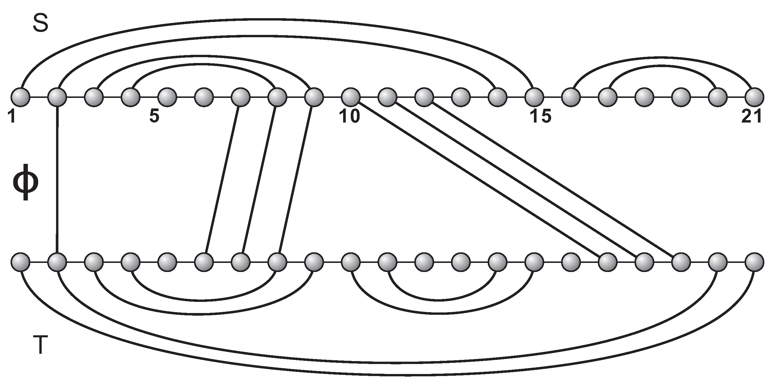
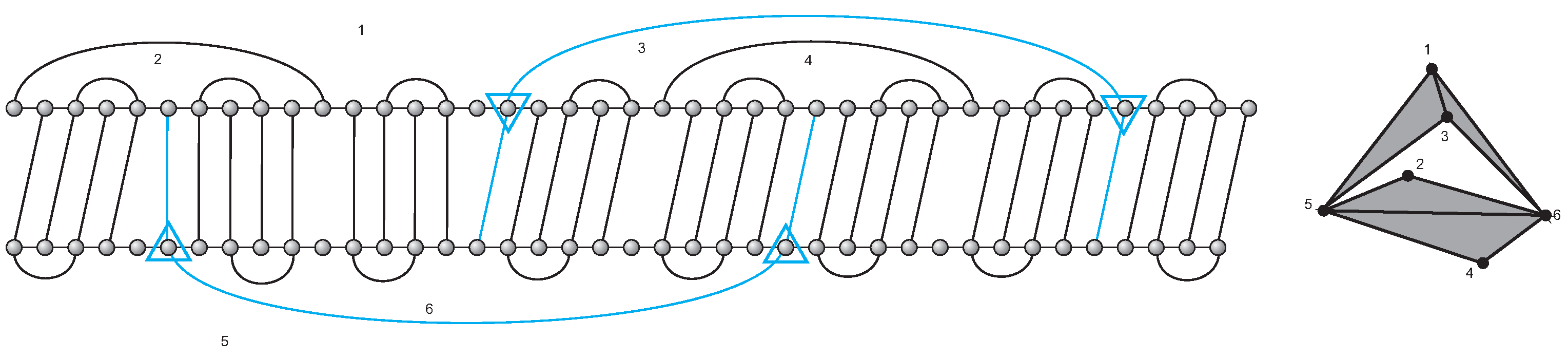
In analogy to the case of bi-structures, we shall represent the diagram of a -structure as a labeled graph over two horizontal backbones in which S-arcs are drawn in the upper halfplane and T-arcs are drawn in the lower halfplane with the edges drawn in between the two backbones representing (see Figure 1).
A bi-structure corresponds to a particular -structure having two backbones of the same length and being the identity map.
The partial matching induces an equivalence relation ∼ on the set of vertices of the two backbones by identifying for each pair the vertices i and . The -arcs then correspond one-to-one to nontrivial equivalence classes of size two. This equivalence relation gives rise to the definition of a loop in a -structure.
Definition 2.
Given a S-vertex or T-vertex , anI-vertex, , is an equivalence class induced by v, i.e., . Given an S-loop s, the -loop is the set of equivalence classes induced by the set of s-vertices. Similarly, we define the -loop. AnI-loopis defined to be either an -loop or a -loop.
Now we are in position to introduce the loop complex of a -structure.
Definition 3.
The nerve formed by I-loops is called the loop complex, where denotes the set of d-simplices, i.e., the non-empty intersections of d distinct loops. shall denote the n-th homology group of the loop complex of I.
Let us proceed by collecting some basic properties of the loop complex.
Proposition 1.
Let be a τ-structure and be two distinct S-vertices. Then . In particular there exists a bijection between vertices in an S-loop s and vertices in the corresponding -loop .
Proof.
By definition, any two -arcs in the partial matching do not share common endpoints. Thus, maps and to different T-vertices. Therefore the equivalence classes and are different. □
Proposition 2.
Let be a τ-structure and , be three different -loops. Then, it follows that:
- (1)
- either or ;
- (2)
- .
Proof.
For the secondary structure S, any two S-loops and either have trivial intersection or intersect at two endpoints of one arc, i.e., either or . Proposition 1 guarantees that , whence assertion . Any S-vertex is contained in at most two distinct S-loops. Thus . By Proposition 1, . □
By abuse of notation, we refer to -loops and -loops simply as S-loops and T-loops , respectively.
Proposition 3.
Let I be a τ-structure with loop complex . Then, any 2-simplex has the form or , where are S-loops and are T-loops.
Proof.
By construction, the three loops in a 2-simplex have a non-empty intersection. In view of Proposition 2, not all three loops are from the same secondary structure. Therefore, is of the form or . □
A 1-simplex is called pure if both and belong to the same secondary structure and mixed. Proposition 3 shows that any 2-simplex contains exactly one pure edge and two mixed edges.
Proposition 4.
Let I be a τ-structure with loop complex . Then, any 3-simplex has the form , where are S-loops and are T-loops.
Proof.
Suppose that . As a face of , . By Proposition 3, we can w.l.o.g. set that , and . Similarly, the face implies that is necessarily a T-loop, i.e., . □
Definition 4.
Given a simplex , a face is called-free if, for any simplex containing ω, is a face of σ. Clearly, σ is maximal in . Moreover, σ is the unique maximal simplex that contains ω.
Proposition 5.
Let I be a τ-structure with loop complex . Then, any 3-simplex contains a σ-free, mixed 1-face ω.
Proof.
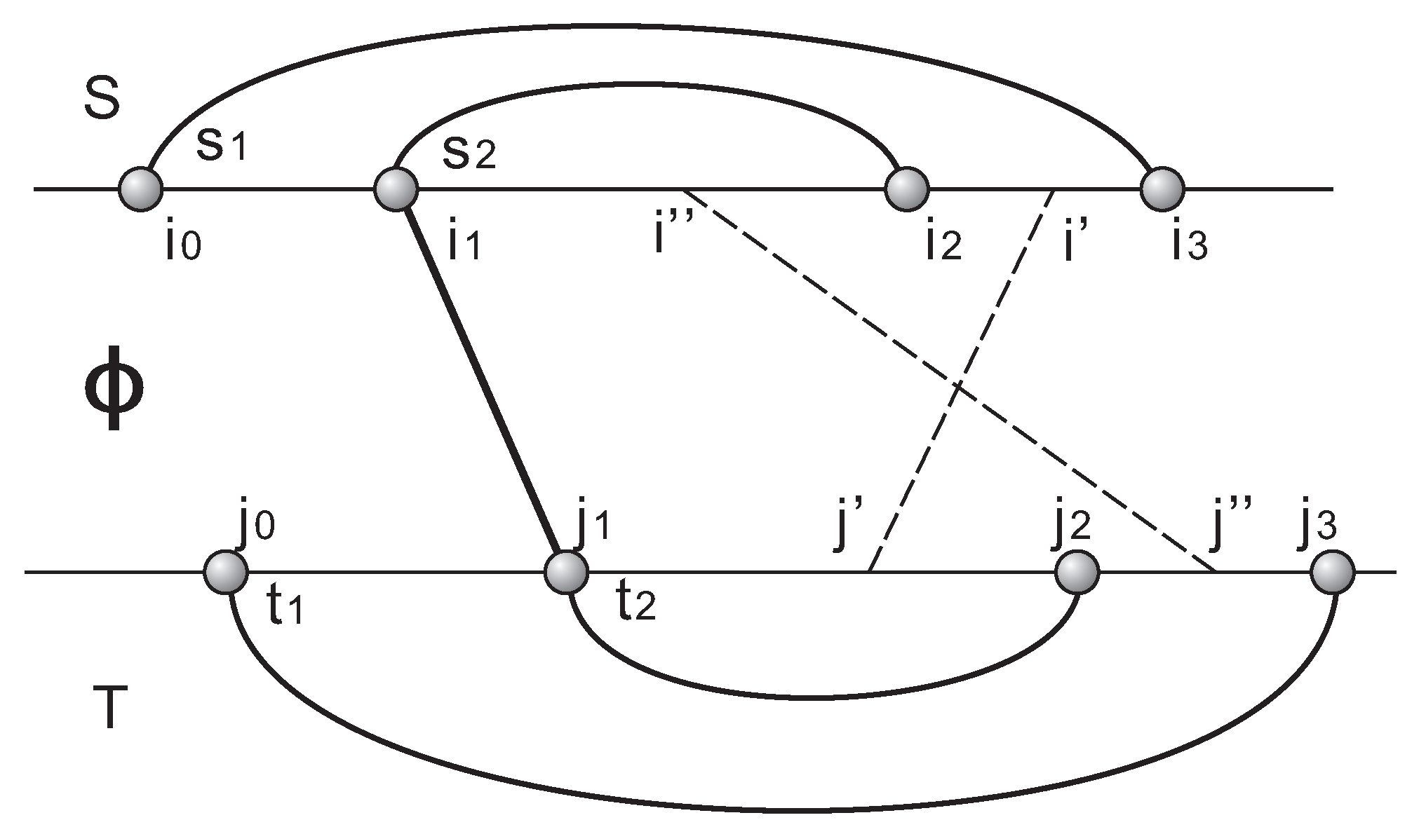
Let . Suppose that the covering arcs of the loops are , , and , respectively, and that we have the distinguished -arc with . Then, the loops intersect at the equivalence class of and by w.l.o.g. we may assume and (see Figure 2).
We shall prove the proposition by contradiction. Suppose that none of the mixed 1-faces of are free, we consider the two particular mixed edges and . By assumption, there exist 2-simplices and , such that and , neither of which are faces of .
In view of , it follows from Proposition 3 that is of the form or . By w.l.o.g. we set . Since , we have . By construction, . It implies that there exists an I-vertex , which corresponds to a -arc . As and , the -arc is distinct from . Since , the -arc connects two intervals and , i.e., and . Note that if , then and , i.e., the -arcs and are crossing, which is a contradiction. Hence, we derive that the -arc connects and (see Figure 2).
Similarly, corresponds to a -arc distinct from . Since , it follows that the -arc connects two intervals and (see Figure 2). In view of and , the -arcs and are crossing, which contradicts the fact that -arcs are non-crossing.
Accordingly, the non-crossing property of -arcs implies that either one, or , is -free. □
Proposition 6.
Given a loop complex , then any 3-simplex contains at least two σ-free 2-faces.
Proof.
By Proposition 5, contains at least one -free mixed edge . Let and denote the 2-faces of containing . Suppose that there exists a simplex satisfying and . Then also contains , which contradicts being -free. Therefore, is -free and, analogously, we derive that is -free. □
Proposition 7.
Let I be a τ-structure with loop complex . Then and for .
Proof.
By assumption, induces at least one -arc, which in turn gives rise to at least a 1-simplex connecting an S-loop and a T-loop. Therefore, is path-connected and . By the pigeonhole principle, for any set of I-loops with , at least three belong to the same secondary structure. By Proposition 2, these three loops intersect trivially. Thus, for , the intersection of any loops is trivial. As a result, does not contain simplices of dimension four or higher. Therefore, and for . □
4. From to
We now begin computing the homology of the loop complex of a -structure. Directly constructing its discrete Morse function [14,15] or gradient vector field seems rather involved. We shall take a slightly different approach along the lines of discrete Morse theory. We shall simplify the loop complex in multiple rounds and render it amendable to its homological analysis. One of these simplifications is obtained via elementary collapses, which is a reduction introduced by J.H.C. Whitehead [16]. These collapses can be understood in terms of non-critical points of the Morse function.
4.1. Simplicial Collapses
The notion of elementary collapse is closely related to the freeness of a simplex. Given a complex K, let be a maximal simplex and be a -free face with codimension 1. The removal of and constitutes elementary collapse [16,17] and gives rise to a new complex . We say that K simplicial collapses to a sub-complex , which is denoted by if there is a sequence of complexes such that is obtained from via an elementary collapse. Clearly, K and are homotopy equivalent.
In the following, we shall employ simplicial collapses in order to reduce the loop complex in two steps: first, eliminating all tetrahedra and then removing triangles possessing a free edge.
Step 1: Given a 3-simplex , Proposition 5 guarantees that always has a free mixed edge and two free triangles containing . The triple is called a -butterfly. In analogy to the analysis in case of bi-structures [7], we perform the butterfly removal on the loop complex. Specifically, the simplicial collapse consists of two elementary collapses with respect to and and provides us a sub-complex , which is homotopy equivalent to .
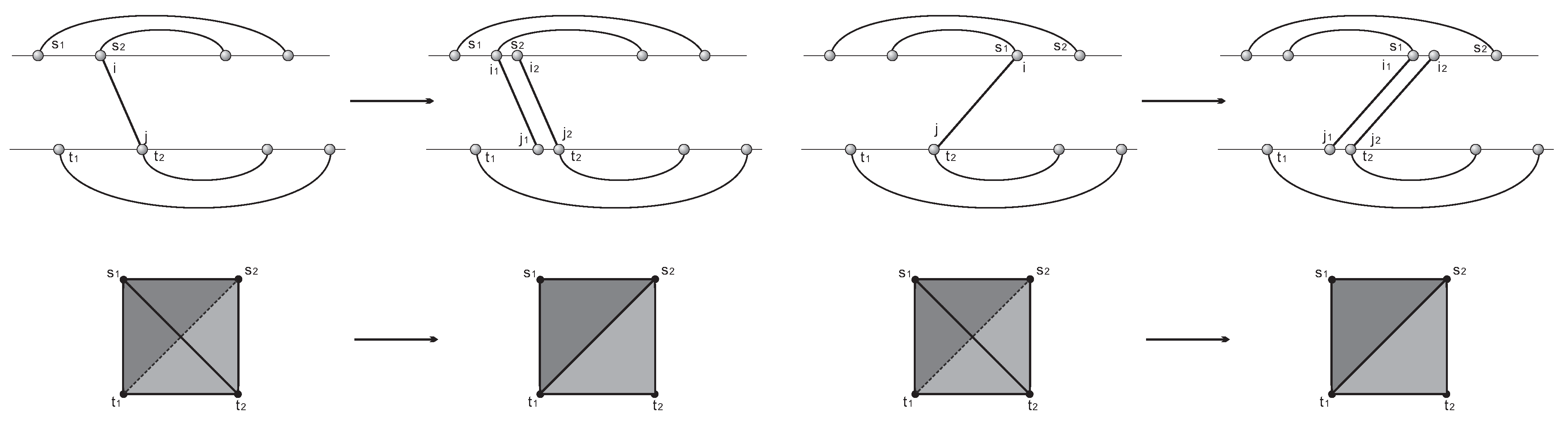
We observe that is again the loop complex of a -structure obtained by splicing vertices in I as follows: For any I-vertex , suppose that q is the equivalence class of an S-vertex i and a T-vertex j. Then, there is a -arc connecting i and j, i.e., . We now splice i into two consecutive vertices and splice j into two consecutive vertices . The -arc is replaced with two new -arcs and . The arcs are connected in a manner such that the mixed edge is not formed in . In the case of , we depict the resulting -structure in Figure 3 and note that all other cases are treated similarly. Furthermore, we remove any other -arcs that give rise to , or . It is straightforward to verify that the loop complex of is exactly .
By iteratively eliminating all 3-simplices, and the associated -butterflies, we derive a sequence of sub-complexes such that X does not contain any 3-simplices. Accordingly, we obtain a sequence of -structures by splicing the corresponding vertices of such that the loop complex of is given by . It is clear that the sub-complex X satisfies the following property.
Lemma 1.
Let be the loop complex of a τ-structure I and X be the complex obtained by removing from all 3-simplices σ and the associated σ-butterflies. Then the following is the case:
- (1)
- X is the complex of a τ-structure such that each ϕ-arc is incident to at most one arc;
- (2)
- X is a sub-complex of such that the 0-th skeleton and X does not contain any 3-simplices;
- (3)
- , for .
A complex possessing the properties of Lemma 1 is called lean. As an immediate consequence we obtain the following.
Corollary 1.
Let I be a τ-structure, then .
Proof.
In view of Proposition 1, as a sub-complex of , X does not contain any 3-simplices. For X holds , whence . □
Step 2: Suppose that is a 2-simplex in X having a free 1-face . By collapsing , we obtain a sub-complex . By successively deleting 2-simplices together with -free edges, we derive a sequence of sub-complexes such that each 2-simplex of does not contain any free 1-face.
Proposition 8.
Let be a complex obtained from X by iteratively removing all 2-simplices ω together with τ-free 1-face. Then, the following is the case:
- (1)
- is a sub-complex of X such that the 0-th skeleton and each 2-simplex of does not have a free 1-face;
- (2)
- For , we have .
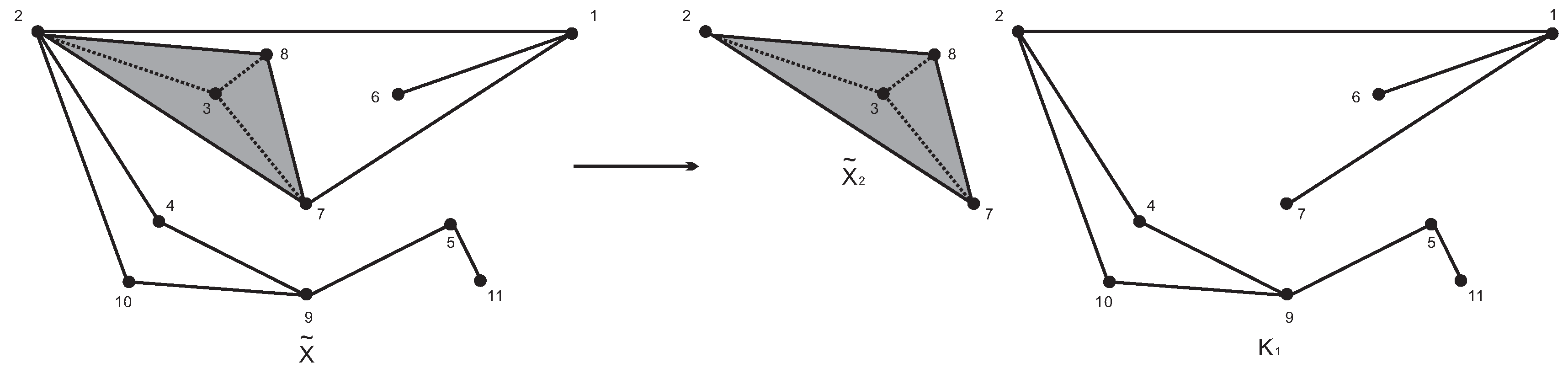
Figure 4 displays the simplicial collapse from X to .
Remark 1.
The sub-complex is not unique. By construction, depends on the particular sequence of the simplicial collapses, as well as which free face of a simplex is being removed (see Figure 5)
Lemma 1 guarantees that is derived from a lean complex.
Lemma 2.
Let be the sub-complex derived from a lean complex, then the following is the case:
- (1)
- For any 2-simplex , holds , i.e., any 2-simplex Δ corresponds to the ϕ-arc, ;
- (2)
- Any pure 1-simplex ω of is either maximal or contained in exactly two 2- simplices . In the latter case, ω is associated with an arc in I, such that vertices are incident to ϕ-arcs and , respectively.
Proof.
For any , we have . By construction, in , is not -free, whence there exists another 2-simplex containing . Lemma 1 guarantees that does not contain any 3-simplices, i.e., we have the following.
Therefore, sets and are disjoint and both have cardinality 1, whence assertion (1) follows. Let , then is in one-to-one correspondence with the vertex i as well as its induced -arc in I.
Suppose the pure 1-simplex is not maximal, then there exists at least one 2-simplex having as a face. Since we work in the complex , cannot be -free, whence there exists another 2-simplex containing . Assertion (1) then implies that and are the only such 2-simplices, which completes the proof. □
4.2. Topological Stratification
We shall next show that the complex is topologically stratified and decomposes into two sub-complexes and , where is induced by all -2-simplices and by all 1-simplices of (see Figure 6)
Proposition 9.
We have and , where the non-negative integer k depends on and .
Proof.
By construction, is a sub-complex of . We have the short exact sequence of chain complexes , which induces the long exact sequence.
By construction, does not have any 3-simplices, which implies that . Since contains all 2-simplices in , we have . Then we derive . In view of the long exact sequence, we have the following:
in other words, . For , the long exact sequence reads as follows:
which induces the following exact sequence.
The relative homology is freely generated by the 1-simplices in . By definition, we have , where . In view of , and is free. As a subgroup of the free group , is free and thus projective. Then, the short exact sequence is split exact and the following is the case:
where the non-negative integer depends on and . □
Proposition 9 shows that the sub-complex gives rise to only free generators in the first homology of .
5. Some Combinatorics of Crossing Components
In order to compute the homology of , we introduce an equivalence relation partitioning the set of 2-simplices. To this end, we observe that 2-simplices of appear in pairs: Given a 2-simplex with pure edge, , Lemma 2 guarantees that there exists a unique 2-simplex such that . Each pair is associated with a unique arc and and are incident to the -arcs, and . We refer to together with their pure and -arcs as a couple.
Two couples and are ϕ-crossing if their corresponding arcs and are -crossing, i.e., if either the following is the case:
- (1)
- Both and are incident to -arcs such that or , or;
- (2)
- Both and are incident to -arcs such that or .
This notion induces an equivalence relation on all -couples to be the transitive closure with respect to -crossing. Two couples and are -equivalent, denoted by , if there exists a sequence of pairs , such that and are -crossing for . The relation partitions the set of -pairs into equivalence classes, . A ϕ-crossing component or component, C, of is the set of 2-simplices contained in an equivalence class . By construction, the set of all 2-simplices in is partitioned into components, C, and each component C induces a -sub-complex. By the abuse of notation, we shall denote a component as well as its induced -sub-complex by C. We refer to the -arcs of a component C as C-ϕ-arcs.
Suppose that , where and are C--arcs. These partition the two backbones into blocks, the outer block and the inner blocks , . A block, , contains a couple if all endpoints of -arcs associated with are contained in and the component if contains all -couples.
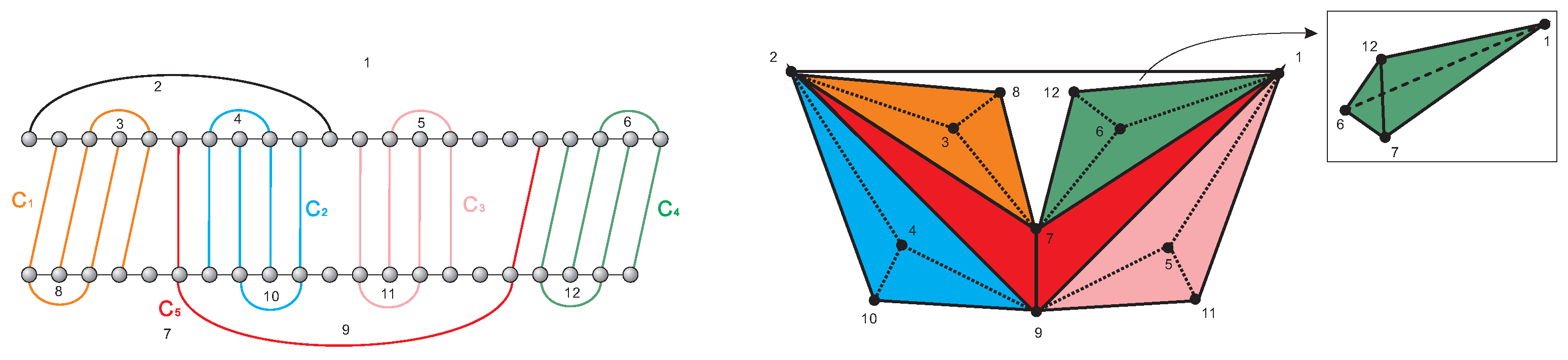
Figure 7 demonstrates a decomposition of into components. In this example, the complex does not a priori contain any free 1-face, whence . It is straightforward to verify that features the five components:
The -arcs of induce the outer block and the inner block . The components are contained in the outer and in the inner block, respectively.
Lemma 3.
Let C be a -component with blocks . Then, for any other component , there exists a unique block, , that contains .
Proof.
Suppose that C--arcs are given by , where and .
Claim: Given a -couple with -arcs and , then there exists a block that contains both and .
Firstly, both endpoints are contained in the same C-block otherwise would cross a C--arc. Suppose and are contained in different C-blocks. Since C and are distinct components, C-couples and -couples are mutually non-crossing. As a result, partitions the C-couples into to two non-empty subsets, one contained in and the other in . By construction, any couple contained in the former subset and any pair in the latter are non-crossing, which is impossible since C is a component.
It follows that there exists a C-block that contains both and .
Any -couple that crosses has at least one -arc contained in . By the above argument, both of its -arcs are then contained in , i.e., contains . Since is a component this implies that any -couple is contained in . □
Lemma 3 gives rise to a relation over the set of -components as follows: if all --arcs are contained in an inner block of . In view of Lemma 3, we can verify that the relation ≺ is a well-defined partial order. In Figure 7, , and are maximal.
We next identify how two 2-simplices that share a mixed edge affect the location of couples along the two backbones. This reflects the planarity of -structures and has important consequences for how components are glued in the loop complex.
Lemma 4.
Let Δ and be -2-simplices that share the mixed edge, ω, and that correspond to the ϕ-arcs and , where . Then any couple where is contained in either
Proof.
Without loss of generality we may assume that features the S-arc . Let , since , by construction and . In case one of the vertices, is contained in and the other is contained in , the arc organizes into distinct S-loops (see Figure 8), which is a contradiction. Thus, are contained in or , i.e., the -arcs associated with are contained in or . □
Lemma 5.
Let C be a -component. Then for any 2-simplex and any 1-face ω, there exists at most one 2-simplex such that .
Proof.
Clearly, the statement holds when is pure. For mixed , by w.l.o.g. let and assume the S-loop corresponds to the arc where .
Suppose there exist distinct 2-simplices having as a 1-face. We shall denote the , and --arcs by , , , respectively. Without loss of generality, we may assume that . Since any -arcs are non-crossing, we have .
We now apply Lemma 4: Since , the couple is contained in or . Since , is contained in .
In view of and belonging to C, there exists a sequence of pairs such that and are crossing.
Lemma 4 applies to any couple , locating it in or . In addition, since and are crossing, is contained in , as is . Analogously, it follows that is contained in , which is, by construction, impossible.
Accordingly, there exists at most one 2-simplex such that . □
Let C be a component and a C-1-face. Lemma 5 implies that is contained in either one or two C-2-simplices. We call a 1-face that is contained in a unique C-2-simplex C-free. Furthermore we call a component C complete if, for any of its 1-faces , there exist exactly two 2-simplices such that and incomplete, otherwise.
Let C be a component with -arcs , where and . Let denote the 2-simplices associated with the -arcs , respectively. Suppose that C--arcs partition the two backbones into the sequence of blocks ordered from left to right and where denotes the outer-block. Let and denote the mixed 1-faces of that are associated with and , respectively. We call the mixed edges and associated with the outer block the C-boundary. Note that and coincide if and only if and share a common mixed edge.
The next lemma constitutes a key observation which facilitates the computation of the homology of -structures via the Mayer–Vietoris sequence, see Theorem 2.
Lemma 6.
Let C be an -component having boundary and , and let be an -component with the property . Suppose that ω is a 1-simplex shared by C and , then or .
Proof.
Let denote the 2-simplices of C associated with the -arcs , ordered from left to right. Suppose that and share a common mixed edge and have the -arcs and , respectively. In view of , is contained in the outer C-block and we may by w.l.o.g. assume that .
The fact , now organizes C relative to in a particular fashion, see Figure 9. Employing Lemma 4 we obtain that, except of , all C-couples partition into the following.
Now we use the fact that that C is a component: Firstly, any -couple and any -couple are by construction non-crossing. Secondly, by construction, is crossing into either only one or , which implies that either one, or , is trivial.
Suppose . Then all C--arcs are contained in which implies . In case , all C--arcs are contained in which implies . Therefore, for the shared 1-edge, , holds or . □
6. The Homology of Components
In order to compute the homology of -structures, we shall first compute the homology of components separately and then integrate this information via the Mayer–Vietoris sequence [18,19]. To this end we adopt a topological perspective of crossing components, taking a closer look at the manifold formed by 2-simplices of a component obtained via gluing along their edges.
Given a component C, two couples if there exists a sequence of pairs such that and share at least one 1-face for . Clearly, is an equivalence relation and partitions all pairs in C into equivalence classes , which we refer to as C-ribbons.
Lemma 7.
The geometric realization of a complete -component, C is a sphere.
Proof.
Suppose that partitions all C-pairs into the ribbons .
Claim 1: The geometric realization of a ribbon, , is a surface without boundary.
Since C is complete, for each 2-simplex and its 1-face , there exists a unique 2-simplex such that . By construction, is further contained in . This implies that the geometric realization of is a compact and connected 2-manifold, i.e., a surface without boundary.
Let denote the -sub-complex consisting of all pure edges for which its loops are T-loops. We shall employ in order to relate the crossing relation with .
Claim 2: is connected, i.e., is a subtree of T.
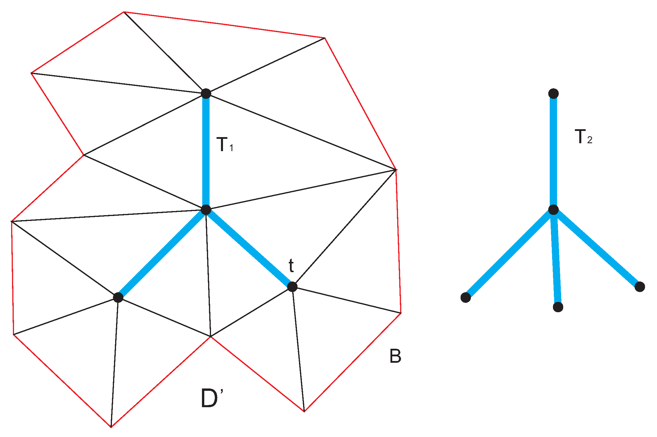
Suppose that contains at least two connected components and . Let denote the subset of 2-simplices of containing at least one -vertex. Since all 2-simplices of are incident to the connected component , the complex formed by is connected. does not contain any -vertices, since otherwise there would, by construction of , exist a pure edge connecting a -vertex and a -vertex, which contradicts the assumption that is disconnected. Thus, is a connected, which is a proper subset of , and its geometric realization is a surface having boundary B, see Figure 10.
The set of 2-simplices containing a fixed -vertex, t, forms a neighborhood of t in the -induced surface, whence any -vertex is contained in the interior of . Consequently, the boundary does not contain any -vertex. From this, we conclude that the boundary, being a cycle, consists of only S-loops. This, however, is impossible since the complex of a secondary structure S is a tree.
Claim 3:C consists of a unique ribbon.
Suppose that C contains at least two ribbons and . Since C is a component, there exists a couple in and not contained in , such that and are crossing.
Without loss of generality, we may consider , , and , see Figure 11. Since and are crossing, the T-loops are on the path connecting T-loops and in the complex of the secondary structure T.
By Claim 2, is connected and thus implies that . Claim 1 guarantees that each 1-face of is not -free, whence there exist two -2-simplices having the face . However, is the unique couple, for which the 2-simplices both contain the pure 1-simplex . As a result the fact that is a surface without boundary guarantees that is contained in , which is a contradiction.
Therefore C is organized as a single ribbon, for which its geometric realization is a surface without boundary. We shall proceed by computing its Euler characteristic .
Suppose that C contains n pairs . Then the complex C features 2-simplices and 1-simplices. Claim 2 stipulates the connectivity of and , whence both and are connected subsets of trees and as such trees themselves. We shall use this in order to count 0-simplices as follows: each pair corresponds to one pure 1-simplex in or . Thus and contain n 1-simplices, which implies that C contains 0-simplices. From this, it follows and C is homeomorphic to a sphere. □
Remark 2.
The key in the proof is to show that the projection of onto each secondary structure, , is connected. If is disconnected, then we can construct a cycle separating different connected components and consisting of only S-loops, resulting in a contradiction. The proof is reminiscent of the Jordan curve theorem in the plane [20,21].
While any complete component is organized as a distinguished ribbon, an incomplete component can consist of multiple ribbons. In Figure 12, the two couples and form an incomplete component, which contains two ribbons and each of which are a couple.
Lemma 8.
Given an incomplete -component C, having the ribbons . Then, for each , there exists some 1-face that is -free.
Proof.
Suppose there exists a ribbon , in which each 1-face is not -free. Lemma 5 guarantees that there exist exactly two 2-simplices such that . Using the argument of Claim 2 of Lemma 7, we can conclude that is connected.
C consists of at least two distinct ribbons since otherwise contains no C-free 1-face, which contradicts the assumption that C is incomplete. Thus there exist a couple and , such that and are crossing. In analogy to Claim 3 of Lemma 7, we can conclude that both and are contained in , which is impossible.
Therefore there exists a 1-face that is -free. □
Theorem 1.
Let C be a component of . Then the following is the case:
and the following is also the case:
where the non-negative integer r depends on C. Furthermore, a complete component, is freely generated by the sum of all C-2-simplices.
Proof.
In case C is complete, by Lemma 7, C is homeomorphic to a sphere, whence and . Clearly, is freely generated by the sum of 2-simplices of C.
In case C is incomplete, suppose that are the C-ribbons. In the following, we prove Equations (1) and (2) by induction on the number k of ribbons.
For , C is a ribbon and, as such, is connected. Since C is incomplete, it contains by Lemma 8 at least one C-free 1-face. This implies that the geometric realization of C is a surface with boundary. Therefore and is free.
For the induction step, we shall combine ribbons in order to compute the homology of an incomplete component. In view of the fact that C is the union of the sub-complexes and , we have the following inclusion maps:
![Mathematics 09 01749 i001]()

Each inclusion map induces a chain map on the corresponding simplicial chain groups and a homomorphism between the corresponding homology groups.
![Mathematics 09 01749 i002]()

Accordingly, we obtain the Mayer–Vietoris sequence
where , and ∂ is the connecting homomorphism given by the zig-zag lemma (see [22,23] for more details).
By Lemma 8, contains at least one -free 1-face, whence its geometric realization of is a surface with boundary. As a result, and is free.
From the definition of ribbon follows, that the intersection of any two ribbons cannot contain any 2-simplices. Furthermore, does not contain any 1-simplices, whence contains only 0-simplices.
In view of , we conclude that consists of only 0-simplices. Therefore, and are free.
In case of , the Mayer–Vietoris sequence reads as follows.
Thus, is an isomorphism.
By induction hypothesis, we have and due to the fact that contains a free -1-face, . Accordingly, we obtain .
In case of , we observe the following:
which gives rise to the following exact sequence.
As a subgroup of the free group , is free and thus projective. As a result, the short exact sequence is split exact and the following:
holds. Since both and are free, we conclude that is free, which completes the proof. □
Theorem 1 shows that, while the complete components contribute only to the second homology, the incomplete components provide generators of the first homology. In terms of discrete Morse theory, each complete component contains a critical point of dimension 2 and each incomplete component can feature multiple critical points of dimension 1.
7. The Main Theorem
In this section, we compute the homology of a -structure. The key tool here is the Mayer–Vietoris sequence, which allows us to connect and compose the homology data of the sub-complexes.
A certain ordering by which the components are glued in combination with Lemma 6 are critical for the application of the Mayer–Vietoris sequence, since they constitute the determinants of how components intersect.
Theorem 2.
Let be the complex obtained from the loop complex of a τ-structure I. Then, is free and the following is the case:
where M denotes the number of complete -components. Furthermore, is freely generated by , where denotes the sum of 2-simplices contained in a complete component, .
Proof.
Let be the -sub-complex induced by the -2-simplices. Suppose that is partitioned into j components . The set and any of its subsets are partially ordered and, by recursively removing maximal components, we can obtain a “descending” sequence such that the following obtains.
This sequence gives rise to a sequence of sub-complexes, obtained by recursively adding a component as follows: and . By construction, we have .
We next prove by induction on the number of components, k, that is free and , where denotes the number of complete components in .
For the induction basis , itself is a component and its homology has been computed in Theorem 1. Clearly, when is complete, is freely generated by the sum of 2-simplices of .
For the induction step we consider as the union of two sub-complexes and and shall combine and by means of the Mayer–Vietoris sequence as follows.
By construction, for any , which enables the application of Lemma 6. We accordingly conclude that the 1-skeleton of is contained in .
In view of , for any i and j, we derive that the 1-skeleton of is contained in . This severely constrains , which consists of 0-simplices and at most two 1-simplices.
As a result, and are free.
In case , we have the following.
Thus, is an isomorphism and . By induction hypothesis, , where denotes the number of complete components in . Due to Theorem 1, in case of being complete and in case of being incomplete. Thus, we can conclude by induction
Clearly, is freely generated by , where is given by the sum of 2-simplices of the -th complete component.
In case , we have the following.
and the following short exact sequence follows.
As a subgroup of the free group , is free and thus projective. Then the short exact sequence is split exact and the following is the case.
Since both and are free, we can conclude that is free.
Therefore it follows by induction that is free and , where M denotes the number of complete components in .
In view of Proposition 9, we have the following:
and is free, which completes the proof. □
The transitive closure with respect to -crossing produces an equivalence relation, i.e., , if there exists a sequence of arcs such as the following:
such that two consecutive arcs and are -crossing for .
An arc-component, A, is an -equivalence class of arcs such that A contains at least two arcs. A is of type 1 if both endpoints of any of its arcs are incident to -arcs and of type 2, otherwise.
Suppose that , where and are -arcs associated with A. These partition the two backbones into blocks: the outer block and the inner blocks , .
Lemma 9.
In , let A be an arc-component of type 1 with blocks . Then, for any arc , there exists a unique block, , that contains i and .
Proof.
Without loss of generality, we may assume that is an S-arc. Since each -arc is incident to at most one arc due to Lemma 1, is not incident to any -arc associated with A and thus its endpoints are contained in A-blocks.
By construction, any T-arc of A, and are non-crossing, since otherwise would belong to the arc-component A. Accordingly, and are either contained in the interval or and we can conclude that A-arcs contained in either or .
Suppose that i and are contained in different blocks, then and are nontrivial. By construction, any -arc and any -arc are non-crossing, which is impossible since A is an arc-component. As a result i and are contained in a single A-block. □
Remark 3.
Lemma 9 is the “arc”-analogue of Lemma 3 for arc-components of type 1. Note that the statement does not hold for arc-components of type 2.
Given an arc-component A of type 1 in the interaction structure , each -arc is associated with exactly one 2-simplex, as Lemma 1 guarantees that each -arc is incident to at most one arc. Let denote the 2-simplices associated with the -arcs , respectively. Let and denote the mixed 1-faces of that are associated with and , respectively.
Lemma 10.
Let A be an -arc-component of type 1 with blocks . Let denote the 2-simplices associated with A and and be the mixed 1-faces of that are associated with and , respectively. Then for and .
Proof.
Let denote the -arcs associated with A ordered from left to right. It suffices to prove . Set , where s and t are S-loops and T-loops associated with . Clearly, and .
By Lemma 9, any -arc is either contained in or its complement. This guarantees that and belong to the same S-loop s and, furthermore, that and belong to the same T-loop t.
As a result the 2-simplex associated with contains as a mixed face, i.e., . □
Now we are in position to prove the Main Theorem.
Proof of the Main Theorem.
The triviality of the third homology group, , follows from Corollary 1. In view of Lemma 1, Proposition 8 and Theorem 2, we have the following:
where M denotes the number of complete -components.
First we observe that any -butterfly removal does not change the crossing status of any two arcs. Thus, there is a natural bijection between the set of I-arc-components and that of -arc-components. Moreover, each I-arc-component of type 1 corresponds to an -arc-component of type 1.
It suffices to show that when passing from the complex to , the number of -arc-components of type 1 equals the number M of complete -components.
Claim: there exists a bijection between the set of -arc-components of type 1 and that of complete components of .
Given an -arc-component of type 1, A, let C denote the set of couples associated with arcs of A. In view of Lemma 10, any 1-simplex that appears as a face in C-couples is shared by at least two 2-simplices. As a result, C does not contain any free 1-simplex and passing from X to , simplicial collapses do not affect C-2-simplices.
Consequently, all C-couples in simply persist when passing to , where C itself becomes a -component. Lemma 10 further guarantees that C does not contain any free 1-face, whence Lemma 8 implies that C is complete.
Accordingly, the Ansatz produces a well-defined mapping between arc-components of type 1 and complete -components.
is, by construction, injective since the mapping constitutes a mere reinterpretation of an arc-component of type 1.
In order to establish surjectivity, let be a complete -component. induces a distinguished, unique set of -arcs, . By construction, any two -arcs satisfy , whence is contained in a nontrivial and distinguished arc-component .
We proceed by proving that is an arc-component of type 1. Suppose , then there exist an arc and such that and are -crossing. Note that is associated to a -couple . Let be the pure edge associated with . We showed in the proof of Lemma 7, that is connected.
Since and are -crossing, the S-loops are vertices of from which follows that both s and are on a path of two S-loops in . Accordingly is contained in . Lemma 7 guarantees that is a sphere, whence there exists a -couple for which is a pure face. As a result we obtain , which is a contradiction from which follows.
By Lemma 2, both endpoints of an -arc are incident to -arcs, whence is an arc-component of type 1 and , whence is surjective and, thus, bijective.
Therefore and .
The Euler characteristic of can be expressed as the alternating sum of ranks of its homology groups, i.e., , whence . Theorem 2 shows that is free, from which we can conclude . □
8. Discussion
In this paper we computed the simplicial homology of -structures. -structures represent a meaningful generalization of bi-structures [7,8] as they allow us to study transitions between sequence–structure pairs where the underlying sequences differ in specific manners. Bi-structures would only facilitate the analysis of such pairs, where the underlying sequences are equal. Intuitively, the free energy of such sequence–structure pairs, which is a quantity that is straightforward to compute, characterizes the probability of finding such a pair of sequences in the course of evolution.
We are currently extending the results of this paper by computing the weighted homology of -structures over a discrete valuation ring, R. This entails the study of weighted complexes in which simplices are endowed with weights [9,24,25]. These weighted complexes feature a new boundary map, , where denotes the free R-module generated by all n-simplices contained in X. is given by the following.
As it is the case for bi-structures [9], the weighted homology plays a crucial role in the Boltzmann sampling of sequence–structure pairs that minimize the free energy of the -structure.
Our approach differs from the purely algebraic proofs for the simplicial loop homology of bi-structures [8]. In the case of bi-structures, the computation for the second homology employs the fact that their first homology group is trivial. This allows us to understand the second homology group via a long exact sequence of relative homology groups. However, for -structures, the first homology is, in general, nontrivial and therefore requires a different approach.
We first reduce the loop complex to the sub-complex via simplicial collapses, retaining the homology of the original space. We then dissect a certain 1-dimensional sub-complex in Proposition 9 and then decompose into components based on the -crossing of couples. This decomposition allows us to identify different generators of the homology, with incomplete and complete components contributing to the first and second homologies, respectively. Finally, we compute the homology of by gluing components in a particular manner. This makes use of the planarity of -structures in Lemma 6 and assures that we encounter particularly simple intersections, when applying the Mayer–Vietoris sequence. It is worth pointing out that in the proof of Theorem 2 the particular ordering in which the components are glued is crucial.
In view of Proposition 9, Theorems 1 and 2, the generators of the first homology of the loop complex originate from the combining of the sub-complex , incomplete components and the gluing of different components. The detailed descriptions of all these generators are a work in progress and here we restrict ourselves to using the Euler characteristic to express the rank of the first homology group. Only complete crossing components contribute to the second homology and their geometric realizations are spheres. We provide a combinatorial characterization of the generators in I in terms of arc-components of type 1.
As for applications of this framework, we currently employ -structures to investigate the evolutionary trajectories of viruses, such as flus and the Coronavirus. Specifically, we compute the loop homology of evolutionary transitions to gain deeper insight into sequence-structure-function relationships of the virus.
Author Contributions
Conceptualization, T.J.X.L. and C.M.R.; Investigation, T.J.X.L. and C.M.R.; Writing—original draft, T.J.X.L. and C.M.R. Both authors have contributed equally to this work. Both authors have read and agreed to the possible publication of the manuscript.
Funding
This research received no external funding.
Institutional Review Board Statement
Not applicable.
Informed Consent Statement
Not applicable.
Data Availability Statement
Not applicable.
Acknowledgments
We gratefully acknowledge the comments and discussions from Andrei Bura, Qijun He and Fenix Huang.
Conflicts of Interest
The authors declare no conflict of interest.
References
- Waterman, M. Secondary Structure of Single-Stranded Nucleic Acids. In Studies on Foundations and Combinatorics, Advances in Mathematics Supplementary Studies; Rota, G.C., Ed.; Academic Press: New York, NY, USA, 1978; Volume 1, pp. 167–212. [Google Scholar]
- Smith, T.F.; Waterman, M.S. RNA secondary structure. Math. Biol. 1978, 42, 31–49. [Google Scholar]
- Zuker, M.; Stiegler, P. Optimal computer folding of large RNA sequences using thermodynamics and auxiliary information. Nucleic Acids Res. 1981, 9, 133–148. [Google Scholar] [CrossRef] [PubMed]
- Eddy, S.R. Non-coding RNA genes and the modern RNA world. Nat. Rev. Genet. 2001, 2, 919–929. [Google Scholar] [CrossRef] [PubMed]
- Breaker, R.R. Riboswitches and the RNA World. Cold Spring Harb. Perspect. Biol. 2012, 4, a003566. [Google Scholar] [CrossRef] [PubMed] [Green Version]
- Huang, F.W.D.; Barrett, C.; Reidys, C.M. The energy-spectrum of bicompatible sequences. arXiv 2021, arXiv:1910.00190v1. [Google Scholar]
- Bura, A.C.; He, Q.; Reidys, C.M. Loop homology of bi-secondary structures. Discret. Math. 2021, 344, 112371. [Google Scholar] [CrossRef]
- Bura, A.C.; He, Q.; Reidys, C.M. Loop Homology of Bi-secondary Structures II. arXiv 2019, arXiv:1909.01222. [Google Scholar]
- Bura, A.; He, Q.; Reidys, C. Weighted Homology of Bi-Structures over Certain Discrete Valuation Rings. Mathematics 2021, 9, 744. [Google Scholar] [CrossRef]
- Waterman, M. Combinatorics of RNA Hairpins and Cloverleaves. Stud. Appl. Math. 1979, 60, 91–98. [Google Scholar] [CrossRef]
- Howell, J.; Smith, T.; Waterman, M. Computation of Generating Functions for Biological Molecules. SIAM J. Appl. Math. 1980, 39, 119–133. [Google Scholar] [CrossRef] [Green Version]
- Schmitt, W.; Waterman, M. Linear trees and RNA secondary structure. Disc. Appl. Math. 1994, 51, 317–323. [Google Scholar] [CrossRef]
- Penner, R.; Waterman, M. Spaces of RNA secondary structures. Adv. Math. 1993, 217, 31–49. [Google Scholar] [CrossRef] [Green Version]
- Forman, R. A user’s guide to discrete Morse theory. Éminaire Lotharingien De Combinatoire 2002, 48, B48c. [Google Scholar]
- Forman, R. Morse Theory for Cell Complexes. Adv. Math. 1998, 134, 90–145. [Google Scholar] [CrossRef] [Green Version]
- Whitehead, J.H.C. Simplicial Spaces, Nuclei and m-Groups. Proc. Lond. Math. Soc. 1939, s2, 243–327. [Google Scholar] [CrossRef]
- Cohen, M.M. A Course in Simple-Homotopy Theory; Graduate Texts in Mathematics; Springer: New York, NY, USA, 1973. [Google Scholar]
- Mayer, W. Über abstrakte Topologie. Mon. Für Math. Und Phys. 1929, 36, 1–42. [Google Scholar] [CrossRef]
- Vietoris, L. Über die Homologiegruppen der Vereinigung zweier Komplexe. Mon. Für Math. Und Phys. 1930, 37, 159–162. [Google Scholar] [CrossRef]
- Jordan, C. Cours D’analyse de l’École Polytechnique; Gauthier-Villars: Paris, France, 1893. [Google Scholar]
- Thomassen, C. The Jordan-Schönflies theorem and the classification of surfaces. Am. Math. Mon. 1992, 99, 116–130. [Google Scholar]
- Fulton, W. Algebraic Topology: A First Course; Graduate Texts in Mathematics; Springer: New York, NY, USA, 1995. [Google Scholar]
- Hatcher, A. Algebraic Topology; Cambridge University Press: Cambridge, UK, 2005. [Google Scholar]
- Dawson, R.J.M. Homology of weighted simplicial complexes. Cah. Topol. Géométrie Différentielle Catégoriques 1990, 31, 229–243. [Google Scholar]
- Ren, S.; Wu, C.; Wu, J. Weighted persistent homology. Rocky Mt. J. Math. 2018, 48, 2661–2687. [Google Scholar] [CrossRef] [Green Version]
Figure 1.
A -structure.

Figure 2.
Any 3-simplex contains a free mixed 1-face. The loops have the covering arcs , , and , respectively. In view of the -arc , the covering arcs form a 3-simplex . If the mixed edges and were not -free, then there would exist two -arcs and , which are crossing.
Figure 2.
Any 3-simplex contains a free mixed 1-face. The loops have the covering arcs , , and , respectively. In view of the -arc , the covering arcs form a 3-simplex . If the mixed edges and were not -free, then there would exist two -arcs and , which are crossing.

Figure 3.
The -butterfly removal. The simplicial collapse of the butterfly corresponds to splicing vertices in the -structure. Here, , , and . The vertex i is split into two consecutive vertices and j is split into two consecutive vertices . The -arc is replaced with two new -arcs and . Depending on the situation, the arcs are connected in a manner such that the loop and the loop do not intersect.

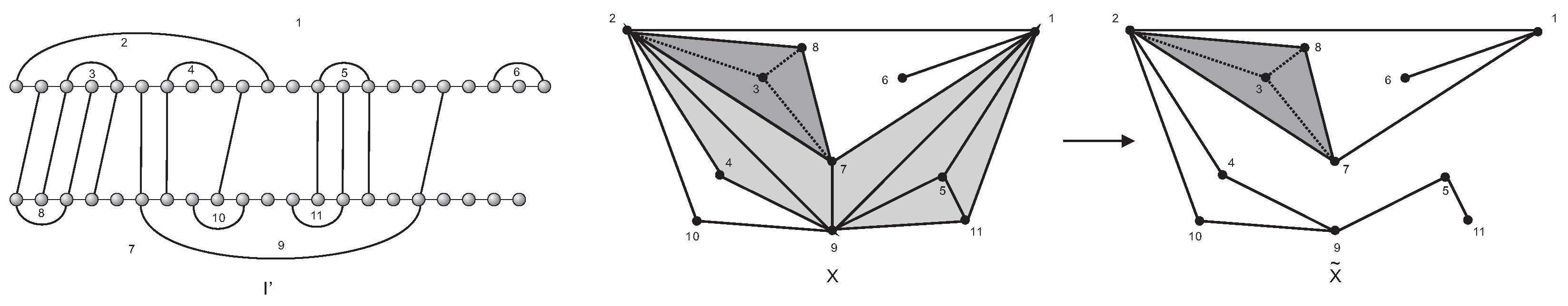
Figure 4.
Simplicial collapse. LHS: A -structure in which each -arc is incident to at most one arc. RHS: X, the complex of and . The underlying sequence of elementary collapses that generates is given by , , , , and . The distinguished empty tetrahedron (darker gray level and dashed lines) cannot be eliminated by simplicial collapses.

Figure 5.
is not unique. Performing the following sequence of elementary collapses on the complex X and is displayed in Figure 4; , , , , and produces a different .
Figure 5.
is not unique. Performing the following sequence of elementary collapses on the complex X and is displayed in Figure 4; , , , , and produces a different .

Figure 6.
Topological stratification. stratifies into a sub-complex induced by all 2-simplices and induced by the remaining 1-simplices.
Figure 6.
Topological stratification. stratifies into a sub-complex induced by all 2-simplices and induced by the remaining 1-simplices.

Figure 7.
Components. LHS: A -structure with labeled loops. RHS: The complex of embedded in the Euclidean space . Note that is identical to . The 2-simplices in are partitioned into five components. The insert (RHS) depicts the component in green, which is an empty tetrahedron.
Figure 7.
Components. LHS: A -structure with labeled loops. RHS: The complex of embedded in the Euclidean space . Note that is identical to . The 2-simplices in are partitioned into five components. The insert (RHS) depicts the component in green, which is an empty tetrahedron.

Figure 8.
The planarity of a -structure. Triangles and share the mixed edge, and correspond to the -arcs and . If an S-arc has its endpoints contained in and , then belong to distinct S-loops, which is a contradiction.
Figure 8.
The planarity of a -structure. Triangles and share the mixed edge, and correspond to the -arcs and . If an S-arc has its endpoints contained in and , then belong to distinct S-loops, which is a contradiction.

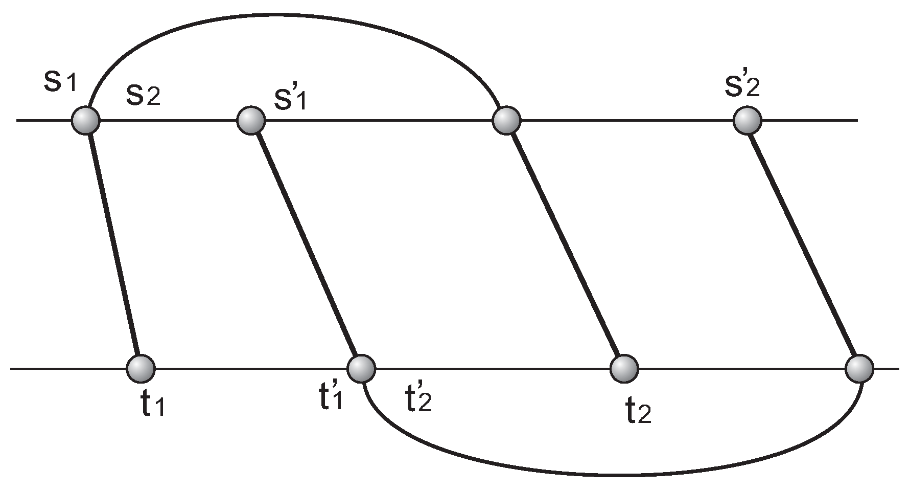
Figure 9.
The fact organizes C-couples into two subsets and , marked by dashed parallelograms.

Figure 10.
The boundary of . The trees and (blue) represent the two connected components of . The sub-complex is formed by 2-simplices of containing at least one -vertex. Then the boundary B of (red) consists of only S-loops.
Figure 10.
The boundary of . The trees and (blue) represent the two connected components of . The sub-complex is formed by 2-simplices of containing at least one -vertex. Then the boundary B of (red) consists of only S-loops.

Figure 11.
A couple and that are crossing, where , , and .

Figure 12.
LHS: A -structure having an incomplete component (colored in blue and with its loops labeled by numbers and its 2-simplices labeled by triangles). RHS: The complex induced by the incomplete component indicates that it contains two ribbons.
Figure 12.
LHS: A -structure having an incomplete component (colored in blue and with its loops labeled by numbers and its 2-simplices labeled by triangles). RHS: The complex induced by the incomplete component indicates that it contains two ribbons.

Publisher’s Note: MDPI stays neutral with regard to jurisdictional claims in published maps and institutional affiliations. |
© 2021 by the authors. Licensee MDPI, Basel, Switzerland. This article is an open access article distributed under the terms and conditions of the Creative Commons Attribution (CC BY) license (https://creativecommons.org/licenses/by/4.0/).
Share and Cite
MDPI and ACS Style
Li, T.J.X.; Reidys, C.M. On the Loop Homology of a Certain Complex of RNA Structures. Mathematics 2021, 9, 1749. https://0-doi-org.brum.beds.ac.uk/10.3390/math9151749
AMA Style
Li TJX, Reidys CM. On the Loop Homology of a Certain Complex of RNA Structures. Mathematics. 2021; 9(15):1749. https://0-doi-org.brum.beds.ac.uk/10.3390/math9151749
Chicago/Turabian StyleLi, Thomas J. X., and Christian M. Reidys. 2021. "On the Loop Homology of a Certain Complex of RNA Structures" Mathematics 9, no. 15: 1749. https://0-doi-org.brum.beds.ac.uk/10.3390/math9151749
Note that from the first issue of 2016, this journal uses article numbers instead of page numbers. See further details here.