Comparing COSTATIS and Generalized Procrustes Analysis with Multi-Way Public Education Expenditure Data

Abstract

Governments serve a variety of purposes, and where governments spend their money has always been of concern to society. In particular, spending on public education is of great interest. However, the volume of this information can be difficult to manage. Therefore, the purpose of this work is to compare the COSTATIS method and generalized Procrustes analysis (GPA) when working with multi-way data. Despite the particular characteristics of each of them, they present similarities and differences that, when analyzed together, can provide complementary results to researchers. The COSTATIS consists of a co-inertia analysis of the compromise of two k-table analyses. The GPA method provides an optimal superimposed representation of individual configurations, and a common consensus configuration is constructed as the mean of all transformed configurations. In addition, the GPA method includes the translation, rotation and scaling of coordinates. In this study, both methods were applied, and the advantages and disadvantages of each are presented. The treated data are a sequence of tables from various countries where different public expenditures on education have been measured over time.

1. Introduction

Education is a fundamental human right for the achievement of stable relations among people, and it is an essential part of the welfare state. Quantifying the efficiency of public expenditure to support education provides the opportunity to accumulate large amounts of data. This is very important because it highlights solutions to improve educational indicators [1]. Researchers typically analyze the efficiency of the public sector in numerous member states, countries and communities. Datasets can be multidimensional as they are collecting information from objects and variables obtained from various periods (three-way data) (I × J × K). It is also interesting to study multiblock data with several hierarchically organized blocks, as there can be partitions due to objects, variables or time. In the treatment of these data, various statistical techniques have been developed that enable a simultaneous analysis of the tables under study by obtaining a consensus structure capable of synthesizing all the available information.

There are numerous techniques that help to interpret three-way data structures. Two methods belonging to different study perspectives for analyzing multiple data tables are the COSTATIS technique of the French Data Analysis school [2] and generalized Procrustes analysis (GPA) of the Anglo-Saxon school [3]. These methods allow the analysis of multiple tables and, as their main objective, both methods aim to search for a common structure (consensus configuration) for the different conditions, differing in the way in which the structure is constructed. The R Project developed Statistical Computing for both methods [4].

The COSTATIS method works with two sets of three-way data to provide a co-structure analysis. In other words, COSTATIS studies the underlying common relationship between data matrices. It consists of a co-inertia analysis of two compromises obtained from two k-table analyses. Thus, it is based on STATIS method (the French expression “Structuration de Tableaux À Trois Indices de la Statistique”), developed by Des Plantes [5] and formalized from a functional analysis point of view by Lavit [6], although the theoretical bases of this method belong to Escoufier [7]. The STATIS method also uses co-inertia analysis developed by Doledec and Chessel [8], which is an extension of the “inter-battery” analysis, considered the first step in partial least squares regression. The COSTATIS method is popular for ecology and environmental information [9,10]. COSTATIS has also been used in fields such as economics [11]. In contrast, GPA is an entirely geometric technique based on the search for an optimal consensus configuration, in the sense of approximating as closely as possible the different configurations associated with each individual-variable matrix.

Through these methods, databases with significant information can be studied in a more complex way. One of the characteristics of these techniques is that they offer graphical representations of the cloud of individuals characterized by the variables of each table and by the set of variables on the same factorial plane, being able to observe the proximities between the individual points of the different tables. The interpretation is intuitive, transferring this facility to the more complex methods. This method has been used in different fields, for example, to analyze sensory profiling data [12] and anatomical marker placement [13] as well as to model growth and age- and sex-related changes in the shape of the pediatric thoracic spine [14] and relationships between experts or panelists [15,16].

The aim of this paper is to provide insight into the ideas of these methods (COSTATIS and GPA). The results will be explored from both points of view and will show how the outputs of the two methods can be used to interpret the relationships between indicators of public spending on education in different countries.

2. Generalized Procrustes Analysis

Procrustes analysis is a multivariate statistical technique that is applied for multiple data blocks. The objective of Procrustes analysis is to match two configurations of N points in K dimensions by translation, rotation/reflection and possibly isotropic scaling. Following Procrustes analysis, generalized Procrustes analysis (GPA) was developed, which simultaneously adjusts to the consensus (or average) configuration, in the Procrustes sense, of L configurations of N points in K. It was introduced by Kristof and Wingersky [17] and popularized by Gower [3].

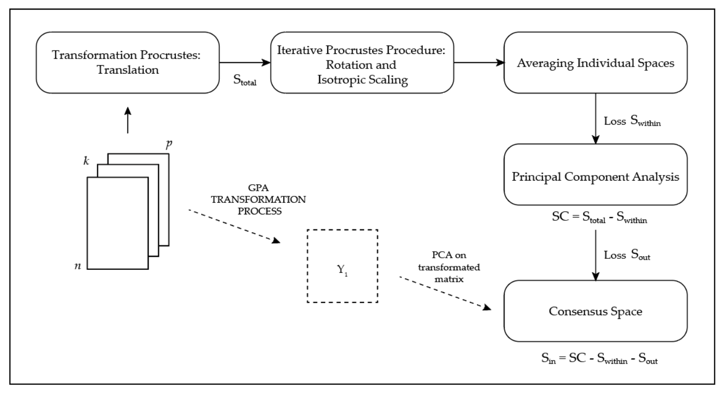
GPA consists of two steps: (A) Procrustes transformation followed by (B) principal component analysis (PCA) on the transformed data blocks (optional). In this algorithm, the points of every object are translated, scaled and rotated iteratively until the least squares fit of all objects to a consensus object is no longer improved.

Mathematically, the transformations applied in Procrustes analysis can be expressed as follows:

$${\mathrm{Y}}_{\mathrm{k}}={\mathsf{\rho }}_{\mathrm{k}}{\mathrm{X}}_{\mathrm{k}}{\mathrm{H}}_{\mathrm{k}}+{\mathrm{T}}_{\mathrm{k}}$$

(1)

where ${\mathrm{Y}}_{\mathrm{k}}$ represents the Procrustes transformation, ${\mathrm{T}}_{\mathrm{k}}$ is the matrix of translation constants, which is easily handled by simply subtracting the mean, and ${\mathrm{H}}_{\mathrm{k}}$ represents the rotation matrix.

After each individual rotation matrix is computed, the new rotated individual matrix (${\mathrm{X}}_{\mathrm{k}}{\mathrm{H}}_{\mathrm{k}}$) and the group average matrix are recomputed for all the k sets. After these computations, ${\mathsf{\rho }}_{\mathrm{k}}$ represents the isotropic scaling factor. A configuration k is shrunk when $0<{\mathsf{\rho }}_{\mathrm{k}}<1$ and stretched when $1<{\mathsf{\rho }}_{\mathrm{k}}$, the iteration method is used.

The translation can be taken care of by column centering of each variable first [3]. The sum of all the squared distances between the individual transformed matrices is the criterion minimized by GPA, which can be written as:

$$\mathrm{K}{\displaystyle \sum }_{\mathrm{k}=1}^{\mathrm{k}}\parallel \mathrm{C}-{\mathsf{\rho }}_{\mathrm{k}}{\mathrm{X}}_{\mathrm{k}}{\mathrm{H}}_{\mathrm{k}}\parallel$$

(2)

Note that ${\mathrm{H}}_{\mathrm{k}}$ is an orthogonal matrix;${ \mathrm{H}}^{\mathrm{T}}\mathrm{H}={\mathrm{HH}}^{\mathrm{T}}=\mathrm{I}$ and on the isotropic scaling factors ${\mathsf{\rho }}_{\mathrm{k}}$:

$${\displaystyle \sum }_{\mathrm{k}=1}^{\mathrm{k}}\parallel {\mathsf{\rho }}_{\mathrm{k}}{\mathrm{X}}_{\mathrm{k}}{\mathrm{H}}_{\mathrm{k}}\parallel =\mathrm{K}$$

(3)

C represents the consensus matrix in all transformed blocks

$$C=\frac{1}{\mathrm{m}}{{\displaystyle \sum }}_{\mathrm{i}=1}^{\mathrm{m}}{\mathsf{\rho }}_{\mathrm{i}}{\mathrm{X}}_{\mathrm{i}}{\mathrm{H}}_{\mathrm{i}}$$

(4)

GPA uses the ANOVA to identify significant effects of the transformations. The total variance can be partitioned as follows:

$${\mathrm{S}}_{\mathrm{total}}={\mathrm{S}}_{\mathrm{in}}+{\mathrm{S}}_{\mathrm{out}}+{\mathrm{S}}_{\mathrm{within}}$$

(5)

in which ${\mathrm{S}}_{\mathrm{total}}$ is the total variance contained in the data where:

$${\mathrm{S}}_{\mathrm{total}}=t\mathrm{r}{{\displaystyle \sum }}_{\mathrm{i}=1}^{\mathrm{m}}\left({\mathsf{\rho }}_{\mathrm{i}}^2{\mathrm{X}}_{\mathrm{i}}{\mathrm{X}}_{\mathrm{i}}^{\prime }\right)$$

(6)

Before the iterative procedure ${\mathrm{S}}_{\mathrm{total}}$ is scaled to remain constant.

The parts ${\mathrm{S}}_{\mathrm{in}}$ and ${\mathrm{S}}_{\mathrm{out}}$ together constitute the consensus variance, where ${\mathrm{S}}_{\mathrm{in}}$ is the part explained by the first Q dimensions of the consensus-space, and ${\mathrm{S}}_{\mathrm{out}}$ is the part left unexplained, this being the part associated with the higher dimensions of the consensus-space. The ${\mathrm{S}}_{\mathrm{within}}$ is the part lost in averaging the obtained individual spaces to the consensus-space and constitutes the Least Squares or Procrustes criterion minimized.

Then, to reduce the dimensionality of C, PCA is often used. It calculates the consensus configuration of the sample and allows the results to be plotted on two-dimensional maps.

The steps of the GPA are clearly reflected in the following diagram (Figure 1).

3. COSTATIS

COSTATIS was introduced by Thioulouse [2]. It is an exploratory method of three-way multivariate data analysis methodology based on two data analysis techniques: co-inertia analysis (COIA) [8,18] and variant of STATIS-like analysis (although the original paper used partial triadic analysis (PTA)) [2,19,20]. The purpose is to analyze the relationships between the structures of two sets of data matrices as a whole. The method consists of two steps:

1.

First, a variant of STATIS-like analyses [19,21] performed to identify the stable structure in a k-table. In this paper, a STATIS has been carried out, allowing the use of public education expenditure in two sets of countries with different economic characteristics. In this case, the method consists in performing two STATIS analyses: one on k-tables of high economic level countries, and another on the k-tables of low economic level countries that measure sets of variables collected on the same observations. The result is the mean table of maximum inertia, which represents the ‘‘compromise’’ and captures the similarities among the k individual tables constituting the k-table.

STATIS method is performed in order to compare and analyze the relationship between the different data sets, to combine them into a common structure called a compromise, which is then analyzed via PCA to reveal the common structure between the public education expenditure, and finally to project each of the original data sets onto the compromise to analyze similarities and differences. PCA performed on the variance–covariance matrix of this composite table provides information on expenditures as a function of the indicators measured during several years.

STATIS is a generalization of PCA. The algorithm is developed as follows:

A.

The first stage consists to compare the structure s of the K matrices to each other and to come up with a so-called inter-structure. This can be summarized as follows:

(1)

Calculate the K variance–covariance matrices as:

$${\mathrm{W}}_t={\mathrm{X}}_{\mathrm{t}}{\mathrm{Q}}_{\mathrm{t}}{\mathrm{X}}_{\mathrm{t}}^{\ast }$$

(7)

where for each data table the variance-covariance matrix ${\mathrm{W}}_t$ (I × J) reflecting the similarities between I objects within this data table. ${\mathrm{X}}_{{\mathrm{t}}_{\mathrm{i}}}$ is a matrix of dimension I × J_t and all ${\mathrm{X}}_{\mathrm{t}}$ matrices of X have the same number of variables; ${ \mathrm{X}}_{\mathrm{t}}^{\ast }$ is the transposed matrix of ${\mathrm{X}}_{\mathrm{t}}$ and ${\mathrm{Q}}_{{\mathrm{t}}_i}$ is the identity matrix of dimension J × J. In this study, all matrices had the same number of attributes, J_i = J for each k, and the same weight was given to all the individuals/simples.

Each matrix ${\mathrm{X}}_k$ defines implicitly a structure for the individuals, which depends on their respective positions as defined by the distances between each pair of individuals:

(2)

Calculate the matrix of RV coefficient:

$$RV\left(W_k,W_{k^{\prime }}\right)=\frac{Tr\left(W_{k}D{W}_{k^{\prime }}D\right)}{\sqrt{Tr{\left(W_{k}D\right)}^2{\left(W_{k^{\prime }}D\right)}^2}}$$

(8)

The RV coefficients are non-negative and ranges from 0 to 1.

(3)

Perform PCA of the RV matrix $\left[\mathbf{S},\mathbf{V},\mathbf{S}\right] =\mathrm{SVD}\left(\mathbf{R}\mathbf{V}\right)$, SVD is the singular value decomposition version of PCA.

$${\mathrm{a}}_{\mathrm{k}}=\raisebox{1ex}{$S_1$}\!\left/ \!\raisebox{-1ex}{$\sum \mathrm{k}$}\right.=1K{S}_1$$

(9)

$S_1$ (K × 1) is the first column vector of the matrix S

B.

The second step of the method is the determination of the intra-structure, that is, the search for a common structure to the structures corresponding to the K instants.

(1)

Calculate the compromise among tables as:

$$W=\sum \mathrm{k}=1K_{{\mathrm{a}}_{\mathrm{k}}}{W}_{\mathrm{k}}$$

(10)

(2)

Perform PCA of W:

$$\left[\mathbf{L},\mathbf{V},\mathbf{L}\right] =\mathrm{SVD}\left(\mathbf{W}\right)$$

(11)

(3)

Display the compromise score plot.

C.

The third step of the method is the development of the observations’ trajectories. The trajectories show which individuals or observations account for the distances observed among the objects ${\mathbf{W}}_{\mathrm{k}}$ in the inter-structure step.

2.

The second stage is a co-inertia analysis, which is performed on analysis of the compromises of these two STATIS (or variants) to describe the co-structure between the stable part of high economic level countries data and the stable part of low economic level countries data. The COIA summarizes as well as possible the squared covariances between public expenditure on education in the two sets of countries [2].

4. GPA versus COSTATIS

COSTATIS method is a handy tool for studying co-structures of multiple data matrices. It captures the variation between two consensus structures showing k-tables information, maximizing the variance. It is very flexible and easy to interpret due in some ways to its use of COIA [22].

The co-inertia between two data matrices, X and Y, is the sum of squared covariances:

$${\mathrm{CoIner}}_{\mathrm{XY}}=\mathrm{traza}\left(X{D}_{J\ast }{X}^T{D}_{I}Y{D}_{J\ast \ast }{Y}^T{D}_I\right)$$

(12)

where $X^T{D}_{I}X{D}_{J\ast }$ and $Y^T{D}_{I}X{D}_{J\ast \ast }$ are the spectral decomposition of generalized PCA. $X^T$ and $Y^T$ are the transposes of the matrices X and Y. $D_{J\ast }$ and $D_{J\ast \ast }$ are two hyperspace matrices of the first and second matrix, respectively. Additionally, $D_I$ is the diagonal of matrix (I × I) of matrices’ rows weights, where $D_I =Diag(w_1,\dots ,w_I)$.

That is, COIA maximizes the square covariance between two sets, in this case of public education expenditures in high- and low-income countries. Additionally, results can be represented graphically by drawing arrows, where the origin point signifies information of the first data set and the tip of arrow the second data set. A shorter arrow better explains the structure found in the matrices.

Besides, COSTATIS method reflects the structure of those matrices highly correlated with the first eigenvector of the vector correlation matrix of the respective STATIS analyses, so it will highlight similar structures where the first common principal direction coincides. It has the advantage of preserving the optimality properties of the compromises of the two STATIS analysis; therefore, it looks for the relationships between two stable structures. COSTATIS should be preferred when the two data sets’ relationships are strong, and chronological structures are not of primary importance.

This method allows plotting both the compromise of two study sets and the final COIA results. The example presented in this article is based on two public expenditures on education datasets from 2005 to 2019: one in p high-income countries and another in q low-income countries. The execution of COSTATIS method presents the countries’ compromises: one for the high economic level and one for the low economic level, and it draws the COIA of these two compromises (see Figure 2).

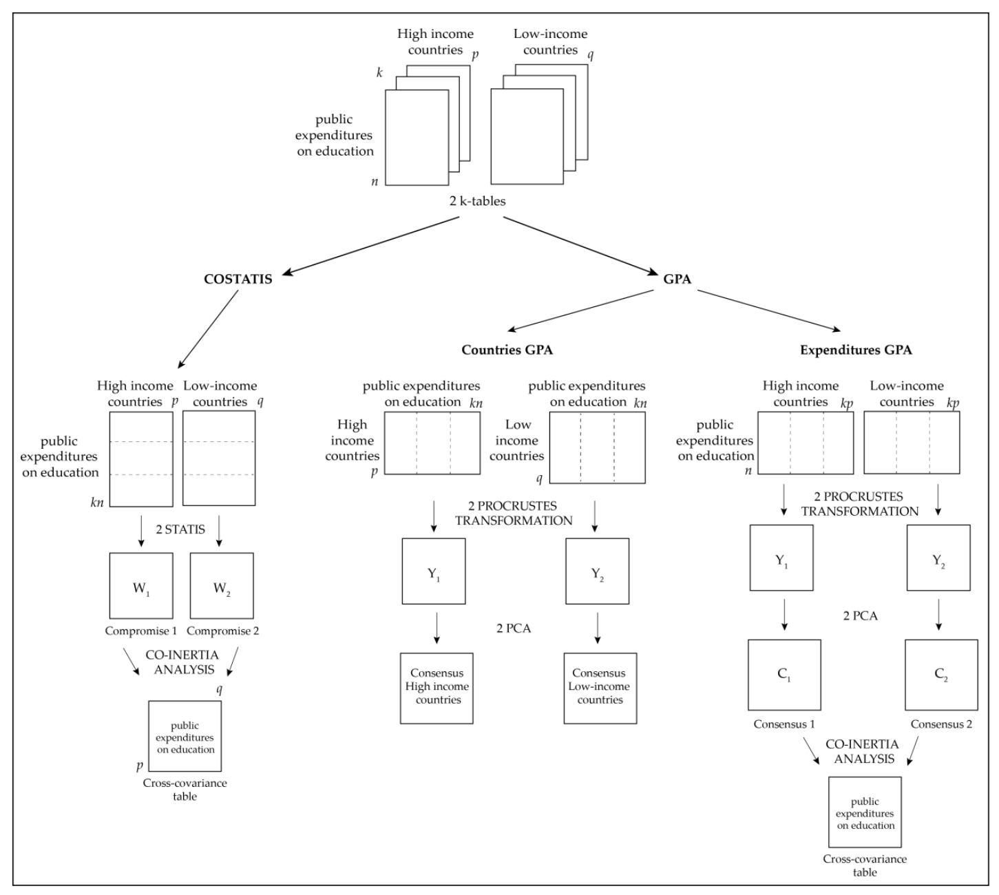
GPA method can provide an optimal overlapping representation of the individual configurations, generating a common consensus configuration as the average of all transformed configurations of original matrices to be analyzed. However, this analysis is intended for a single set of tables, not for two. Therefore, it is not possible to compare this technique with COSTATIS method directly. For comparison, the same two datasets are used as a starting point (two public expenditures on education datasets from 2005 to 2019, in p high-income countries and q low-income countries), GPA will be applied in two different ways: one in order to represent the consensuses of p and q countries and the other for the consensuses of n expenditure variables with which to perform a COIA that allows the co-inertia of structures to be plotted. Figure 2 schematically illustrates the procedure for the application of the methods to be carried out.

COSTATIS and GPA share the same restrictions on rows and columns of matrices, which must always be identical in each set: same rows and same columns for all times, i.e., same public education expenditure variables and same countries for years 2005 to 2019. In COSTATIS, the two sets of tables may have different numbers of columns (countries), while rows (public education expenditure variables) must be the same for all tables at all times (years). In GPA to represent consensus of the two groups of countries (Countries GPA), each set of tables has same number of countries (in rows) and public education expenditure variables (in columns) for all tables at all times (years). Additionally, in GPA to represent the co-structure of public education expenditures of the two groups of countries (Expenditures GAP), each set of tables has the same number of expenditure variables (in rows) and countries (in columns) for all tables at all times (years).

5. Case Study

5.1. Data

The dataset used in this article is from UNESCO Institute for Statistics (UIS) statistical database (http://data.un.org/, accessed on 1 May 2020). The data are a sequence of tables from various European countries where different public expenditures on education have been measured over time (from 2005 to 2019). We worked with the average expenditure for three time periods: from 2005 to 2009, from 2010 to 2014 and from 2015 to 2019.

Table 1. List of the codes of public expenditures on education.

Code	Type of Expenditure
SCE	All staff compensation as % of total expenditure in public institutions (%)
CEP	Capital expenditure as % of total expenditure in public institutions (%)
CES	Current expenditure other than staff compensation as % of total expenditure in public institutions (%)
LPRE	Expenditure by level of education: pre-primary (as % of government expenditure)
LPRI	Expenditure by level of education: primary (as % of government expenditure)
LSEC	Expenditure by level of education: secondary (as % of government expenditure)
LTER	Expenditure by level of education: tertiary (as % of government expenditure)
GEE	Government expenditure on education (% of government expenditure)
PEE	Public expenditure on education (% of GDP)

presents the types of expenditure analyzed together with the codes assigned.

The European countries to be studied were: Austria, Cyprus, Czechia, Finland, Hungary, Iceland, Ireland, Italy, Lithuania, Norway, Poland, Portugal, Romania, Slovakia, Slovenia, Spain, Sweden, Switzerland and the United Kingdom. These were divided into two groups according to the economic level indicated by the International Monetary Fund; taking into account nominal GDP in millions of US dollars (USD) [23].

• Group 1 consists of countries with a nominal GDP above USD 300 million: Austria, Ireland, Italy, Norway, Poland, Spain, Sweden, Switzerland and the United Kingdom.
• Additionally, group 2 consists of countries with a nominal GDP of less than USD 300 million: Cyprus, Czechia, Finland, Hungary, Iceland, Lithuania, Portugal, Romania, Slovakia and Slovenia.

5.2. Procedure

COSTATIS method was used to show the relationship between public education expenditure structures in countries with high economic status and countries with low nominal GDP, from 2005 to 2019. Therefore, data were organized in two tables with 27 rows each, containing data for the 9 public expenditures variables on education during the 3 time periods indicated above. One table has 9 columns, which contains data for the group of countries with a high nominal GDP (above USD 300 million), and another table has 10 columns, which contains data for the group of countries with a low nominal GDP (below USD 300 million).

In the first application of GPA method, data were organized to examine the structures of public expenditure on education in countries with high nominal GDP and countries with low nominal GDP. In this case, a table contains 9 rows corresponding to countries with high economic status and 27 columns with information on different expenditures over time (9 public expenditures variables on education × 3 time periods). Additionally, another table contains 10 rows corresponding to countries with a low economic status and 27 columns with information on education expenditures over time. In the second application of GPA method, data were organized in order to find out the relationship between both structures of public expenditure on education in both groups of countries (with high and low nominal GDP). The information was processed in two tables with 9 rows each, corresponding to the different public expenditures on education. One table had 27 columns (9 countries with high nominal GDP × 3 time periods) and the other had 30 columns (10 countries with low nominal GDP × 3 time periods). This technique, applied to both tables, provides the consensus matrix for each group of countries. Additionally, a co-inertia analysis was performed on these consensus matrices.

Both from the point of view of the COSTATIS method and from the point of view of the GPA, the objective was to investigate the co-structure between two data tables by summarizing as best as possible the squared covariances between high and low economic countries.

Analyses were carried out with R Program 3.5.3. for statistical computing [4] (package ‘ade4’ version 1.7-15 [24] and package ‘FactoMineR’ version 2.4 [25]).

6. COSTATIS Results

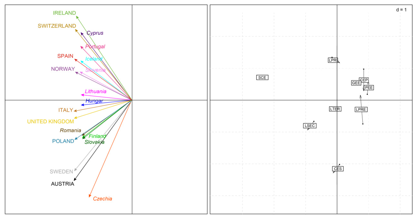
In order to analyze public expenditure on education from 2005 to 2019, in several European counties with high and low economic status, COSTATIS method was carried out. This method presents a first axis with 80.23% of explained inertia. RV coefficient is acceptable (0.979), indicating correlation between the structures. The representation of compromise matrices (obtained from the two STATIS) in factor planes makes it possible to characterize the common structures, in terms of public expenditure on education, during the stability and/or instability detected from 2005 to 2019 (see left side of Figure 3). Countries analyzed are distributed along the ordinate axis. The structure of the highest economic level countries shows four countries at the top of the factorial plane (Ireland–Switzerland and Spain–Norway), and five at the bottom (Italy–UK–Poland and Sweden–Austria). Ireland, Switzerland, Sweden and Austria show greater stability as longer arrow lengths are observed. The structure of the lowest economic level countries shows four countries at the top of the factorial plane (Cyprus, Portugal, Iceland and Slovenia), two in the middle (Lithuania and Hungary), and four at the bottom (Romania, Finland, Slovakia and Czechia). Czechia shows great stability. The cross-tabulation shows the highest values between Spain and Portugal (0.992), Cyprus and Switzerland (0.993), and Slovenia with Italy (0.996), Spain (0.996) and UK (0.990). Additionally, the lowest values between Czechia with the nine high economic level countries and Ireland with Finland, Romania and Slovakia.

Co-inertia analysis graph illustrates the strength of relationship between the structure of high- and low-income countries, in terms of public expenditure on education from 2005 to 2019 (see right side of Figure 3). Each expenditure variable is represented by two dots joined by an arrow. The origin of the arrow corresponds to the structure of countries with high nominal GDP and the end of the arrow corresponds to the structure of countries with low nominal GDP. The length of these arrows is thus a measure of the discrepancy between the two data tables. The strong cross-covariances between the country data in the two tables mean that the variables are similar. Therefore, the short arrows indicate a strong underlying relationship between two structures, i.e., expenditure variables behave similarly in high and low economic countries. Of particular note in this respect are remuneration of all staff (SCE), expenditure at the tertiary level of education (LTER) and public expenditure on education as a share of total public expenditure (GEE). For example, the weight of public employees’ salaries in public institutions in terms of education in the Spanish economy was at levels similar to those of other developed countries [26]. The larger the arrows, the more significant the discrepancies between the two countries groups. Here, capital expenditure (CEP) and expenditure at the pre-primary level of education (LPRE) stand out. In addition, a pattern is observed between capital expenditure (CEP), total public expenditure (GEE) and public expenditure on education in terms of GDP (PEE). On the left hand side, the projection of public expenditures on education in the factor map of the COSTATIS analysis shows that remuneration of all staff (SCE) is a very relevant expenditure in Norway and Slovenia. Expenditure at the secondary education level (LSEC) characterizes countries such as Poland, Sweden, Austria, Romania, Finland and Slovakia. However, the other public expenditures do not determine the countries analyzed as much.

7. GPA Results

For the same purpose of analyzing public expenditure on education from 2005 to 2019, in several European countries of high and low economic level, GPA was used. The results of GPA method show a high similarity between the matrices for the three time periods (2005–2009, 2010–2014 and 2015–2019). For each group of countries (high and low economic level), countries GPA presents RV coefficients close to unity (group 1: 0.660, 0.753 and 0.715; group 2: 0.871, 0.718 and 0.799). Additionally, expenditures GPA presents RV coefficients very close to unity (group 1: 0.999, 0.990 and 0.989; group 2: 0.996, 0.987 and 0.992). The results are plotted on two axes for comparison with those obtained with COSTATIS method. The left-hand side of Figure 4 represents consensus configuration of both countries’ groups with their trajectories on the foreground factorial plane. In countries with a nominal GDP above USD 300 million: Spain and the United Kingdom are very close to each other indicating high similarity. Italy and Switzerland are near to these, although to a lesser extent. Additionally, Norway, Poland and Sweden are also similar to each other. In countries with a nominal GDP less USD 300 million: Portugal and Cyprus are close to each other indicating similarity. The same is true for Finland, Slovakia and Romania. The trajectories (of the 3 time periods) are irregular. Czechia, Poland, Romania and Iceland stand out for their considerable dispersion, i.e., large discrepancies between 2005–2009, 2010–2014 and 2015–2019.

The difference between the configurations can be analyzed with the contribution of each type of expenditure to the residual sum of squares in the ANOVA associated with the GPA (PANOVA), these results are presented in

Table 2. Procrustes analysis of variance (PANOVA).

Countries with High Nominal GDP				Countries with Low Nominal GDP
Group 1	Sum of squares within by country			Group 2	Sum of squares within by country
	SSfit	Ssresidual	SStotal		SSfit	Ssresidual	SStotal
Austria	13.695	0.502	14.197	Cyprus	14.885	0.265	15.151
Ireland	14.074	0.850	14.924	Czechia	23.805	2.284	26.089
Italy	9.400	1.023	10.422	Finland	7.219	0.445	7.665
Norway	8.622	0.407	9.030	Hungary	2.204	0.995	3.198
Poland	10.764	1.617	12.381	Iceland	7.915	1.142	9.057
Spain	5.528	0.555	6.082	Lithuania	3.673	0.557	4.230
Sweden	12.597	0.836	13.434	Portugal	19.597	0.430	20.026
Switzerland	7.325	0.661	7.986	Romania	4.545	1.456	6.001
United Kingdom	8.304	3.240	11.544	Slovakia	5.240	1.305	6.545
				Slovenia	1.384	0.654	2.038
sum	90.309	9.691	100.000	sum	90.467	9.533	100.000
Expenditure	Sum of squares within by type of expenditure			Expenditure	Sum of squares within by type of expenditure
	SSfit	Ssresidual	SStotal		SSfit	Ssresidual	SStotal
SCE	61.997	0.039	62.036	SCE	58.188	0.012	58.200
CEP	7.700	0.021	7.722	CEP	7.319	0.021	7.340
CES	0.786	0.056	0.842	CES	3.268	0.202	3.470
LPRE	7.653	0.071	7.724	LPRE	5.799	0.035	5.834
LPRI	0.934	0.024	0.958	LPRI	1.131	0.019	1.150
LSEC	6.423	0.155	6.577	LSEC	9.362	0.198	9.560
LTER	0.400	0.027	0.427	LTER	0.439	0.067	0.506
GEE	3.882	0.026	3.908	GEE	3.990	0.027	4.018
PEE	9.792	0.014	9.806	PEE	9.911	0.013	9.923
sum	99.568	0.432	100.000	sum	99.407	0.593	100.000

. Austria, Ireland and Sweden have the highest sum of consensus and total squares in countries with a high economic level. The same is true for Cyprus, Czechia and Portugal in countries with a lower economic level. The largest discrepancies are observed in Italy, Poland, United Kingdom, Czechia, Iceland, Romania and Slovakia, which have the highest residual sum of squares values. In contrast, Norway, Austria, Spain, Cyprus, Portugal and Finland do not show important differences. On the expenditure side, remuneration of all staff (SCE) stands out in comparison with the rest of the expenditure, with the highest sum of consensus and total squares in both groups of countries. The largest differences are observed for expenditures at the secondary level of education (LSEC), as they have the highest residual sum of squares values. Additionally, in the first group of countries, discrepancies are observed in current expenditures (CES) and expenditures at the pre-primary level of education (LPRE). Public expenditure on education in terms of GDP (PEE) does not differ significantly in high income countries, and SCE, LPRI and PEE expenditure in low-income countries.

Co-inertia analysis graph shows the strength of relationship between the structure of public expenditure on education in both groups of countries (see right side of Figure 4). RV coefficient is 0.987, indicating correlation between the consensus structures. The remuneration variables of all staff (SCE), expenditure by level of education (LPRI, LSEC and LTER) and public expenditure on education as a share of total public expenditure (GEE) behave similarly (short arrows) in high- and low-economy countries. However, less agreement is observed for capital expenditure (CEP) and expenditure at the pre-primary level of education (LPRE).

8. Discussion and Conclusions

COSTATIS and GPA methods analyze the relationship between public education expenditure structures of high- and low-nominal GDP countries from 2005 to 2019. Both methods indicate that remuneration of all staff (SCE), expenditure on the tertiary level of education (LTER), and public expenditure on education as a share of total public expenditure (GEE) behave similarly in both high- and low-economy countries (short arrows in Figure 3 right and Figure 4 right). The expenditures where most differences are observed between high- and low-economy countries are capital expenditure (CEP) and expenditures at the pre-school level (LPRE) (long arrows in Figure 3 right and Figure 4 right). Additionally, there is a pattern between capital expenditure (CEP), total public expenditure (GEE) and public expenditure on education in terms of GDP (PEE), it is not surprising that the public money that each country has is related to capital expenditure and may affect public expenditure on education [1,27,28]. GPA results also report expenditures on primary and secondary education (LPRI and LSEC) that are similar in both groups of countries. These results are in line with those of Halásková and Halásková [27], who indicate the highest percentage of total public expenditures on education in the EU is observed in primary and secondary education, in aggregate accounting for approximately 3.4%.

The compromise results obtained through COSTATIS method coincide with the consensus results obtained through GPA method in that, among high-income countries, Poland and Sweden are very similar in terms of public expenditure on education from 2005 to 2019. Among low-income countries, Portugal and Cyprus are also very similar, as are Finland, Slovakia and Romania. Spain and the United Kingdom stand out for their similarity. COSTATIS method shows, in addition, associations between Spain and Portugal, Cyprus and Switzerland, and Slovenia with Italy, Spain and the United Kingdom. The results are in agreement with those found by Molina, Amate and Guarnido [29] in previous years, and they differ with the research of Halásková and Halásková [27]. However, GPA method provides trajectories for the three time periods, Czechia, Poland, Romania and Iceland show the largest discrepancies between the different years.

By COSTATIS method, it was found that remuneration of all staff (SCE) is a very relevant expenditure in Norway and Slovenia, and expenditure on secondary education (LSEC) characterizes countries such as Poland, Sweden, Austria, Romania, Finland and Slovakia (country projection on co-inertia). In Spain, Neira, Guisán and Rodríguez confirm the consideration of human capital is an essential productive factor for the economic development of a country [30].

Such techniques seek a common or representative structure (compromise or consensus matrix) of matrices for each period of time and their relationship with each other. In many instances, economic studies carry out longitudinal studies to analyze the evolution of objects over time.

Several studies have used COSTATIS method in the context of economics, public expenditures, etc. [11,30,31,32,33]. However, GPA method is the first time it has been used in this context. Moreover, to our knowledge, this is the first study in which a comparative analysis of the two techniques has been carried out.

The two methods presented here reveal important features in the datasets and their analytical relevance. COSTATIS is an eigendecomposition technique that considers the whole space; however, the GPA requires multiple iterations to reach a consensus and to guarantee to converge and considers the specific dimensions, restricted to a subset of these dimensions. As this paper has shown, the two different approaches allow relevant conclusions to be drawn. Both have different advantages and disadvantages, but although at first sight the conclusions obtained seem to be different, they are fully related to the objective of the study and could be used together and depending on the characteristics of the data. From both methods, we can conclude that the behavior of variables remuneration of all staff, expenditure on the tertiary level of education and public expenditure on education as a share of total public expenditure are similarly in both high- and low-economy countries; however, capital expenditure and expenditures at the pre-school level are different in countries taking into account the nominal GDP.

References

- Dutu, R.; Sicari, P. Public Spending Efficiency in the OECD: Benchmarking health care, education and general administration. OECD Econ. Dep. Work. Pap. 2016. [Google Scholar] [CrossRef]
- Thioulouse, J. Simultaneous analysis of a sequence of paired ecological tables: A comparison of several methods. Ann. Appl. Stat. 2011, 5, 2300–2325. [Google Scholar] [CrossRef] [Green Version]
- Gower, J.C. Generalized procrustes analysis. Psychometrika 1975, 40, 33–51. [Google Scholar] [CrossRef]
- R Core Team. R: A Language and Environment for Statistical Computing; R Foundation for Statistical Computing: Vienna, Austria, 2019. [Google Scholar]
- Des Plantes, L. Structuration des Tableaux à Trois Indices de la Statistique: Théorie et Application d’une Méthode D’analyse Conjointe; University of Montpellier: Montpellier, France, 1976. [Google Scholar]
- Lavit, C. Analyse Conjointe de Tableaux Quantitatifs; Masson: Paris, France, 1988. [Google Scholar]
- Escoufier, Y. Le traitement des variables vectorielles. Biometrics 1973, 29, 751–760. [Google Scholar] [CrossRef]
- Doléc, S.; Chessel, D. Co-inertia analysis: An alternative method for studying species—Environment relationships. Freshw. Biol. 1994, 31, 277–294. [Google Scholar] [CrossRef]
- Slimani, N.; Guilbert, E.; El Ayni, F.; Jrad, A.; Boumaiza, M.; Thioulouse, J. The use of STATICO and COSTATIS, two exploratory three-ways analysis methods: An application to the ecology of aquatic heteroptera in the Medjerda watershed (Tunisia). Environ. Ecol. Stat. 2017, 24, 269–295. [Google Scholar] [CrossRef]
- Ladhar, C.; Tastard, E.; Casse, N.; Denis, F.; Ayadi, H. Strong and stable environmental structuring of the zooplankton communities in interconnected salt ponds. Hydrobiologia 2015, 743, 1–13. [Google Scholar] [CrossRef]
- Santos, A.D.; da Silva, N.T.; Castela, G. A COSTATIS approach to business sustainability in turbulent environments from 2008 to 2014. Int. J. Qual. Res. 2019, 13, 887–900. [Google Scholar] [CrossRef]
- Meyners, M. Methods to analyse sensory profiling data—A comparison. Food Qual. Prefer. 2003, 14, 507–514. [Google Scholar] [CrossRef] [Green Version]
- Osis, S.T.; Hettinga, B.A.; Macdonald, S.L.; Ferber, R. A novel method to evaluate error in anatomical marker placement using a modified generalized Procrustes analysis. Comput. Methods Biomech. Biomed. Eng. 2015, 18, 1108–1116. [Google Scholar] [CrossRef]
- Peters, J.R.; Campbell, R.M.; Balasubramanian, S. Characterization of the age-dependent shape of the pediatric thoracic spine and vertebrae using generalized procrustes analysis. J. Biomech. 2017, 63, 32–40. [Google Scholar] [CrossRef]
- Morand, E.; Pagès, J. Procrustes multiple factor analysis to analyse the overall perception of food products. Food Qual. Prefer. 2006, 17, 36–42. [Google Scholar] [CrossRef]
- Zuliani, P.; Bramardi, S.J.; Lavalle, A.; Defacio, R. Caracterización de poblaciones nativas de maíz mediante análisis de procrustes generalizado y análisis factorial múltiple. Rev. Fac. Cienc. Agrar. 2012, 44, 49–64. [Google Scholar]
- Kristof, W.; Wingersky, B. A generalization of the orthogonal Procrustes rotation procedure to more than two matrices. Proc. Ann. Conv. Am. Psychol. Assoc. 1971, 6, 89–90. [Google Scholar]
- Dray, S.; Chessel, D.; Thioulouse, J. Co-intertia and the linking of ecological data tables. Ecology 2003, 84, 3078–3089. [Google Scholar] [CrossRef] [Green Version]
- Thioulouse, J.; Chessel, D. Les analyses multitableaux en écologie factorielle. I. De la typologie d’état à la typologie de fonctionnement par l’analyse triadique. Acta Oecologica Oecologia Gen. 1987, 8, 463–480. [Google Scholar]
- Kroonenberg, P.M. The analysis of multiple tables in factorial ecology: III. Three- mode principal component analysis: “Analyse triadique complete. Acta Oecologica Oecologia Gen. 1989, 10, 245–256. [Google Scholar]
- Jaffrenou, P.A. Sur l’analyse des familles finies de variables vectorielles. In Bases Algébriques et Application à la Description Statistique; Université Claude Bernard: Lyon, France, 1978. [Google Scholar]
- Thioulouse, J.; Simier, M.; Chesse, D. Simultaneous Analysis of a Sequence of Paired Ecological Tables. Ecology 2004, 85, 272–283. [Google Scholar] [CrossRef]
- IMF World Economic Outlook Databases. Available online: https://www.imf.org/en/Publications/SPROLLs/world-economic-outlook-databases#sort=%40imfdatedescending (accessed on 25 June 2019).
- Dray, S.; Dufour, A.B. The ade4 package: Implementing the duality diagram for ecologists. J. Stat. Softw. 2007, 22, 1–20. [Google Scholar] [CrossRef] [Green Version]
- Husson, F.; Josse, J.; Le, S.; Maintainer, J.M. Package “FactoMineR” Title Multivariate Exploratory Data Analysis and Data Mining; R Foundation for Statistical Computing: Vienna, Austria, 2020. [Google Scholar]
- Francisco Varela, A. Business Insider España. 2020. Available online: https://www.businessinsider.es/gasto-salarios-publicos-espana-comparativa-otros-paises-europa-845113 (accessed on 1 May 2020).
- Halásková, M.; Halásková, R. Public expenditures in areas of public sector: Analysis and evaluation in eu countries. Sci. Pap. Univ. Pardubice Ser. D Fac. Econ. Adm. 2017, 24, 39–50. [Google Scholar]
- Castro Fernández, F.D.; González Mínguez, J.M. La composición del gasto público en Europa y el crecimiento a largo plazo. Bol. Econ. 2008, 1, 89–102. [Google Scholar]
- Morales, M.; Fortes, I.A.; Rueda, A.G. El gasto público en educación en los países de la OCDE: Condicionantes económicos e institucionales. eXtoikos 2011, 4, 37–45. [Google Scholar]
- Neira, I.; Guisán, M.C.; Rodríguez, X.A. Análisis cuantitativo del gasto en educación en Europa. In Economic Development; Faculty of Economics and Business: Amsterdam, The Netherlands, 1992. [Google Scholar]
- Delgado, J.P. The Evolution of the Oecd Countries after the 2008 Financial Crisis; Universidade Nova de Lisboa: Lisbon, Portugal, 2019. [Google Scholar]
- Rodríguez-Rosa, M.; Gallego-Ávarez, I.; Galindo-Villardón, M.P.V.-G.M.P. Are Social, Economic and Environmental Well-Being Equally Important in all Countries Around the World? A Study by Income Levels. Soc. Indic. Res. 2017, 131, 543–565. [Google Scholar] [CrossRef]
- Egido, J.; Galindo, P. Dynamic Biplot: Evolution of the Economic Freedom in the European Union. Br. J. Appl. Sci. Technol. 2015, 11, 1–13. [Google Scholar] [CrossRef]
Figure 1.
GPA’s diagram.
Figure 2.
Presentation of the COSTATIS (left) and GPA (right) methods.
Figure 3.
Graphs resulting from COSTATIS method: Euclidean representation of high and low-income countries’ compromises (left) and co-inertia analysis graph of the two compromises (right). The scale is given by the value d.
Figure 4.
Graphs resulting from GPA method: Representation of high and low-income countries’ compromises and their trajectories (left) and co-inertia analysis graph of the two expenditure compromises (right). The scale is given by the value d.