
Models of Strategic Decision-Making under Informational Control

V.A. Trapeznikov Institute of Control Sciences, 117997 Moscow, Russia
Mathematics 2021, 9(16), 1889; https://0-doi-org.brum.beds.ac.uk/10.3390/math9161889
Submission received: 3 July 2021
/
Revised: 3 August 2021
/
Accepted: 7 August 2021
/
Published: 9 August 2021
(This article belongs to the Special Issue Identification, Knowledge Engineering and Digital Modeling for Adaptive and Intelligent Control)
Abstract
:A general complex model is considered for collective dynamical strategic decision-making with explicitly interconnected factors reflecting both psychic (internal state) and behavioral (external-action, result of activity) components of agents’ activity under the given environmental and control factors. This model unifies and generalizes approaches of game theory, social psychology, theories of multi-agent systems, and control in organizational systems by simultaneous consideration of both internal and external parameters of the agents. Two special models (of informational control and informational confrontation) contain formal results on controllability and properties of equilibriums. Interpretations of a general model are conformity (threshold behavior), consensus, cognitive dissonance, and other effects with applications to production systems, multi-agent systems, crowd behavior, online social networks, and voting in small and large groups.
1. Introduction
What factors influence the decisions one makes? Each scientific domain gives its own answer, which is correct in the paradigm of its particular domain. For example, the theory of individual decision-making says that the main factor is the utility of the decision-maker. Game theory answers that it’s a set of decisions made by others. Psychology says that it’s a person’s internal state (including their beliefs, attitudes, etc.). Table 1 contains factors of decision-making (columns), scientific domains (rows), and the author’s subjective expert judgment on the degree (conventionally reflected by the number of plus signs in the corresponding cell) of taking into account the factors by the domains. Since all these domains are immense (but none of them explores a combination of more than two factors), references are given on several main books or representative survey papers.
In this paper, a model of strategic collective decision-making, which equally considers all of the factors listed in the columns of Table 1, is considered. The model includes explicit interconnected parameters, reflecting both psychic (state) and behavioral (action and activity result, see [1]) components of an agent’s activity. Following the methodology proposed in [2], we study the mutually influencing processes of the dynamics of the agent’s internal states, actions, and activity results and the properties of the corresponding equilibria.
In decision-making, organizational systems control, and collective behavior, the traditional models of dynamics cover either the behavioral components of activity [1] (externally manifested, observable), the actions and (or) activity results of different agents [3], or the psychic components of activity, their “internal states” (opinions, beliefs, attitudes, etc.; see surveys in [4,5]), which are “internal” variables and are not always completely observable.
In the general case, the strategic (goal-oriented) decisions of an agent can be affected by:
- his preferences as reflected by his objective or utility function;
- his actions and the results of activity carried out jointly with other agents;
- the state of an environment (the parameters that are not purposefully chosen by any of the agents);
- purposeful impacts (controls) from other agents.
The first three groups of sources of informational influence are “passive.” The fourth source of influence—control—is active, and there may exist several agents affecting a given agent; see the model of informational confrontation in Section 6 below.
In the following paper, we introduce a general complex model of collective decision-making and control with explicit interconnected factors, reflecting both the psychic and behavioral components of activity. Some practical interpretations are conformity effects [10,11] as well as applications to production systems [25,27], multi-agent systems [23], crowd behavior [28], online social networks [29], and voting in small and large groups [9].
The main results are:
- The general model of decision-making, which embraces all the factors listed above, influencing the decisions made by a strategic agent (see Figure 1 and Equations (1)–(3));
- Particular cases of the general model, reflecting many effects well known in social psychology and organizational behavior: consensus, conformity, hindsight, cognitive dissonance, etc.;
- Two models (of informational control and informational confrontation) and formal results on controllability and the properties of equilibriums.
This paper is organized as follows: in Section 2, the general structure of the decision-making process is considered. In Section 3, the well-known particular models of informational control, conformity behavior, etc., are discussed. In Section 4, the simple majority voting model is used as an example to present the original results on the mutually influencing processes of the dynamics of the agent’s states and actions (the psychic and behavioral components of activity) and the properties of the corresponding equilibria. Section 5 is devoted to the model of informational confrontation between two agents, trying to control—influence on the third one—simultaneously in their own interests.
2. Decision-Making Model
Consider a set N = {1, 2,…, n} of interacting agents. Each agent is assigned a number (subscript). Discrete time instants (periods) are indicated by superscripts. Assume that there is a single control authority (principal) purposefully affecting the activity of different agents by control {ui ∈ Ui}.
We introduce a parameter ri Ri (internal “state”) of agent i, which reflects all his characteristics of interest, including his personality structure [1]. In applications, the agent’s state can be interpreted as his opinion, belief, or attitude (e.g., his assessment of some object or agent), the effectiveness of his activity, the rate of his learning, the desired result of his activity, etc.
Let agent i choose actions from a set of admissible ones; Ai. His action is denoted by yi (yi ∈ Ai). The agent chooses their actions, and the results of their activity are realized accordingly, which is denoted by zi ∈ Azi, where Azi is a set of admissible activity results of agent i. The agent’s action and the result of his activity may mismatch due to uncertainty factors, including an environment with a state or the actions of other agents; see Figure 1.
The connection between the agent’s action and the result of his activity may have a complex nature described by probability distributions, fuzzy functions, etc. [26]. For the sake of simplicity, assume that the activity result zi of agent i is a given real-valued deterministic function Ri(yi, y-i, ω) that depends on his action, the vector y−i = (y1, …, yi−1, yi+1, …, yn) of actions of all other agents (the so-called opponent’s action profile for agent i), and the environment’s state ω. The function Ri(∙) is called the technological function [27,30].
Suppose that each agent always knows his state, and his action is completely observable for him and all other agents.
Let agent i have preferences on a set Azi of activity results. In other words, agent i has the ability to compare different results of his activity. The agent’s preferences are described by his utility function (goal function, or payoff function) Φi: Azi Ri → °1: under a fixed state, of the two activity results, the agent prefers the one with the utility function of greater value. The agent’s behavior is rational in the sense of maximizing his utility.
When choosing an action, the agent is guided by his preferences and how the chosen action affects the result of his activity. Given his state, the environment’s state, and the actions of other agents, agent i chooses an action maximizing his utility:
The expression (1) defines a Nash equilibrium of the agents’ normal form game [8], in which they choose their actions once, simultaneously, and independently under common knowledge about the technological functions, utility functions, the states of different agents, and the environment’s state [26].
The structure in Figure 1 is very general and covers, as particular cases, the following processes and phenomena:
- individual (n = 1) decision-making (arrow no. 3);
- self-reflexion (the arrow sequence 2–6, 7, 8–2);
- decision-making under uncertainty (the arrow sequence 8–3–4, 10);
- game-theoretic interaction of several agents and their collective behavior (the arrow sequence 4––11, 12);
- models of complex activity (the arrow sequence 1, 8–3–4, 10–5, 12);
- control of a single agent (the arrow sequence 1–3–4–5). Control consists of a purposeful impact on the set of admissible actions, the technological function, the utility function, the agent’s state, or a combination of these parameters. Impact’s purposefulness means that the agent chooses a required action, or a required result of his activity is realized. Depending on the subject of control, under fixed staff and structure of the system, there are institutional, motivational, and informational controls;
- control of several agents (the arrow sequence 1–3–4, 11–5);
- learning during activity [30] (the arrow sequence 2–3–4, 10–7);
- learning [30] (the arrow sequence 1, 2–3–4, 10–5, 7).
(Whenever several factors appear simultaneously in a process or phenomenon, the corresponding arrows in a sequence are conventionally separated by commas.)
Let us specify the decision-making model.
3. General Model
We introduce a series of assumptions. (Their practical interpretations are discussed below).
Assumption 1.
Ai = Azi = Ri = Ui = [0, 1], .
Assumption 2.
Ri(yi, y−i, θ) = R(yi, y−i), .
Assumption 3.
Under a fixed stateri of agent i, his utility function Φi: [0, 1]2 → ℜ is single-peaked with the peak point ri, [26].
Assumption 4.
The function R(∙) is continuous, strictly monotonically increasing in all variables, and satisfies the unanimity condition: R(a, …, a) = a.
Assumption 1 is purely “technical”: as seen in the subsequent presentation, many results remain valid for a more general case of convex and compact admissible sets.
Assumption 2 is more significant, as it declares the following. First, the activity result (collective decision) z = R(yi, y−i) is the same for all agents. Second, there is no uncertainty about the environment’s state. The agent’s state determines his preferences––attitude towards the results of collective activity. The vector of individual results of the agents’ activity depending, among other factors, on the actions of other agents can be considered by analogy. This line seems promising for future research. By Assumption 2, there is no uncertainty. Therefore, the dependence of the activity result (and the equilibrium actions of different agents) on the parameter ω is omitted.
According to Assumption 3, the agent’s utility function, defined on the set of activity results, has a unique maximum achieved when the result coincides with the agent’s state. In other words, the agent’s state parameterizes his utility function, reflecting the goal of his activity. (Recall that a goal is a desired activity result [3].) Also, the agent’s state can be interpreted as his assessment, opinion, or attitude [1] towards certain activity results; see the terminology of personality psychology in [1].
Assumption 4 is meaningfully transparent: if the goals of all agents coincide, then the corresponding result of their joint activity is achievable.
The expression (1) describes an agent’s single decision (single choice of his action). To consider repetitive decision-making, we need to introduce additional assumptions. The decision-making dynamics studied below satisfy the following assumption.
Assumption 5.
The agent’s action dynamics are described by the indicator behavior procedure [26]:
with given initial values, whereare known constants. The actionis called the local (current) position for the goal of agent i. In each period, the agent makes a “step” (proportional to) from his current state to his best response (1) to the action profile in the previous period.
Assumption 6.
The agent’s state dynamics are described by the procedure:
Assumption 7.
The nonnegative constant degrees of trustsatisfy the constraints:
Assumption 8.
The trust functions Bi(∙), Ci(∙), Di(∙), and Ei(∙),, have the domains [0, 1]; in addition, , .
Assumption 9.
The nonnegative constant degrees of trustand the trust functions Bi(∙), Ci(∙), and Di(∙),, satisfy the condition:
Assumptions 7–9 guarantee that the state of the dynamic system (2) and (3) stay within the admissible set.
The constant weights possibly reflect the attitude (trust) of agent i to the corresponding information source, whereas the functions Bi(∙), Ci(∙), Di(∙), and Ei(∙) reflect his trust in the information source. The factor (see the first term on the right-hand side of the procedure (3)) conditionally reflects the power of the agent’s beliefs.
Note that, for unitary values of the trust functions, the expression (3) also has a conditional probabilistic interpretation: with some probability, the agent does not change his state (opinion); with the probability bi, the state becomes equal to the control and with the probability ci, to his action, etc.
Let us present and discuss practical interpretations of the five terms on the right-hand side of the expression (3). According to (3), the state of agent i in period t is a linear combination of the following parameters:
- his state in the previous period (t − 1) (arrow no. 2 in Figure 1);
- his action in the previous period (t − 1) (arrow no. 6 in Figure 1);
- the actions and, generally, the activity results of other agents in the previous period (t − 1) (arrows no. 11 and 9 in Figure 1, possibly indirect influence via the agent’s activity result);
- the activity result in the previous period (t − 1) (arrow no. 7 in Figure 1);
Thus, the model (2)–(3) embraces both external (explicit) and internal (implicit) informational control of decision-making.
An example is the interaction of group members in an online social network. Based on their beliefs (states), they publicly express their opinions (assessments or actions) regarding some issue (phenomenon or process). In this case, the collective decision (opinion or assessment) may be, e.g., the average value of the expressed assessments (opinions). Some agents can apply informational control (without changing their states and actions); some honestly reveal their beliefs in assessments; some try to bring the collective assessment closer to their beliefs. The beliefs of some agents may “drift,” depending on the current actions (both their own and other agents), control, and (or) collective assessment.
An equilibrium [0,1], , is called unified: the final decision and all states and actions of all agents are the same.
Under Assumptions 1–9, we have the following result:
Proposition 1
([2]). Let Assumptions 1–9 hold, and let all constant degrees of trust and trust functions be strictly positive. Without any control (, ), a fixed point of the dynamic system (2) and (3) is the unified equilibrium.
Really, substituting the unified equilibrium into the expressions (2) and (3), we obtain identities: the unified equilibrium satisfies (1) due to the properties of the utility function (see Assumption 3).
The unified equilibrium of the dynamic system (2) and (3) always exists, but its domain of attraction does not necessarily include all admissible initial states and actions. Moreover, it may be nonunique. Therefore, the properties of equilibria of the dynamic system (2) and (3) should be studied in detail, focusing on practically important particular cases.
4. Particular Cases
Several well-studied models represent particular cases of the dynamic model (2) and (3). Let us consider some of them; also, see the survey in [2].
4.1. Models of Informational Control
Models of informational control [29], in which the agent’s opinions evolve under purposeful messages, e.g., from the mass media. In these models , :
The agent’s state dynamics model (6) was adopted in the book [29] to pose and solve informational control problems.
4.2. Models of Consensus
Models of consesus (see [29] and surveys in [23,31]). In this class of models , and each agent averages their state with the states or actions of other agents:
In other words, the expression (3) takes the form:
where the elements of the matrix (the links between different agents) satisfy the condition , .
4.3. Models of Conformity Behavior
Models of conformity behavior (see [9,11] and a survey in [28]). In this class of models, and each agent makes a binary choice between being active or passive (Ai = {0; 1}). Moreover, his action coincides with his state evolving as follows:
where [0,1] is the agent’s threshold. The agent demonstrates conformity behavior [9,11]: he begins to act when the weighted share of active agents exceeds his threshold (the weights are the strengths of links between different agents). Otherwise, the agent remains passive. The dynamics of conformity behavior (6) were studied in the book [28].
In the models of informational control, consensus, and conformity behavior, the main emphasis is on the agent’s states: his actions are not considered, or the action is assumed to coincide with the state.
4.4. Models of Social Influence
Models of social influence (see a meaningful description of social influence effects and numerous examples in [13,16]). On the one hand, the models of informational control, consensus, and conformity behavior can undoubtedly be attributed to the models of social influence. On the other hand, the general model (3) reflects other social influence effects known in social psychology, including the dependence of beliefs, relationships, and attitudes on the previous experience of the agent’s activity [20,21,22].
Similar effects occur under cognitive dissonance: an agent changes his opinions or beliefs in dissonance with the performed behavior, e.g., with the action he chooses (see arrow no. 6 in Figure 1). In this case, an adequate model has the form:
(, ). Within this model, the agent changes his state depending on the actions chosen.
Another example is the hindsight effect (explaining events by the retrospective view, “It figures”). This effect is the agent’s inclination to perceive events that have already occurred or facts that have already been established, as obvious and predictable, despite insufficient initial information to predict them. In this case, an adequate model has the form:
(, ). Within this model, the agent changes his state depending on the activity result (see arrow no. 7 in Figure 1).
The two models mentioned were considered in detail in [2].
5. Model of Voting
Consider a decision-making procedure by simple majority voting. Assume that the agents report their true opinions (actions) : they either support a decision () or not (). (Truth-telling means no strategic behavior.) The decision (the result of collective activity) is accepted (zt = 1) if at least half of the agents voted for it; otherwise, the decision is rejected (zt = 0): , where denotes the indicator function. Examples are: election of some candidate or authority, support of resources or costs allocation variant, etc.
Agent i has a type (opinion or belief) [0,1] reflecting his inclination to support the decision. Assume that the agent chooses his action depending on his type: , .
Let the dynamics of the agent’s type be described by the procedure:
where is the control (i.e., informational influence via mass media, social media, or personal communication), and the nonnegative constant degrees of trust satisfy the constraints:
(Also, see the expression (3)).
Due to relations (8), the state of the dynamic system (7) stays within the admissible set [0,1]n.
According to the expression (7), the type of agent i in period t is a linear combination of the following parameters:
- his type (opinion) in the previous period (t − 1) (the value reflects the strength of the agent’s beliefs);
- the external impact (control) applied to him in period t;
- his action in the previous period (t − 1) (a change in the agent’s type due to mismatch with the action chosen can be treated as the cognitive dissonance effect);
- the activity result in the previous period (t − 1) (a change in the agent’s type due to mismatch with the collective decision can be treated as conformity behavior).
Within this model, an active system is controllable if the action of any agent can be changed to the opposite in finite time using admissible controls according to (7).
Let {} be given initial types of all agents. Consider different modifications of the model (7), as described in Table 2.
Modification 1 corresponds to no influence on the types of any agents. In these conditions, the types are static: , t = 1, 2, …, .
Modification 2. Here the expression (7) takes the form , t = 1, 2, …, .
Proposition 2.
In modification 2 with bi > 0, , the system (7) is controllable. For and , , the action of any agent can be changed to the opposite in one period.
Lower bounds for constants {bi} in propositions 2, 4, 5, and 6 characterize minimal “strength” of informational control or minimal trust in the source of the control information to provide the system’s controllability.
Modification 3. Here the expression (7) takes the form:
In this modification, the types of agents vary, but their actions and activity result are stationary: , t = 1, 2, …, . The agents become increasingly convinced of the correctness of their beliefs and initial action.
Modification 4. Here the expression (7) takes the form:
In this modification, the types and actions of agents vary, but the activity result is stationary: , t = 1, 2, …, . The prior majority of agents do not change their actions and, affecting those who prefer another alternative, gradually draw the latter to their side.
Proposition 3.
In modification 4 with di > 0, , for any initial conditions {} the system (9) has the unique equilibrium .
Modification 5. Here the expression (7) takes the form:
Writing the monotonicity condition for the agent’s type depending on the control goal, we easily establish the following result.
Proposition 4.
In modification 5 with bi > ci, the system (10) is controllable.
Modification 6. Here the expression (7) takes the form:
Writing the monotonicity condition for the agent’s type depending on the control goal, we easily establish the following result:
Proposition 5.
In modification 6 with bi > di, , the system (11) is controllable.
Modification 7. Here there is no control, and the expression (7) takes the form:
In this modification, the types of agents and, generally speaking, their actions vary, but the activity result is stationary: , t = 1, 2, …, . The prior majority of agents do not change their actions and, affecting those who prefer another alternative, possibly gradually draw the latter to their side (depending on the relation between the parameters ci and di).
Modification 8. Here the type dynamics are described by the general expression (7). Writing the monotonicity condition for the agent’s type depending on the control goal, we easily establish the following result:
Proposition 6.
In modification 8 with bi > 3 (ci + di), , the system (7) is controllable.
Concluding this subsection, we also mention an interesting modification of the procedure (7): no control and anti-conformists (the agents choosing actions to obtain a result different from the majority’s one):
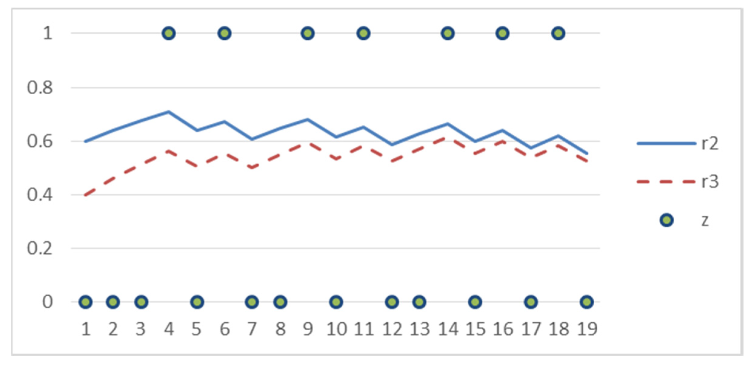
Example. Consider an illustrative example of three agents with the initial types , , and Assume that the cognitive dissonance effect is absent (ci = 0, ). The first agent does not change his type: d1 = 0. The second and third agents are anti-conformists: d2 = 0.1 and d3 = 0.1. The dynamics of the agents’ types (second and third agents) and activity result (unstable!) are shown in Figure 2.
6. Model of Informational Confrontation
Consider three agents: the first and second agents perform informational control (choose controls as their actions), affecting (due to the informational influence) the type (internal state—opinion or belief) of the third agent. The common activity result for all agents is the state of the third agent by a terminal period T.
Let the opinion rt of the third agent in period t be a linear combination of his opinion and the opinions of the first and second agents in the previous period: . (All opinions have the range [0, 1).)
Assume that the goals of the first and second agents are opposite (the first one is interested in turning rt to state “0”, while the second one—to state “1”) and their states are invariable: , . Interpretations of agents states are the same as in Section 4 above.
If, in each period, the agents exchanged their opinions (true states), the opinion dynamics would be .
The controls of the first and second agents are to inform the third agent about their opinions in some periods. Therefore, we have:
The sets of admissible actions have the form , (such controls are called binary). Then = . Substituting , , we arrive at the following state dynamics of the third agent:
where and r0 is a given initial state. (Also, see the expressions (3) and (7) above.) Let the first agent be interested in minimizing the terminal state rT, whereas the second in maximizing it. Note that the consumption of resources and other costs are not included in the goal functions.
In a practical interpretation, the state of the third agent (his opinion, belief, or attitude towards some issue or phenomenon) is reduced by the first agent and increased by the second. There is an informational confrontation between the first and second agents, described by game theory. In the dynamic case considered below, we have a differential game; static models of informational confrontation and models of repeated games can be found in [28,29].
According to (12), the combinations, presented in Table 3, are possible in each period.
In the latter case, the state of the third agent has a nonnegative increment if .
A differential counterpart of the difference Equation (12) has the form:
Assume that the actions of the first and second agents are subjected to the integral resource constraints (i.e., resources for customized publications in mass media or posts in social media, advertising costs, etc.)
First, let us study several special cases.
Case 1 (control applied by the first agent only). Substituting or (and) into (13), we obtain the differential equation . Due to the constraint (14), the solution yields the estimate of the terminal state, which is independent of the trajectory .
Case 2 (control applied by the second agent only). Substituting or (and) into (13), we obtain the differential equation . Due to the constraint (14), the solution yields the estimate of the terminal state, which is independent of the trajectory .
Case 3 (unlimited resources, both agents choose the actions , in all periods). In this case, Equation (13) takes the form:
The solution is given by:
The characteristic time is , and the asymptotic value is .
Now, we return to the general case (13). Let , , denote the resource consumption of agent i by a period t, representing a nondecreasing function of time. The choice of these functions by the first and second agents can be treated as their strategies.
The solution of Equation (13) is given by:
Consider the differential zero-sum two-person (antagonistic) game in normal form [32,33] of the first two agents. At the initial time instant of this game, the first and second agents choose their open-loop strategies and , respectively, once, simultaneously, and independently of one another.
Further analysis will be restricted to the class of strategies with a single switch. In this class, at the initial time instant, the first and second agents simultaneously and independently choose some instants t1 and t2, respectively, when they start consuming their resource (apply controls) until complete exhaustion. Therefore, the open-loop strategies have the form:
The functional (17) monotonically decreases in and increases in . Hence, the first and second agents benefit from consuming the entire resource, and consequently, and .
There are four possible relations among the parameters and
The first relation: (both agents have enough resources).
Here the Nash equilibrium strategies are: , due to the monotonicity mentioned above.
The second and third relations: for some , and .
Here, for agent i, the optimal strategy is: . For agent (3 − i), the optimal switching instant is the solution of a scalar optimization problem. The case is of practical interest. Note that the binary control is optimal under the constraints , due to the linearity of (13) in the controls.
The fourth relation: (both agents lack resources).
Here the agents play a complete game. If , then the equilibrium of this game is . Therefore, both agents start spending resources as late as possible, and the terminal value is . The same pair of strategies will be an equilibrium for (when the quantities of resources are such that the controls are short-term on the scale of the period T). Practical interpretation is “save all reserves until the last decisive moment”.
Hence, the results of this section give optimal strategies of the first two agents and characterize the equilibrium of their informational confrontation.
7. Conclusions
The main result is a general model (1)–(3) of joint dynamics of agents’ actions and internal states, depending as on previous actions and states, as on the environment and the results of activity (see Figure 1). It allows combining methods and approaches of various decision-making paradigms, game theory, and social psychology to external and internal aspects of collective strategic decision-making.
Many known models and results of the above-mentioned scientific domains—reflecting the effects of consensus, threshold behavior, cognitive dissonance, informational influence, control, and confrontation—turn out to be the particular cases of the general model.
Three main directions seem prospective for future researches. First, the analysis of the general models in order to explore maximally general but analytical conditions for equilibrium existence, uniqueness, and its comparative statics. Second, generating new particular/applied models of collective activity and organizational behavior and management, taking into account not only “economical” rationality but psychological aspects as well. The third direction is the field of model identification and verification to put them closer to reality and practical applications.
Funding
This research received no external funding.
Data Availability Statement
Not applicable.
Conflicts of Interest
The author declares no conflict of interest.
References
- Novikov, D. Control, activity, personality. Adv. Syst. Sci. Appl. 2020, 20, 113–135. [Google Scholar]
- Novikov, D. Dynamics models of mental and behavioral components of activity in collective decision-making. Large-Scale Syst. Control 2020, 85, 206–237. [Google Scholar]
- Belov, M.; Novikov, D. Methodology of Complex Activity: Foundations of Understanding and Modelling; Springer: Berlin/Heidelberg, Germany, 2020. [Google Scholar]
- Banisch, S.; Olbrich, E. Opinion polarization by learning from social feedback. J. Math. Sociol. 2019, 43, 76–103. [Google Scholar] [CrossRef]
- Flache, A.; MäS, M.; Feliciani, T.; Chattoe-Brown, E.; Deffuant, G.; Huet, S.; Lorenz, J. Models of social influence: Towards the next frontiers. J. Artif. Soc. Soc. Simul. 2017, 20, 31. [Google Scholar] [CrossRef] [Green Version]
- Neumann, J.; Morgenstern, O. Theory of Games and Economic Behavior; Princeton University Press: Princeton, NJ, USA, 1944. [Google Scholar]
- Fishburn, P. Utility Theory for Decision Making; R. E. Krieger Pub. Co: London, UK, 1979. [Google Scholar]
- Myerson, R. Game Theory: Analysis of Conflict; Harvard University Press: London, UK, 1991. [Google Scholar]
- Heckelman, J.; Miller, N. Handbook of Social Choice and Voting; Edward Elgar Publishing: London, UK.
- Granovetter, M. Threshold models of collective behavior. Am. J. Sociol. 1978, 83, 1420–1443. [Google Scholar] [CrossRef] [Green Version]
- Schelling, T. Micromotives and Macrobehavior; Norton & Co Ltd.: London, UK, 1978. [Google Scholar]
- Dhami, S. The Foundations of Behavioral Economic Analysis; Oxford University Press: Oxford, UK, 2016. [Google Scholar]
- Myers, D. Social Psychology, 12th ed.; McGraw-Hill: Columbus, OH, USA, 2012. [Google Scholar]
- Perloff, R. The Dynamics of Persuasion, 6th ed.; Routledge: New York, NY, USA, 2017. [Google Scholar]
- Zimbardo, P.; Leippe, M. Psychology of Attitude Change and Social Influence; McGraw-Hill: Columbus, OH, USA, 1991. [Google Scholar]
- Cialdini, R. Influence: Theory and Practice, 5th ed.; Pearson: London, UK, 2008. [Google Scholar]
- Sage. The Sage Handbook of Personality Theory and Assessment. Vol. 1. Personality Theories and Models; Sage Books: Los Angeles, CA, USA, 2008. [Google Scholar]
- Schultz, D.; Schultz, S. Theories of Personality, 11th ed.; Cengage Learning: Boston, MA, USA, 2016. [Google Scholar]
- Feist, J.; Feist, G. Theories of Personality, 9th ed.; McGraw-Hill Education: New York, NY, USA, 2017. [Google Scholar]
- Allbaracin, D.; Shavitt, S. Attitudes and attitude change. Annu. Rev. Psychol. 2018, 69, 299–327. [Google Scholar] [CrossRef] [PubMed]
- Hunter, J.; Danes, J.; Cohen, S. Mathematical Models of Attitude Change; Academic Press: Orlando, FL, USA, 1984. [Google Scholar]
- Xia, H.; Wang, H.; Xuan, Z. Opinion dynamics: A multidisciplinary review and perspective on future research. Int. J. Knowl. Syst. Sci. 2011, 2, 72–91. [Google Scholar] [CrossRef] [Green Version]
- Shoham, Y.; Leyton-Brown, K. Multiagent Systems: Algorithmic, Game-Theoretical and Logical Foundations; Cambridge University Press: Cambridge, UK, 2009. [Google Scholar]
- Yakouda, M.; Abbel, W. Multi-Agent System: A Two-Level BDI Model Integrating Theory of Mind. Int. J. Eng. Res. Technol. 2020, 9, 208–216. [Google Scholar]
- Burkov, V.; Goubko, M.; Kondrat’ev, V.; Korgin, N.; Novikov, D. Mechanism Design and Management: Mathematical Methods for Smart Organizations; Nova Science Publishers: New York, NY, USA, 2013. [Google Scholar]
- Novikov, D. Theory of Control in Organizations; Nova Science Publishing: New York, NY, USA, 2013. [Google Scholar]
- Belov, M.; Novikov, D. Optimal Enterprise: Structures, Processes and Mathematics of Knowledge, Technology and Human Capital; CRC Press: Boca Raton, FL, USA, 2021. [Google Scholar]
- Breer, V.; Novikov, D.; Rogatkin, A. Mob Control: Models of Threshold Collective Behavior; Springer: Berlin/Heidelberg, Germany, 2017. [Google Scholar]
- Chkhartishvili, A.; Gubanov, D.; Novikov, D. Social Networks: Models of Information Influence, Control and Confrontation; Springer: Berlin/Heidelberg, Germany, 2019. [Google Scholar]
- Belov, M.; Novikov, D. Models of Technologies; Springer: Berlin/Heidelberg, Germany, 2020. [Google Scholar]
- Minakowski, P.; Mucha, P.; Peszek, J. Density-induced consensus protocol. Math. Models Methods Appl. Sci. 2020, 30, 2389–2415. [Google Scholar] [CrossRef]
- Gorelov, M.; Kononenko, A. Dynamic models of conflicts. III. Hierarchical games. Autom. Remote Control. 2015, 76, 264–277. [Google Scholar] [CrossRef]
- Malsagov, M.; Ougolnitsky, G.; Usov, A. A differential Stackelberg game theoretic model of the promotion of innovations in universities. Adv. Syst. Sci. Appl. 2020, 20, 166–177. [Google Scholar]
Figure 1.
Structure of decision-making process [2].
Figure 1.
Structure of decision-making process [2].

Figure 2.
Dynamics of agents’ types and activity result in the example.


Table 1.
Decision-making factors and related scientific domains.
| Factor Scientific Domain | Utility | Action | Actionsof Others | Environment (and Results of Activity) | Internal State | History | Control |
|---|---|---|---|---|---|---|---|
| Individual decision-making [6,7] | +++ | ++ | ++ | + | + | ||
| Game theory [8], theory of collectivebehavior [9,10,11], behavioral economics [12] | ++ | +++ | +++ | + | + | + | + |
| Social psychology [13,14,15,16], Psychology of personality [17,18,19] Mathematical psychology [20,21,22] | + | ++ | + | ++ | +++ | + | + |
| Multi-agent systems [23,24] | +++ | + | ++ | ++ | + | + | |
| Control theory (of social and organizational systems) [25,26] | ++ | ++ | ++ | +++ | + | + | +++ |
Table 2.
Modifications of model (7).
| Modification | Control | Cognitive Dissonance | Conformity Behavior |
|---|---|---|---|
| 1 | − | − | − |
| 2 | + | − | − |
| 3 | − | + | − |
| 4 | − | − | + |
| 5 | + | + | − |
| 6 | + | − | + |
| 7 | − | + | + |
| 8 | + | + | + |
Table 3.
The combinations of each period.
| y1 = 0 | y2 = 0 | (the state of the third agent is invariable) |
| y1 = 1 | y2 = 0 | |
| y1 = 0 | y2 = 1 | |
| y1 = 1 | y2 = 1 |
Publisher’s Note: MDPI stays neutral with regard to jurisdictional claims in published maps and institutional affiliations. |
© 2021 by the author. Licensee MDPI, Basel, Switzerland. This article is an open access article distributed under the terms and conditions of the Creative Commons Attribution (CC BY) license (https://creativecommons.org/licenses/by/4.0/).
Share and Cite
MDPI and ACS Style
Novikov, D. Models of Strategic Decision-Making under Informational Control. Mathematics 2021, 9, 1889. https://0-doi-org.brum.beds.ac.uk/10.3390/math9161889
AMA Style
Novikov D. Models of Strategic Decision-Making under Informational Control. Mathematics. 2021; 9(16):1889. https://0-doi-org.brum.beds.ac.uk/10.3390/math9161889
Chicago/Turabian StyleNovikov, Dmitry. 2021. "Models of Strategic Decision-Making under Informational Control" Mathematics 9, no. 16: 1889. https://0-doi-org.brum.beds.ac.uk/10.3390/math9161889
Note that from the first issue of 2016, this journal uses article numbers instead of page numbers. See further details here.