
Modeling Proportion Data with Inflation by Using a Power-Skew-Normal/Logit Mixture Model


1
Departamento de Matemáticas y Estadística, Facultad de Ciencias Básicas, Universidad de Córdoba, Montería 230002, Colombia
2
Departamento de Matemáticas, Facultad de Ciencias Básicas, Universidad de Antofagasta, Antofagasta 1240000, Chile
*
Author to whom correspondence should be addressed.
†
These authors contributed equally to this work.
Mathematics 2021, 9(16), 1989; https://doi.org/10.3390/math9161989
Submission received: 30 June 2021
/
Revised: 7 August 2021
/
Accepted: 17 August 2021
/
Published: 20 August 2021
Abstract
:Rate or proportion data are modeled by using a regression model. The considered regression model can be used for studying phenomena with a response on the (0, 1), [0, 1), (0, 1], or [0, 1] intervals. To connect the response variable with the linear predictor in the regression model, we use a logit link function, which guarantees that the obtained prediction ranges between zero and one in the cases inflated at zero or one (or both). The model is complemented with the assumption that the errors follow a power-skew-normal distribution, resulting in a very flexible model, and with a non-singular information matrix, constituting an advantage over other existing models in the literature. To explain the probability of point mass at the values zero and/or one (inflated part), we used a polytomic logistic model with covariates. The results of two illustrations showed that the proposed model is a better alternative compared to widely known models in the literature.
1. Introduction
Statistical modeling to explain variables, such as the concentration of sulfur in the tissue in 100 g of leaves of a certain genotype of bean (measured by turbidimetric methods), the proportion of children killed by unknown causes in the main cities of a country, the proportion of deaths caused by smoking, the prevalence rate of a certain disease in a community, the proportion of votes in favor of a presidential candidate for reelection, the proportion of income spent on education, and, in general, any response variable on the unit interval as proportions, rates, or indices, has been studied by several researchers, highlighting the works of Paolino [1], Cribari-Neto and Vasconcellos [2], Kieschnick and Mccullough [3], Ferrari and Cribari-Neto [4], and Vasconcellos and Cribari-Neto [5].
Among the most recent works, we emphasize Ospina and Ferrari [6,7], Bayes et al. [8] and Martínez-Flórez et al. [9,10] who have presented extensions of the works mentioned above, some of them by incorporating a set of covariates to the model. Other works in this same area are those of Mazucheli et al. [11,12,13] and Menezes et al. [14], which extend the Birbaum–Saunders, gamma, Weibull, and logistic models, respectively, to situations of models able to fit datasets whose variables are on a unity interval. These families have proven to be a good alternative to the beta model of Ferrari and Cribari-Neto [4] and the Kumaraswamy distribution by [15].
The previously mentioned distributions used for modeling proportions, rates, and indices as well as their respective extensions have special characteristics from which is possible to decide if is a favorable option for fitting a particular dataset; usually, the asymmetry and kurtosis coefficients are the most used. Unquestionably, these measures are associated with certain parameters of each model; generally, the parameters to which we refer are linked to characteristics of shape and/or asymmetry or the kurtosis of the distribution. Some works include the case of unit variables that contain an excessive amount of zeros and/or ones, and they are known in the literature as inflated distributions in the values of zero or one. Some works for dealing with these situations have been proposed by Ospina and Ferrari [7] and Martínez-Flórez et al. [10], among others.
The main objective of this article is to propose a new class of regression models based on the power-skew-normal distribution, which are useful for fitting data with response on the unit interval. The new models allow taking into account possible excesses of the zero and/or one values of the response variable and are also able to capture different forms of the response distribution, as well as high (or low) degrees of asymmetry and kurtosis present in the data.
The rest of this paper is organized as follows: Section 2 presents some asymmetric distributions and its main characteristics. In Section 3, the power-skew-normal/logit model is introduced, and its main properties are discussed. In addition, the statistical inference is carried out by using the maximum likelihood method. Section 4 presents the unit-power-skew-normal model for fitting data on the interval. For this model, the maximum likelihood method is used to carry out the estimation of parameters. The score function and the elements of the observed information matrix are presented in detail. Section 5 presents the extension of the inflated unit-power-skew-normal model, which is an alternative to the inflated beta regression model. In particular, the log-UPSN model is studied. In Section 6, the doubly censored PSN model is presented, and the generalized two-part PSN model with covariates is studied as a particular case. Finally, in Section 7, two illustrative examples are reported and compared with several rival models.
2. Asymmetric Distributions
The study of families with flexible distributions capable of modeling different degrees of asymmetry and kurtosis has been of great interest in the recent statistical literature. Different works have been published, with initial works by Birnbaum [16], Lehmann [17], Roberts [18], and O’Hagan and Leonard [19] and more recently by Fernandez and Steel [20], Mudholkara and Hutson [21], Azzalini [22], Durrans [23], Gupta and Gupta [24], Arellano-Valle et al. [25,26], Gómez et al. [27], and Pewsey et al. [28]. Azzalini [22] introduces the skew-normal (SN) distribution by adding an extra parameter to the normal model. The inclusion of this new parameter allows for fitting data with high degrees of asymmetry. The probability density function (pdf) for the skew-normal model with location parameter and scale parameter is given by
where and . The functions and denote the pdf and cumulative distribution function (cdf) of the standard normal distribution. The model in (1) is denoted by , and the respective cdf is written as
where is the Owen function (see [29]). Another asymmetric model widely studied in the statistical literature is the named power-normal (PN), which was initially introduced by Durrans [23]. The PN model is sometimes denominated the generalized Gaussian distribution. Later, Gupta and Gupta [24,30] studied some statistical properties of the PN model, and they called it the exponential distribution. On the other hand, Pewsey et al. [28] studied the statistical inference of the PN model by using the maximum likelihood method; here, the authors deduce the expected information matrix, and they show the non-singularity of the matrix. The pdf of the location-scale version of the PN model is given by
where is a shape parameter, which contributes strongly to the kurtosis of the model. The model in (3) is denoted by , and the respective cdf is given by
An extension of the PN model which is capable of capturing greater ranges of asymmetry and kurtosis was proposed by Martínez-Flórez et al. [31]. This proposal, which is named the power-skew-normal (PSN) model, is originated by replacing the pdf and cdf of the normal distribution in the PN model by those of the SN model, that is, the PSN model contains both shape and asymmetry parameters. The pdf for the location-scale version of the PSN model is given by
where and . This is denoted by . One can observe that, for , the SN model is obtained, while for , the PN model is followed. The normal model is obtained when and , that is, the PSN model is more flexible than the normal, SN and PN models. If , then the cdf of X is given by
where is Owen’s function. For and values ranging in the interval, the asymmetry and kurtosis coefficients for the PSN model are and , respectively; these intervals contain the respective asymmetry and kurtosis coefficients of the SN and PN models (see Pewsey et al. [28]). The extensions for the positive data of the random variable X following the SN, PN or PSN models are obtained by applying the transformation , and they are denominated as a log-skew-normal (LSN) distribution, log-power-normal (LPN) distribution and log-power-skew-normal (LPSN) distribution, respectively (see Martínez-Flórez et al. [9,32], Mateus-Figueras and Pawlosky-Glanh [33]).
Asymmetric models have become very useful statistical tools for modeling censored or truncated data using covariates: see, for example, the log-gamma model by Moulton and Halsey [34], the log-skew-normal model of Chai and Bailey [35], the power-normal model by Martínez-Flórez et al. [9], and log-power-normal models by Martínez-Flórez et al. [9,32]. In this work, we extend the PSN model to the case of proportions, rates or indices data. The proposed extension is useful for modeling data with a response on the unit interval with an excess of zeros and/or ones and covariates to explain the response and the excess of zeros and/or ones.
3. The Power-Skew-Normal/Logit Mixture Model
The linear regression model with errors following a distribution was introduced and studied in detail by Martínez-Flórez et al. [32]. This model is expressed as
where is an unknown vector of regression coefficients, is a vector containing p known explanatory variables with , and for . It follows that
Since , it follows that ; therefore, it is necessary to correct the parameter in the form , where . Thus, it is obtained that , where . The ordinary least squares method can be used to obtain an estimate of the parameter vector , which can be used as an initial value in the maximum likelihood estimation process.
The main interest in this paper is centered on the case where the measured variable has a response on the unit interval, and the expected response or predicted value falls outside of this unit interval, which could lead to negative estimates without any interpretation or meaning. To avoid these inconveniences, the assumption of response variable Y being a linear function of the vector of explanatory variables is replaced by the assumption of a non-linear transformation of this set of variables. This model is obtained by assuming that the location parameter of the variable can be written as
where is a strictly monotonic link function whose second derivative exists. Two link functions widely used in practical situations that can be considered in (7) are the probit with , where is the cdf of the standard normal distribution, and the logit function given by . These two options lead to very similar results in the predicted values, with some exceptions for extreme values. For the ease of handling deductions, in this work, we opt for the logit function. Thus, in this case, we have
For the function in (8), the parameters are interpreted from the odds ratio between the odds of the prediction or mean when one of the variables is increased m units (keeping the rest of the explanatory variables fixed) and the odds without the increase. One can show that this quotient of odds ratios is given by , where is the parameter associated with the explanatory variable increased by m units. It follows that the distribution of the study variable is
From the model in (9), some special cases can be obtained; for example, if , the skew-normal-logit model is obtained, while, for , the exponential or alpha-power-logit case is followed. If and , it has the normal-logit model.
The parameter estimation of the PSN regression model on the unit interval with logit link function can be obtained by using the maximum likelihood method. The log-likelihood function obtained from a random sample of size n is given by
where for . To obtain the elements of the score function and the observed information matrix of the parameters , we use the fact that
where is given in (8). Then, the elements of the score function can be written in the form
where and . The scores equations are obtained by setting the elements of the score function equal to zero, that is, the first derivative of with respect to the parameters , , , and . By solving this system of equations, the maximum likelihood estimates are obtained. To maximize the log-likelihood function, it is necessary to use iterative numeric methods. Likewise, as in the standard case, the observed and expected Fisher information matrices are obtained as minus the Hessian matrix (the second derivative of with respect to the parameters) and the expected value of the elements of the observed information matrix, respectively. After some algebraic manipulations, it follows that the elements of the observed information matrix can be written in the form , and being the set of observations.
Letting and the elements are given by
Now, by letting and , and using numerical integration, the Fisher information matrix is given by
where with and
with . The determinant of the matrix is given by
Since is of full-column rank, and is a diagonal matrix, the rank of is the same as the , that is, the matrix is of full-column rank; therefore, will be full-rank and hence invertible, that is, its determinant is different from zero. Now, to find the last determinant, we write where ; this partition leads to expressing the matrix as a partitioned matrix, for which we can use the existing expressions of the matrix algebra to find the inverse of a partitioned matrix, that is, we can determine . With this result, it follows that, and, as for , , which leads to , concluding that that is, is non-singular, and therefore its rows and/or columns are linearly independent. Thus, the rows and/or columns of the information matrix are linearly independent, that is, . This leads to a non-singular matrix, because its columns (or rows) are linearly independent. Therefore, the regularity conditions are satisfied, and the known -property for the maximum likelihood estimators is satisfied for all and .
This important result further supports the hypothesis of singularity in the information matrix for the SN model for cases where the variable is a linear transformation of the location parameter. For other non-linear transformations, such as the asymmetric Birbaum–Saunders distributions studied by Vilca and Leiva-Sánchez [36], the asymmetric sinh-normal model of Leiva-Sánchez [37], and the asymmetric Birbaum–Saunders exponential distribution in Mattínez-Flórez et al. [38], the information matrices turned out to be non-singular.
4. Unit-Power-Skew-Normal Model
The unit-power-skew-normal (UPSN) model can be defined from the doubly truncated power-skew-normal (TPSN) distribution on the interval , which has a pdf given by
where
The properties of the doubly TPSN model can be studied from the properties of the truncated models. One can observe from Equation (14) that, if , the standard unit skew-normal-logit model is obtained, while, for , the standard unit exponential-logit or alpha-power-logit model is obtained. Finally, when and , the standard unit normal-logit model is followed.
The cdf of the TPSN model is given by
and the survival and Hazard functions are given by
respectively. The moments of the TPSN model can be calculated by the expression
where
being the inverse function of . The estimates of the parameters of the doubly TPSN-logit model (14) considering a set of covariates can be obtained by using the maximum likelihood method. The log-likelihood function for estimating is given by
where , , are defined in (15). The scores equations are obtained by setting the first derivative of with respect to the parameters , and , equal to zero. The solution of the resulting system of equations leads to maximum likelihood estimates, which is maximized by using iterative numeric methods.
The covariance matrix and standard errors for the TPSN model can be obtained from the inverse of the observed information matrix, given by minus the second derivative of the log-likelihood function in Equation (20) with respect to the parameters of the model, , , , and . Then, the observed information matrix of the truncated unit PSN-logit model can be found from the elements of the matrix of the unit PSN-logit model; these elements can be written as
where
In addition, for
it follows that
According to the results found for the the PSN-logit model, the information matrix of the model is non-singular; therefore, for large sample sizes, we have
That is, the vector of the estimators is consistent and has a normal asymptotic distribution, with covariance matrix being the inverse of the Fisher information matrix. In practice, since the matrix is consistent for , then we can take as the covariance matrix of the vector of estimators of the standard unit PSN-logit regression model.
5. Inflated Unit-Power-Skew-Normal Model
Ospina and Ferrari [6] introduced the zero-one inflated beta (BIZU) model, which is a mixture between a random variable with Bernoulli distribution with parameter , for and a reparameterized beta distribution of parameters and . Particular cases of this model follow for the situations of a unique inflated extreme value (zero or one) called BIZ and BIU, respectively. These ideas can be extended to the truncated unit-PSN model.
By considering that the mass point at value zero can be modeled by a Bernoulli random variable with parameter , namely and the responses between zero and one can be modeled by the truncated centered unit-power-skew-normal distribution, with parameter , the random variable on the unit interval then follows a truncated unit distribution inflated at zero and one, with parameters if its pdf is represented by the mixture
where . By the construction shown in the previous pdf, it holds that and , being the mixture parameter. For w, , and defined as in Equation (15), the cdf of Y can be written as
Considering the parameterization and where , the above model can be written in the form
From this model, inflation at zero is obtained by taking , and inflation at one follows by taking . Now, we introduce covariates in the model. For the discrete part, we assume that the responses in zero and one can be explained by the covariate vectors and , respectively. Then, following the construction of a logistic model with polytomous response, it is obtained that
where and are vectors of unknown parameters associated with the covariate vectors and , respectively. For the continuous part, we continue assuming a truncated centered unit-PSN model, with parameters , defined in (14). One can show that the log-likelihood function for the parameters vector , given , , , and , can be written in the form
where
and is defined in Equation (20).
This guarantees that the parameter estimates can be obtained in separate forms. The score functions and the observed information matrix are obtained by differentiating the log-likelihood function once and twice, with respect to the parameters, respectively. The fact that the log-likelihood function can be broken down into two independent components implies that the Fisher information matrix is a diagonal block, that is, it can be written as
where is related to the discrete part and to the set of parameters of the continuous part. This matrix coincides with the respective matrix for the previous case of the model for the standard on interval .
The elements of the observed information matrix for the discrete part are presented in Appendix A. Taking the expected value to these elements, the Fisher information matrix is obtained. Likewise, given the properties of the inverse of a diagonal matrix, one can conclude that the covariance matrix of the estimators vector can be written as
Confidence intervals for with confidence coefficient can be obtained as . Taking , the inflated model at zero is followed, UPSNIZ, and taking , the inflated model at one is followed, UPSNIU
The Log-UPSN Model
In some cases, the random variable does not follow a distribution; however, the random variable can have a distribution. In those cases, it is said that the random variable follows a truncated log-unit-PSN model, and its pdf is given by
where
for . is used instead of due to the non-existence of the logarithm at the point . In the cases with covariates, it holds that
where This new model is denoted by . For in (25), is replaced by which is defined in (8).
The estimation of the parameters follows the same routine as in the case of the UPSN model; likewise, the information matrix of this model can be obtained from the information matrix of the UPSN model. It is enough to change to in the respective expressions. For this model, in the case of inflation at zero and/or one, that is, in the intervals, , , and are used for the discrete part—a random variable binomial under a logit link function, similar to the case of the UPSN model.
6. Doubly Censored PSN Model
In this section, the model given by Moulton and Halsey [39] is generalized to the case of a mixture model for two limit points, lower and upper. One of the first models for the fit of the mixture between a discrete and a continuous random variable was proposed by Cragg [40], often called the two-part model. Under the Cragg model, the pdf of can be formally written as , where is the probability that determines the relative contribution made by the point mass to the general mixture distribution, f is a density function with positive support, if and if . In this model, the two components are determined by different stochastic processes, so a positive response is necessarily reached from f. On the other hand, a zero comes from the point mass distribution. This model, however, does not consider the situation of a lower limit and that part of the observations may be below the lower limit.
We extend Cragg’s model [40] to the case of the doubly censored and centered power-skew-normal model. A random variable is said to be doubly censored when measurements above the upper limit of detection and below the lower limit of detection are taken as those values. The lower and upper detection limits are specified by the researcher and generally depend on the measuring device used to produce the measurements. For our particular case, the lower and upper detection limits are given by and , respectively. For , a random sample where, for , the doubly censored random variable PSN between zero and one is defined as
We use the notation . The contribution of the uncensored observations to the likelihood function, , is given by the density function
On the other hand, the contribution of the censored observations at is given by
while the contribution of the censored observations at is given by
The parameters estimation of the DCPSN model can be achieved by maximizing the log-likelihood function given by
Generalized Two-Part PSN Model with Covariates
Moulton and Halsey [39] generalize the two-part model by explicitly allowing the possibility that some limited responses are the result of the censoring interval of f. This means that an observed zero can be a realization from the point mass distribution or partial observation of f with a critical value not precisely known, but close to for a small prespecified constant T, the lower detection limit.
Formally,
where F is the cdf associated with the f density function. In many studies, . Therefore, a large family of mixed models can be generated by varying the basic density f and the corresponding link function . One can see that if , for , the Moulton and Halsey [39] model is reduced to the Tobit model.
The two-part model by Moulton and Halsey [39] is extended to the situations of doubly censored responses. If denotes the proportion of observations below the lower detection limit, , and denotes the proportion of observations above the upper detection limit, , then the doubly censored model can be defined from the pdf.
with , as in the generalized doubly censored model of Cragg [40], and is the distribution of the truncated PSN model defined on the interval. Some mixture models have been used in practical applications in different fields such as biology, economy, agriculture, etc.—to mention a few, the probit/truncated-normal, logit/log-normal, logit/log gamma and probit/log-skew-normal mixture models (see Chai and Bailey [35] and Martínez-Flórez et al. [9]).
We consider an extension of the two-part generalized model for the situations of logit/doubly censored power-skew-normal model, together with covariates in each part of the model. Denoting and as auxiliary covariates for the discrete part at zero and one, respectively; denoting a set of covariates for the continuous part at ; and letting be the proportion of observations below zero, with being the lower detection limit and the proportion of observations above one, with as the upper detection limit, then the extension of the Moulton and Halsey [39] model for the case of the doubly censored PSN model is represented by the density function
where and are the point mass probabilities at the values zero and one, respectively, and , and are defined as in the equations given in (15). For modeling the responses at the mass points and , we define a binomial random variable with logit link function and polytomous response as defined in Equations (21) to (23).
A more general model, where only a proportion, , with , of censored observations come from the censored PSN model and the rest of the censored observations, say , are located below or at the point , and are located above or at the point , can be obtained from the model in Expression (29).
The log-likelihood function for estimating the parameter vector of the model, given , is
To obtain the information matrix, we proceed as in the case of the truncated UPSN model in the interval . Again, the right-censored or left-censored cases will be special cases of this model for and , respectively. The log-doubly censored case is constructed in the same way as was done for the truncated UPSN model, that is, by taking
with , , and defined as in (25).
7. Examples
In this section, we present two examples which allow us to illustrate the applicability of the proposed models.
7.1. Example 1
The first example is related to the household expenditure on food of 38 households taken from Griffiths et al. [41]; this dataset is available in the betareg library of the R Development Core Team [42]. The response variable is the relationship or rate of food/income, that is, the proportion of the family income spent on food, while the explanatory variables are: the family income mentioned above and the number of people living in the household. Ferrari and Cribari-Neto [4] modeled this set of variables through the beta regression model; therefore, we will implement the fit of the proportion of family income spent on food, explained through the covariates family income and number of people living at home, using PSN, SN, PN, and normal families of distributions, by using a logit link function. Likewise, we will fit the truncated PSN model with a logit link function. The estimation of the parameters for the previously mentioned models was carried out via maximum likelihood by using the optim function of R Development Core Team [42]. To compare the distributions in question, the AIC criteria by Akaike [43] and the corrected AIC (AICC) of Cavanaugh [44] were used. The criteria are defined by
where p is the number of parameters of the model in question. The maximum likelihood estimates, with standard errors in parentheses, are presented in Table 1. According to the results shown by the AIC and AICC criteria, the best fit is the truncated PSN-logit (TPSNL), followed by the PSN and SN models with logit link function.
We now compare the normal-logit (NL) model with the PSN-logit (PSNL) model through a hypothesis test.
Using the likelihood ratio statistic,
where denotes the likelihood function, we obtain
which is greater than the value of the . Thus, the PSN-logit model is a good alternative for fitting the dataset. The PSN-logit model is also compared to the PN-logit (PNL) model and the SN-logit (SNL) model by the hypothesis tests
respectively, using the likelihood ratio statistics
The numerical results were
which is greater than . The TPSNL model showed a better fit to the data compared to the other considered models.
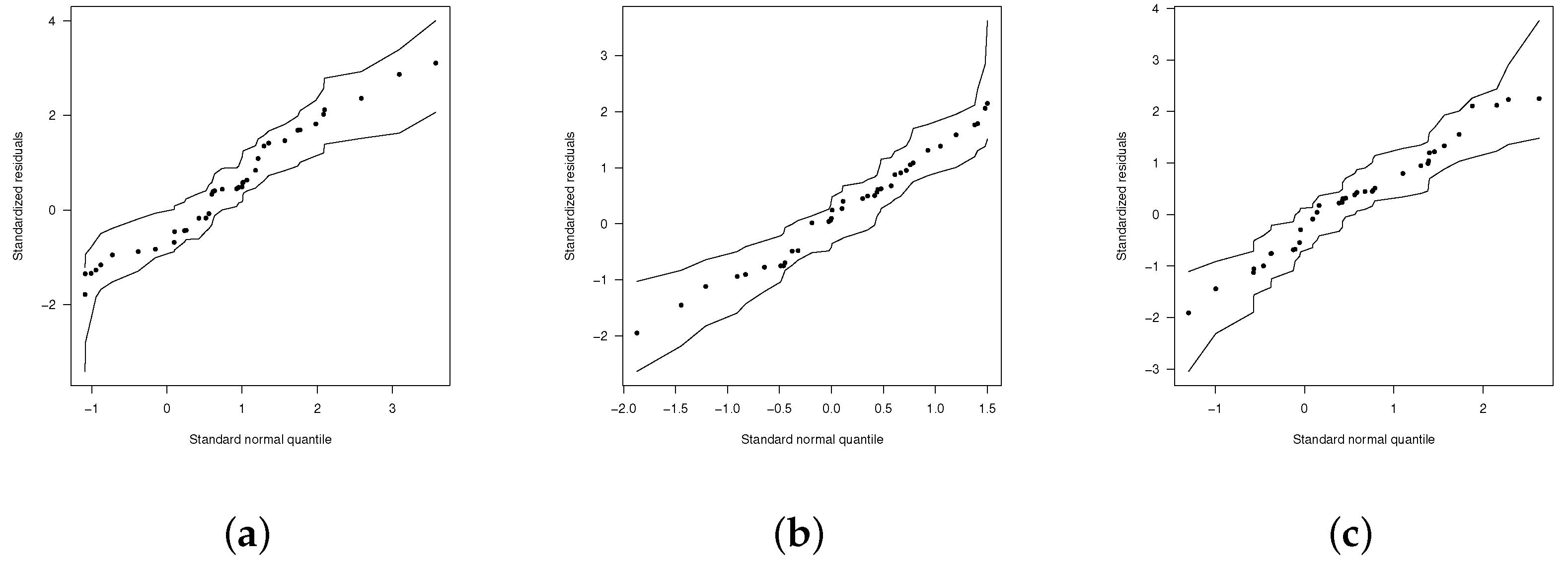
The transformed martingale residuals , introduced by Barros et al. [45], were considered with the goal to identify atypical observations and/or model misspecification. The transformed martingale residuals are defined by
where is the martingale residual introduced by Ortega et al. [46]; is an indicator function of the censorship of the ith observation with if the ith observation is censored and if the ith observation is uncensored; is the sign function; and represents the survival function evaluated at , where are the MLE for .
The plots with a generated envelope for the SN, PSN, and PSNT models are presented in Figure 1a–c. The graphs show that the PSN and PSNT regression models with logit link function present good fits, compared to the rest of the fitted regression models.
7.2. Example 2
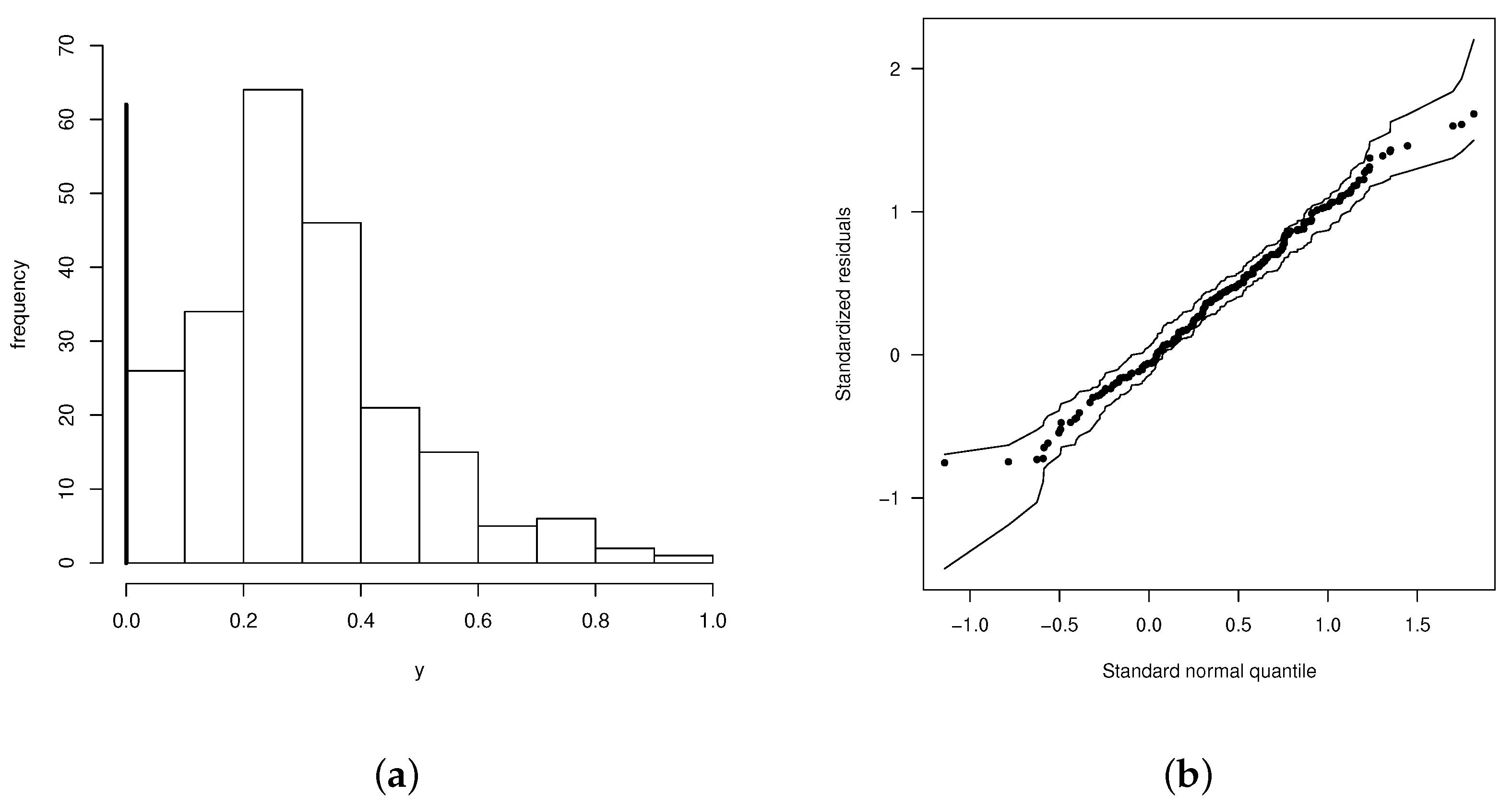
In the second example, we consider a dataset referring to the broadcasting of cable television in the USA. The data correspond to 282 communities that are essentially individual franchise areas with cable television allocation. The data were taken from The Federal Communications Commission (FCC) and are described in detail in Appendix E of FCC 93–177 [47]. The variable of interest, Y, is the proportion of households with cable television that purchase additional services.
The explanatory variables are: the logarithm of the average income in the franchise (lin) given in thousands of dollars; the percentage of children in the franchise (child); the number of channels with local signal (ltv); and (=) the age in years of the cable television system (agehe). This dataset is inflated to zero, 68 zeros, which corresponds to 21.98% of the observations, that is, the dataset is left censored. A graph of the response variable proportion of households with cable television that purchase additional services can be seen in Figure 2a. For this set of variables, the beta zero inflated (BIZ) linear regression model, the truncated PSN inflated at zero (PSNIZ) linear regression model, and the generalized two-part PSN model were fitted with detection limit at that is, zero-censored (CGPSN), these last two had a logit link function between zero and one, . After fitting each of these models, it was found that the significant variables were the logarithm of income (), for the component in (0,1), and the variable years of age of the cable television system (), for the censored part at The estimates of the parameters and the fitted models are found in Table 2. According to the AIC and AICC criteria, the CGPSN and PSNIZ models present a good fit compared to the BIZ model.
The graphs with envelopes generated for the BIZ, PSNIZ, and GCPSN models are found in Figure 2b and Figure 3a,b, which show that the PSNIZ and CGPSN regression models with logit link present a good fit, compared to the BIZ model—that is to say that these models are new alternatives to fit variables of rate and proportions, such as the proportion of households with cable TV that acquire additional services.
8. Conclusions
In this paper, new regression models for fitting data on the intervals , , , or were proposed. The main statistical properties of the proposed models and the problem of the parameters’ estimation are studied in detail by using the maximum likelihood method. For the fitting regression model, which can explain the phenomena under study, such as rates or proportions, a logit link function was implemented, with which it is guaranteed that the prediction obtained by the model is between zero and one. The results show that the models present a non-singular information matrix, and the applications show great potential in the proposed models, are more flexible than certain rival models, and fit better to some real datasets.
Author Contributions
Conceptualization, G.M.-F., H.W.G. and R.T.-F.; Methodology, G.M.-F. and H.W.G.; Data curation, G.M.-F., H.W.G. and R.T.-F.; Formal analysis, G.M.-F., H.W.G. and R.T.-F.; Funding acquisition, H.W.G. and R.T.-F.; Investigation, G.M.-F., H.W.G. and R.T.-F.; Resources, G.M.-F., H.W.G. and R.T.-F.; Software, G.M.-F. and H.W.G.; Supervision, G.M.-F.; Validation, G.M.-F. and R.T.-F.; Visualization, G.M.-F., H.W.G. and R.T.-F.; Writing—original draft, G.M.-F., H.W.G. and R.T.-F.; Writing—review & editing, G.M.-F., H.W.G. and R.T.-F. All authors have read and agreed to the published version of the manuscript.
Funding
The research of H.W. Gómez was supported by Grant SEMILLERO UA-2021 (Chile). The research of R. Tovar-Falón and G. Martínez-Flórez was supported by the project: Resolución de Problemas de Situaciones Reales Usando Análisis Estadístico a través del Modelamiento Multidimensional de Tasas y Proporciones; Esquemas de Monitoreamiento para Datos Asimétricos no Normales y una Estrategia Didáctica para el Desarrollo del Pensamiento Lógico-Matemático, Universidad de Córdoba, (Colombia). Code FCB-05-19.
Institutional Review Board Statement
Not applicable.
Informed Consent Statement
Not applicable.
Data Availability Statement
Details about data available are given in Section 7.
Acknowledgments
G. Martínez-Flórez and R. Tovar-Falón acknowledge the support given by Universidad de Córdoba, Montería, Colombia.
Conflicts of Interest
The authors declare no conflict of interest.
Appendix A. Elements of the Observed Information Matrix for the Discrete Part of the Inflated UPSN Model
In this section, expressions for the elements of the observed information matrix for the discrete part of the inflated unit-power-skew-normal model are presented.
References
- Paolino, P. Maximum likelihood estimation of models with beta-distributed dependent variables. Political Anal. 2001, 9, 325–346. [Google Scholar] [CrossRef]
- Cribari-Neto, F.; Vasconcellos, K.L.P. Nearly unbiased maximum likelhood estimation for the beta distribution. J. Stat. Comput. Simul. 2002, 72, 107–118. [Google Scholar] [CrossRef]
- Kieschnick, R.; Mccullough, B.D. Regression analysis of variates observed on (0, 1). Stat. Model. 2003, 3, 193–213. [Google Scholar] [CrossRef] [Green Version]
- Ferrari, S.; Cribari-Neto, F. Beta regression for modelling rates and proportions. J. Appl. Stat. 2004, 31, 799–815. [Google Scholar] [CrossRef]
- Vasconcellos, K.L.P.; Cribari-Neto, F. Improved maximum likelihood estimation in a new class of beta regression models. Braz. J. Probab. Stat. 2005, 19, 13–31. [Google Scholar]
- Ospina, R.; Ferrari, S.L.P. Inflated beta distributions. Stat. Pap. 2010, 51, 111–126. [Google Scholar] [CrossRef] [Green Version]
- Ospina, R.; Ferrari, S.L.P. A general class of zero-or-one inflated beta regression models. Comput. Stat. Data Anal. 2012, 56, 1609–1623. [Google Scholar] [CrossRef] [Green Version]
- Bayes, C.; Bazan, J.; García, C. A new robust regression model for proportions. Bayesian Anal. 2012, 7, 841–866. [Google Scholar] [CrossRef]
- Martínez-Flórez, G.; Bolfarine, H.; Gómez, H.W. Asymmetric regression models with limited responses with an application to antibody response to vaccine. Biom. J. 2013, 55, 156–172. [Google Scholar] [CrossRef]
- Martínez-Flórez, G.; Bolfarine, H.; Gómez, H.W. Power-models for proportions with zero/one excess. Appl. Math. Inf. Sci. 2018, 12, 293–303. [Google Scholar] [CrossRef]
- Mazucheli, J.; Menezes, A.F.B.; Dey, S. The unit-Birnbaum-Saunders distribution with applications. Chil. J. Stat. 2018, 9, 47–57. [Google Scholar]
- Mazucheli, J.; Menezes, A.F.B.; Dey, S. Improved maximum-likelihood estimators for the parameters of the unit-gamma distribution. Commun. Stat.-Theory Methods 2018, 47, 3767–3778. [Google Scholar] [CrossRef]
- Mazucheli, J.; Menezes, A.F.B.; Ghitany, M.E. The unit-Weibull distribution and associated inference. J. Appl. Probab. Stat. 2018, 13, 1–22. [Google Scholar]
- Menezes, A.F.B.; Mazucheli, J.; Dey, S. The unit-logistic distribution: Different methods of estimation. Pesqui. Oper. 2018, 38, 555–578. [Google Scholar] [CrossRef]
- Kumaraswamy, P. A generalized probability density function for double-bounded random processes. J. Hydrol. 1980, 46, 79–88. [Google Scholar] [CrossRef]
- Birnbaum, Z.W. Effect of linear truncation on a multinormal population. Ann. Math. Statist. 1950, 21, 272–279. [Google Scholar] [CrossRef]
- Lehmann, E.L. The power of rank Tests. Ann. Math. Statist. 1953, 24, 23–243. [Google Scholar] [CrossRef]
- Roberts, C. A Correlation Model Useful in the Study of Twins. J. Am. Stat. Assoc. 1966, 61, 1184–1190. [Google Scholar] [CrossRef]
- O’Hagan, A.; Leonard, T. Bayes estimation subject to uncertainty about parameter constraints. Biometrika 1976, 63, 201–202. [Google Scholar] [CrossRef]
- Fernandez, C.; Steel, M. On bayesian modeling of fat tails and skewness. J. Am. Stat. Assoc. 1998, 93, 359–371. [Google Scholar]
- Mudholkara, G.S.; Hutson, A. The epsilon–skew–normal distribution for analyzing near-normal data. J. Stat. Plan. Inference 2000, 83, 291–309. [Google Scholar] [CrossRef]
- Azzalini, A. A class of distributions which includes the normal ones. Scand. J. Stat. 1985, 12, 171–178. [Google Scholar]
- Durrans, S.R. Distributions of fractional order statistics in hydrology. Water Resour. Res. 1992, 28, 1649–1655. [Google Scholar] [CrossRef]
- Gupta, R.C.; Gupta, R.D. Generalized skew normal model. Test 2004, 13, 501–524. [Google Scholar] [CrossRef]
- Arellano-Valle, R.B.; Gómez, H.W.; Quintana, F.A. A new class of skew-normal distributions. Commun. Stat.-Theory Methods 2004, 33, 1465–1480. [Google Scholar] [CrossRef]
- Arellano-Valle, R.B.; Gómez, H.W.; Quintana, F.A. Statistical inference for a general class of asymmetric distributions. J. Stat. Plan. Inference 2005, 128, 427–443. [Google Scholar] [CrossRef]
- Gómez, H.W.; Venegas, O.; Bolfarine, H. Skew-symmetric distributions generated by the distribution function of the normal distribution. Environmetrics 2007, 18, 395–407. [Google Scholar] [CrossRef] [Green Version]
- Pewsey, A.; Gómez, H.W.; Bolfarine, H. Likelihood-based inference for power distributions. Test 2012, 21, 775–789. [Google Scholar] [CrossRef]
- Owen, D.B. Tables for computing bi-variate normal probabilities. Ann. Math. Stat. 1956, 27, 1075–1090. [Google Scholar] [CrossRef]
- Gupta, R.D.; Gupta, R.C. Analyzing skewed data by power normal model. Test 2008, 17, 197–210. [Google Scholar] [CrossRef]
- Martínez-Flórez, G.; Bolfarine, H.; Gómez, H.W. Skew-normal alpha-power model. Statistics 2014, 48, 1414–1428. [Google Scholar] [CrossRef]
- Martínez-Flórez, G.; Bolfarine, H.; Gómez, H.W. The log alpha-power asymmetric distribution with application to air pollution. Environmetrics 2014, 25, 44–56. [Google Scholar] [CrossRef]
- Mateus-Figueras, G.; Pawlosky-Glanh, V. Una Alternativa a la Distribución Lognormal; Actas del XXVII Congreso Nacional de Estadística e Investigación Operativa (SEIO); Sociedad de Estadística e Investigación Operativa: Barcelona, Spain, 2003; pp. 1849–1858. [Google Scholar]
- Moulton, L.; Halsey, N.H. A mixed gamma model for regression analyses of quantitative assay data. Vaccine 1996, 14, 1154–1158. [Google Scholar] [CrossRef]
- Chai, H.S.; Bailey, K.R. Use of log-skew-normal distribution in analysis of continuous data with a discrete component at zero. Stat. Med. 2008, 27, 3643–3655. [Google Scholar] [CrossRef] [Green Version]
- Vilca-Labra, F.; Leiva-Sánchez, V. A new fatigue life model based on the family of skew-elliptical distributions. Commun. Stat.-Theory Methods 2006, 35, 229–244. [Google Scholar] [CrossRef]
- Leiva-Sánchez, V.; Vilca-Labra, F.; Balakrishnan, N.; Sanhueza, A. A skewed sinh-normal distribution and its properties and application to air pollution. Commun. Stat.-Theory Methods 2010, 36, 426–443. [Google Scholar] [CrossRef]
- Martínez-Flórez, G.; Bolfarine, H.; Gómez, Y.M.; Gómez, H.W. A unification of families of Birnbaum-Saunders distributions with applications. REVSTAT 2020, 18, 637–660. [Google Scholar]
- Moulton, L.H.; Halsey, N.H. A mixture model with detection limits for regression analyses of antibody response to vaccine. Biometrics 1995, 51, 1570–1578. [Google Scholar] [CrossRef] [PubMed]
- Cragg, J. Some statistical models for limited dependent variables with application to the demand for durable goods. Econometrica 1971, 39, 829–844. [Google Scholar] [CrossRef]
- Griffiths, W.E.; Hill, R.C.; Judge, G.G. Learning and Practicing Econometrics, 1st ed.; Wiley: Hoboken, NJ, USA, 1993. [Google Scholar]
- R Development Core Team. R: A Language and Environment for Statistical Computing; R Foundation for Statistical Computing: Vienna, Austria, 2017; Available online: http://www.R-project.org (accessed on 12 February 2021).
- Akaike, H. A new look at statistical model identification. IEEE Trans. Autom. Control 1995, AU-19, 716–722. [Google Scholar]
- Cavanaugh, J.E. Unifying the derivations for the Akaike and corrected Akaike information criteria. Stat. Probab. Lett. 1997, 33, 201–208. [Google Scholar] [CrossRef]
- Barros, M.; Paula, G.A.; Leiva, V. A new class of survival regression models with heavy-tailed errors: Robustness and diagnostics. Lifetime Data Anal. 2010, 14, 316–332. [Google Scholar] [CrossRef] [PubMed]
- Ortega, E.M.; Bolfarine, H.; Paula, G.A. Influence diagnostics in generalized log-gamma regression models. Comput. Stat. Data Anal. 2003, 42, 165–186. [Google Scholar] [CrossRef]
- Federal Communications Commission. Report and Order and Further Notice of Proposed Rulemaking; MM Docker 92-266 (3 May 1993); Federal Communications Commission: Washington, DC, USA, 1993; Volume FCC 93–177, p. 6134.
Figure 1.
Envelope graphs for : (a) SN-logit model, (b) PSN-logit, and (c) PSNT-Logit.

Figure 2.
(a) Histogram for the variable Y and (b) envelope graphics for , BIZ model.

Figure 3.
Envelope graphics for , (a) GCPSN-logit model, and (b) PSNIZ-logit model.


Table 1.
Parameter estimates (standard errors) with logit link function for the normal, Beta, SN, PN PSN, and TPSN regression models.
Table 1.
Parameter estimates (standard errors) with logit link function for the normal, Beta, SN, PN PSN, and TPSN regression models.
| Estimator | Beta | Normal-Logit | SN-Logit | PN-Logit | PSN-Logit | TPSNL |
|---|---|---|---|---|---|---|
| −0.6225 | −1.0665 | −1.2348 | −0.8717 | −1.1259 | −1.2810 | |
| (0.2238) | (0.2061) | (0.1123) | (0.1363) | (0.1995) | (0.1663) | |
| −0.0122 | 0.0997 | 0.1376 | 0.0995 | 0.1246 | 0.1376 | |
| (0.0030) | (0.0086) | (0.0114) | (0.0077) | (0.0179) | (0.0167) | |
| 0.1184 | −0.0258 | −0.0513 | −0.0266 | −0.0441 | −0.0488 | |
| (0.0353) | (0.0025) | (0.0050) | (0.0020) | (0.0071) | (0.0067) | |
| 35.610 | 0.0374 | 0.0232 | 0.0271 | 0.0189 | 0.0202 | |
| (8.080) | (0.0083) | (0.0021) | (0.0053) | (0.0031) | (0.0029) | |
| 6.4714 | 7.4719 | 7.8010 | ||||
| (0.9057) | (2.1724) | (1.7758) | ||||
| 0.3771 | 0.2814 | 0.3891 | ||||
| (0.1575) | (0.1463) | (0.1867) | ||||
| AIC | −82.66 | −132.42 | −150.30 | −129.77 | −152.54 | −153.73 |
| AICC | −78.78 | −128.55 | −145.59 | −125.06 | −146.81 | −148.00 |
Table 2.
Maximum likelihood estimates of the parameters for fitted models.
| BIZ | CGPSN | PSNIZ | |
|---|---|---|---|
| 1.7830 (0.0902) | 0.2444 (0.0293) | 0.2402 (0.0194) | |
| 3.3627 (1.4804) | 2.1795 (1.0192) | ||
| 0.2803 (0.2849) | 0.3592 (0.2804) | ||
| AIC | 121.95 | 112.75 | 111.91 |
| AICC | 124.26 | 115.43 | 114.57 |
Publisher’s Note: MDPI stays neutral with regard to jurisdictional claims in published maps and institutional affiliations. |
© 2021 by the authors. Licensee MDPI, Basel, Switzerland. This article is an open access article distributed under the terms and conditions of the Creative Commons Attribution (CC BY) license (https://creativecommons.org/licenses/by/4.0/).
Share and Cite
MDPI and ACS Style
Martínez-Flórez, G.; Gomez, H.W.; Tovar-Falón, R. Modeling Proportion Data with Inflation by Using a Power-Skew-Normal/Logit Mixture Model. Mathematics 2021, 9, 1989. https://0-doi-org.brum.beds.ac.uk/10.3390/math9161989
AMA Style
Martínez-Flórez G, Gomez HW, Tovar-Falón R. Modeling Proportion Data with Inflation by Using a Power-Skew-Normal/Logit Mixture Model. Mathematics. 2021; 9(16):1989. https://0-doi-org.brum.beds.ac.uk/10.3390/math9161989
Chicago/Turabian StyleMartínez-Flórez, Guillermo, Hector W. Gomez, and Roger Tovar-Falón. 2021. "Modeling Proportion Data with Inflation by Using a Power-Skew-Normal/Logit Mixture Model" Mathematics 9, no. 16: 1989. https://0-doi-org.brum.beds.ac.uk/10.3390/math9161989
Note that from the first issue of 2016, this journal uses article numbers instead of page numbers. See further details here.