On the Poisson Stability to Study a Fourth-Order Dynamical System with Quadratic Nonlinearities

Abstract

This article discusses the search procedure for Poincaré recurrences to classify solutions on an attractor of a fourth-order nonlinear dynamical system, using a previously developed high-precision numerical method. For the resulting limiting solution, the Lyapunov exponents are calculated, using the modified Benettin’s algorithm to study the stability of the found regime and confirm the type of attractor.

1. Introduction

As it is known [1], the calculation of the Lyapunov exponents is used for the classification of attractors of dynamical systems. The combinations of signs of such values determine the attractor type: an equilibrium position, limit cycle, multidimensional torus or strange attractor. The dynamics of the corresponding solutions are called static, periodic, quasiperiodic, or chaotic. The computational procedure for determining the Lyapunov exponents is mainly based on Benettin’s algorithm [2]. However, in [3,4] the points of limiting solutions were investigated for the Poisson stability, which made it possible to understand whether we have a quasiperiodic or chaotic regime. In [4], it was done for the Jafari–Sprott system [5].

It is noteworthy [6] that a point y of the phase space is called positively Poisson stable ($P^{+}$) if for any neighborhood U of the point y and for any $T_P>0$, there is a time value $t\ge T_P$ for which the trajectory of the dynamical system enters into the neighborhood U. Similarly, if there is $t\le -T_P$ such that the trajectory enters into the neighborhood U, then the point y is negatively Poisson stable ($P^{-}$). A point is called Poisson stable if it is $P^{+}$ and $P^{-}$–stable.

The boundedness of the limiting solutions of dissipative systems implies [6,7,8,9,10] that any steady-state oscillation mode is described by Poisson-stable trajectories. This also applies to dynamical chaos. A trajectory different from the equilibrium position is said to be Poisson stable if it verifies the property of returning in an arbitrarily small $\epsilon$-neighborhood of each of its points an infinite number of times. Such returns are called the Poincaré recurrences. In [10] (p. 146), the author notes that “the study of the statistics of the Poincaré recurrences is a powerful tool for the analysis and classification of dynamic modes. Apparently, the potentialities of this approach have not yet been fully exhausted in modern nonlinear dynamics”. For example, the returns follow one another regularly for quasiperiodic regimes. Then, [10] (p. 145) “the dynamic chaos is a situation when the Poincaré recurrences to the $\epsilon$-neighborhood of the initial point do not show regularity, the time interval between two successive returns turns out to be different each time, and some statistical distribution of the times of return is arised” [11,12]. An example of the Poincaré recurrences analysis based on the Kac’s theorem [13,14,15,16,17,18] for a discrete dynamical system with a chaotic non-hyperbolic attractor is given in [16].

As it is known, for the most of dissipative systems, the formulas for a general solution of the system in a class of any known functions with well-studied properties have not yet been found. Therefore, numerical methods are used. The use of classical numerical methods (such as the Euler method, Runge–Kutta 4th order method, Adams methods, etc.) for constructing approximate solutions in attractors of dynamical systems leads to significant errors over large sections of time, due to the instability of the studied chaotic regimes. In general, the problem of numerical modeling with control of the accuracy of obtained solution and the choice of a platform for computer implementation is relevant today [19] since small errors introduced at each integration step cause exponential divergence of close trajectories. More recently, the numerical FGBFI method (Firmly Grounded Backward–Forward Integration) was proposed in [3,4,20], based on the power series method for dynamical systems with quadratic nonlinearities. The main advantages of this method are as follows:

• The recurrence relations are obtained for calculating the coefficients of the expansion of solutions in a power series for any dynamical system with quadratic nonlinearities in a general form;
• The convergence of the power series is studied. A simple formula for calculations is derived (in comparison with that of [21] obtained in the known literature) for calculating the length of the integration step in a general form;
• The criteria for checking the accuracy of the approximate solution are obtained. The control of the accuracy and configuration of the approximate solution of a dynamical system uses forward and backward time, which makes the numerical method reliable (degrees of piecewise polynomials, the value of the maximum integration step, etc.);
• The FGBFI method allows to construct high-precision approximations to non-extendable solutions of a system of autonomous differential equations with a quadratic right-hand side, like, for instance, the system of the following form:

  $$\dot{x}=1+x^2.$$
  In this case, the numerical solution computed with FGBFI will never cross the asymptote and will approach it arbitrarily closely.

Thus, it is a high-precision method for constructing the trajectory arc of the system for any time interval. This makes it possible to track the Poincaré recurrences to any neighborhood of the trajectory points since the resulting computational error can be smaller than the radius of the monitored neighborhoods.

This article considers a fourth-order dissipative system [22] in which, in the opinion of its authors, there is hyperchaos. The goals of the research are as follows: (1) to find the Poincaré recurrences in the attractor of this system for the approximate solutions obtained by the FGBFI method and to analyze the statistics of return times; and (2) to apply the modified Benettin’s algorithm [20] to refine the computation of the Lyapunov exponents.

2. Bohr’s Almost Periodic Functions

It is noteworthy [23] (pp. 368, 418, 419) that the function (trajectory of a dynamical system) $F\left(t\right)\in {\mathbb{R}}^n$ is called Bohr’s almost periodic in the sense that, if for any $\epsilon >0$ there exists a relatively dense set of almost periods ${\tau }_F={\tau }_F\left(\epsilon \right)$ of the function $F\left(t\right)$ with $\epsilon$-accuracy, i.e., there is the positive number $L=L\left(\epsilon \right)$ such that any interval $[\alpha ;\alpha +L]$ contains at least one number ${\tau }_F$ for which the inequality

$$\left|F(t+{\tau }_F)-F\left(t\right)\right|<\epsilon$$

holds at $t\in \mathbb{R}$. Note that for an almost periodic function (and, in general, for a Poisson stable trajectory), different from a periodic function, with decreasing number $\epsilon$, the number $L\left(\epsilon \right)$ must increase indefinitely; otherwise, the function would be periodic.

Usually (see, for example [10]) in nonlinear dynamics, almost periodic functions are called quasiperiodic.

Note an important theorem in the theory of dynamical systems [10] (p. 147): if a non-periodic trajectory is Poisson and Lyapunov stable, then it is almost periodic.

Since we will be investigating the Poincaré recurrences, it is noteworthy that for an almost periodic trajectory (as follows from the above definition), such returns must form a relatively dense set. An example of a sequence that is not a relatively dense set is the following:

$$0,1^2,2^2,3^2,\dots ,$$

since

$$\underset{q}{sup}|{(q+1)}^2-q^2|=\infty ,$$

i.e., in the given example, the distance between neighboring elements grows with the growth of q. A similar situation was observed in a numerical experiment for the Poincaré recurrences in the case of a chaotic solution of the Chen system [3].

3. Dissipative System of the Fourth Order

Let us consider a fourth-order system [22]:

$$\left\{\begin{array}{c}{\dot{x}}_1=a{x}_2-a{x}_1-e{x}_4,\hfill \\ {\dot{x}}_2=b{x}_1-x_2-x_1{x}_3-f{x}_4,\hfill \\ {\dot{x}}_3=x_1{x}_2-c{x}_3,\hfill \\ {\dot{x}}_4=k{x}_2{x}_3-d{x}_4,\hfill \end{array}\right.$$

(1)

where a, b, c, d, e, f and k are positive parameters. The divergence of the vector field G defined by the right-hand side of the system (1) is equal to

$$divG=-(a+1+c+d)<0.$$

Then, the system (1) is dissipative. Hence, there is the ball $B_a\subset {\mathbb{R}}^4$, into which each trajectory of the system (1) is immersed forever, after a while. Therefore, there is a limit set (attractor) such that all trajectories of the dynamical system are attracted when $t\to \infty$ [6].

Let us investigate the dynamics of the system (1) for the values of the parameters $a=7$, $b=50$, $c=3$, $d=10$, $e=5$, $f=5$ and $k=1.5$. In this case, it is possible to determine the position and radius of the ball $B_a$ from the data obtained in [22]. Additionally, in this article, the Lyapunov exponents are determined as $L{E}_1=2.1040$, $L{E}_2=0.3563$, $L{E}_3=0$ and $L{E}_4=-23.4508$, indicating a hyperchaos in the system (1). Therefore, its solutions are highly unstable, which requires the use of special numerical procedures for large time intervals.

Let us consider the application of the FGBFI method for constructing approximations to the solutions of the system (1), using high-precision calculations.

4. The FGBFI Method

Following [4], we will rewrite the system (1) as follows:

$$\dot{X}=AX+\mathsf{\Phi }\left(X\right),$$

(2)

where

$$\begin{array}{c}X\left(t\right)={\left[x_1\left(t\right)x_2\left(t\right)x_3\left(t\right)x_4\left(t\right)\right]}^{\mathrm{T}},\mathsf{\Phi }\left(X\right)={\left[{\phi }_1\left(X\right){\phi }_2\left(X\right){\phi }_3\left(X\right){\phi }_4\left(X\right)\right]}^{\mathrm{T}},\\ {\phi }_p\left(X\right)=\langle Q_{p}X,X\rangle ,p=\overline{1;4},A=\left[\begin{array}{cccc}\hfill -a& \hfill a& \hfill 0& \hfill -e\\ \hfill b& \hfill -1& \hfill 0& \hfill -f\\ \hfill 0& \hfill 0& \hfill -c& \hfill 0\\ \hfill 0& \hfill 0& \hfill 0& \hfill -d\end{array}\right],\\ Q_1=\mathbf{0},Q_2=\left[\begin{array}{cccc}\hfill 0& \hfill 0& \hfill -1& \hfill 0\\ \hfill 0& \hfill 0& \hfill 0& \hfill 0\\ \hfill 0& \hfill 0& \hfill 0& \hfill 0\\ \hfill 0& \hfill 0& \hfill 0& \hfill 0\end{array}\right],\end{array}$$

$$Q_3=\left[\begin{array}{cccc}\hfill 0& \hfill 1& \hfill 0& \hfill 0\\ \hfill 0& \hfill 0& \hfill 0& \hfill 0\\ \hfill 0& \hfill 0& \hfill 0& \hfill 0\\ \hfill 0& \hfill 0& \hfill 0& \hfill 0\end{array}\right],Q_4=\left[\begin{array}{cccc}\hfill 0& \hfill 0& \hfill 0& \hfill 0\\ \hfill 0& \hfill 0& \hfill k& \hfill 0\\ \hfill 0& \hfill 0& \hfill 0& \hfill 0\\ \hfill 0& \hfill 0& \hfill 0& \hfill 0\end{array}\right].$$

Let us expand the following solution:

$$X\left(t\right)=\sum _{i=0}^{\infty }{\mathrm{Y}}_i{t}^i,$$

(3)

where $X\left(0\right)={\mathrm{Y}}_0$ is an initial condition for the system (2), and the vector ${\mathrm{Y}}_0$ is given as follows:

$${\mathrm{Y}}_i={\left[{\upsilon }_{i,1}{\upsilon }_{i,2}{\upsilon }_{i,3}{\upsilon }_{i,4}\right]}^{\mathrm{T}},{\upsilon }_{i,p}\in \mathbb{R},p=\overline{1;4}.$$

Let the following hold:

$${\mathsf{\Psi }}_i={\left[{\psi }_{i,1}{\psi }_{i,2}{\psi }_{i,3}{\psi }_{i,4}\right]}^{\mathrm{T}}$$

and

$${\displaystyle {\psi }_{i,p}=\sum _{j=0}^i\langle Q_p{\mathrm{Y}}_j,{\mathrm{Y}}_{i-j}\rangle ,p=\overline{1;4}.}$$

The recurrence relations for calculating the coefficients of the power series have the following form [4]:

$${\mathrm{Y}}_j={\displaystyle \frac{A{\mathrm{Y}}_{j-1}+{\mathsf{\Psi }}_{j-1}}{j}}$$

(4)

for $j\in \mathbb{N}$.

Since the criteria for checking the accuracy of the obtained numerical solution require repeated calculations in forward and backward time, we need to have a guaranteed estimate of the convergence interval of the power series (3) for a given vector ${\mathrm{Y}}_0$. In [4], a theorem is proved on the estimate of this interval for systems with a quadratic right-hand side.

The norms are calculated as follows:

$$\begin{array}{c}\parallel A\parallel ={\parallel A\parallel }_1=max\{a+b,a+1,c,e+f+d\}=57,\\ \parallel Q_1\parallel =0,\parallel Q_2\parallel =\parallel Q_3\parallel =1,\parallel Q_4\parallel =k,\\ {\displaystyle \mu =4·\underset{p=\overline{1;4}}{max}\parallel Q_p\parallel =4·1.5=6.}\end{array}$$

Next, two auxiliary numbers are calculated as functions of ${\mathrm{Y}}_0$:

$$\begin{array}{c}{\displaystyle h_1\left({\mathrm{Y}}_0\right)=\parallel {\mathrm{Y}}_0\parallel =\sum _{p=1}^4\left|{\upsilon }_{0,p}\right|,}\\ h_2\left({\mathrm{Y}}_0\right)=\left\{\begin{array}{c}\mu h_1^2\left({\mathrm{Y}}_0\right)+(\parallel A\parallel +2\mu )h_1\left({\mathrm{Y}}_0\right),\mathrm{if}{h}_1>1,\hfill \\ \parallel A\parallel +\mu \mathrm{otherwise},\hfill \end{array}\right.\end{array}$$

or

$$h_2\left({\mathrm{Y}}_0\right)=\left\{\begin{array}{c}6·{\parallel {\mathrm{Y}}_0\parallel }^2+69·\parallel {\mathrm{Y}}_0\parallel ,\mathrm{if}\parallel {\mathrm{Y}}_0\parallel >1,\hfill \\ 63\mathrm{otherwise}.\hfill \end{array}\right.$$

Then, the series (3) converges for $t\in [-\tau ,\tau ]$, where

$$\tau =\tau \left({\mathrm{Y}}_0\right)={\displaystyle \frac{1}{h_2\left({\mathrm{Y}}_0\right)+\delta }},$$

(5)

$\delta$ is any positive number (can be taken very small).

It can be seen from Formula (5) that the length of the convergence interval depends on the choice of the initial condition for the system (2). This fact is confirmed by computational experiments, for example, for the Lorenz system [24].

It is worth noting that a similar approach can be applied to systems with cubic nonlinearities but when the derivative on the left side of the system is of the second (or higher) order. For example, in [25] this was done for the Duffing equation.

Usually, in calculations, many researchers work with subnormal real numbers of single or double precision, presented in the IEEE 754 format [26]. The main drawback here is the fixed accuracy of the representation of real numbers, which may not allow us to numerically construct approximations to unstable solutions of systems of differential equations on the large time intervals. Therefore, for high-precision calculations, the GNU MPFR library [27,28] is used.

Next, consider the algorithm [20] for the numerical construction of an approximate solution of a dynamical system in forward and backward time:

• Set the number $b_m$ of bits under the mantissa of a real number and the precision ${\epsilon }_{pw}$ for an estimate of the common term of the power series. Note that $b_m$ defines the machine epsilon ${\epsilon }_m$. Let us choose $b_m$ so that the precision of representation of the real number is with a margin, i.e.,

  $${\epsilon }_m\ll {\epsilon }_{pw};$$
• $t:=0$;
• Set$X\left(0\right)\in B_a$ for the system (2) and value the number $way$ that determines the direction in time: $way=1$ is gone forward in time, $way=-1$ is gone backward in time;
• SetT as the length of the time interval on which the numerical integration will be performed;
• $ended:=\mathtt{false}$;
• Calculate the integration step $\Delta t:=\tau \left(X\right(0\left)\right)$ by Formula (5);
• If$\Delta t>T-t$, then$\Delta t:=T-t$, $t:=T$
  Else$t:=t+\Delta t$;
• $\Delta t:=way·\Delta t$;
• Let${\mathrm{Y}}_0:=X\left(0\right)$;
• Calculate the approximate value $X(\Delta t)$ by summing the terms of the series (3) to such a value i, where the following inequality holds:

  $$∥{\mathrm{Y}}_i∥·{|\Delta t|}^i<{\epsilon }_{pw};$$

  (6)
• Print$way·t,X(\Delta t);$
• If$X(\Delta t)\notin B_a$, then we got out the compact $B_a$. Then, write $“\mathsf{Decrease} \mathsf{the} \mathsf{value} {\epsilon }_{pw} \mathsf{and}/\mathsf{or} {\epsilon }_m”;ended:=\mathtt{true}$;
• If$t=T$, then$ended:=\mathtt{true}$;
• If$ended$, then terminate the algorithm;
• $X\left(0\right):=X(\Delta t)$;
• Go to step 6.

As can be seen, the algorithm is universal in the direction of numerical integration in time.

Next, we consider the criteria for verifying the accuracy of the resulting solution. For this we assume the following:

$$\begin{array}{c}\mathsf{\Omega }=[t_0,t_1]\cup [t_1,t_2]\cup \dots \cup [t_{N-1},t_N],\\ t_0=0,t_N=way·T,\\ \Delta t_l^{\left\{way\right\}}=t_l-t_{l-1}=\tau \left(X_{l-1}\left(\Delta t_{l-1}^{\left\{way\right\}}\right)\right),X_0\equiv X\left(0\right),l=\overline{1;N^{\left\{way\right\}}},\end{array}$$

where l is an index of the interval $[t_{l-1},t_l]$, on which the series (3) is converged, and $N^{\left\{way\right\}}$ is a number of such intervals for the direction $way$ on time. Since on each interval $[t_{l-1},t_l]$, during calculations we truncate the series (3) to some polynomial $X_l\left(t\right)$ approximating the solution of the system (2) on it (i.e., locally), we denote by $n_l^{\left\{way\right\}}$ the degree of the polynomial $X_l\left(t\right)$. Then, we introduce the following notation:

$${\displaystyle n_{max}^{\left\{way\right\}}=\underset{l}{max}{n}_l^{\left\{way\right\}},l_{max}^{\left\{way\right\}}=\underset{l}{indmax}{n}_l^{\left\{way\right\}},\Delta t_{max}^{\left\{way\right\}}=way·\underset{l}{max}\left|\Delta t_l^{\left\{way\right\}}\right|,d_{max}^{\left\{way\right\}}=\underset{l}{indmax}\left|\Delta t_l^{\left\{way\right\}}\right|.}$$

(7)

In [4], the following criteria for checking the accuracy of the obtained solution were proposed:

• The accuracy ${\epsilon }_a$ of approximation at $way=1$ is a frequently used criterion in applications of numerical methods for solving differential equations. When the inequality (6) is true, it is necessary to increase the degrees of all polynomials $n_l^{\left\{1\right\}}$, obtaining the next approximation, and compare the distance ${\delta }_a$ between the obtained approximate solutions on the interval $[0,T]$ with the value ${\epsilon }_a$. If ${\delta }_a>{\epsilon }_a$, then we increase the powers of $n_l$; otherwise, we have to use the obtained solution;
• The radius ${\epsilon }_R$ of the neighborhood of the initial point, to which the approximate solution should return in backward time, is another criterion. In other words, we need to select the accuracy of ${\epsilon }_{pw}$ so that the following inequality holds:

  $$\left|X_{\widehat{N}}^{\{-1\}}\left(\Delta t_{\widehat{N}}^{\{-1\}}\right)-X\left(0\right)\right|<{\epsilon }_R,$$

  where $\widehat{N}=N^{\{-1\}}$. Note here that we do not know the exact solution to the system (2), but we do know its initial point. Then, we can set how many digits are in each component of the vector $X_{\widehat{N}}^{\{-1\}}\left(\Delta t_{\widehat{N}}^{\{-1\}}\right)$ after the point must match the digits of the corresponding components $X\left(0\right)$. The problem is that a large amount of computation is required (due to repetitions of the forward and backward traverse in time). The solutions of the system (2), as a rule, are highly unstable in backward time: they immediately leave from the attractor, because in our calculations, we are near it, no matter how accurately ${\epsilon }_{pw}$ is taken. Therefore, in the above algorithm, we control the finding of the trajectory within the boundaries of the set $B_a$;
• The comparison of configurations of approximate solutions in forward and backward time is necessary to determine the numbers (7), describing approximate solutions. Next, check the following:

  $$\begin{array}{c}N\approx \widehat{N},n_{max}^{\left\{1\right\}}\approx n_{max}^{\{-1\}},t_{l_{max}^{\left\{1\right\}}}+\left|t_{l_{max}^{\{-1\}}}\right|\approx T,\\ d_{max}^{\left\{1\right\}}+d_{max}^{\{-1\}}\approx N,t_{d_{max}^{\left\{1\right\}}}+\left|t_{d_{max}^{\{-1\}}}\right|\approx T.\end{array}$$

  Unlike criteria 1 and 2, we control here the arguments of the approximate solutions.

5. Analysis of the Poincaré Recurrences for a Fourth-Order System

In [22] (p. 3221), the authors indicated that there is hyperchaos for the considered parameters of the system (1). For example, the authors found it for the following initial condition:

$$x_1\left(0\right)=10,x_2\left(0\right)=50·sin10\approx -27.2011,x_3\left(0\right)=10,x_4\left(0\right)=10.$$

(8)

Let us verify it.

Using the numerical method FGBFI, we construct the trajectory arc from the point (8) on the time interval $[0,T]$, $T=15$ getting close to the attractor. Let us indicate the parameters of the numerical method:

$$b_m=128,{\epsilon }_m=5.87747·{10}^{-39},{\epsilon }_{pw}={10}^{-20}.$$

We obtain the next point at the end time:

$$X\left(15\right)={[6.23555096345339608312.014057248231748145235.4929323328531102196-43.5507482101916799734]}^{\mathrm{T}}.$$

(9)

Note that in the numerical experiment by to the first criterion for checking the accuracy, decreasing the value of ${\epsilon }_{pw}$, the number of indicated correct signs in coordinates is preserved.

Next, we take the point (9) as the initial point and track the Poincaré recurrences for it. In order to reduce the number of calculations without moving backward in time (so as not to take too small a value of ${\epsilon }_{pw}$), we look at the times when there is a return to the neighborhood of the initial point for different values ${\epsilon }_{pw}$. This is necessary to control the accuracy of the obtained points, choosing such value of ${\epsilon }_{pw}$ that these moments of time do not differ significantly.

To determine the Poincaré recurrences, we choose the small time step $\Delta t_P>0$. Let us divide the time interval $[0,T_P]$, where $T_P$ is the end time at which the search for the Poincaré recurrences is terminated, into intervals of length $\Delta t_P$ (let $N_P$ be the number of such intervals). Let us denote $X_k$ as the coordinates of the k-th point of the considered trajectory arc, corresponding to the following time moment:

$$t_k=k\Delta t_P,k=\overline{1;N_P}.$$

We introduce the distance

$$d_k=|X_k-X\left(0\right)|.$$

To track the Poincaré recurrences, we fix such values $k=k^{*}$, moving in the trajectory arc, when there are the local rapprochements with the point $X\left(0\right)$, i.e.,

$$d_{k^{*}-1}>d_{k^{*}}\&d_{k^{*}}<d_{k^{*}+1}\&d_{k^{*}}<1.$$

For the point (9) for $T_P=10$ and $\Delta t_P={10}^{-4}$, the returns are shown in

Table 1. The Poincaré recurrences for the point (9), $\Delta t_P={10}^{-4}$, $T=15$ for reachingthe attractor.

Time Moment ${\mathit{t}}_{{\mathit{k}}^{*}}$	Value ${\mathit{d}}_{{\mathit{k}}^{*}}$
0.3655	0.0423764
0.7310	0.0157840
1.0965	0.0323213
1.4620	0.0196461
1.8275	0.0173865
2.1930	0.0209083
2.5585	0.0135900
2.9240	0.0206764
3.2895	0.0194286
3.6550	0.0197196
4.0205	0.0237665
4.3860	0.0213908
4.7515	0.0263917
5.1170	0.0259931
5.4825	0.0288078
5.8480	0.0311426
6.2135	0.0320319
6.5790	0.0356643
6.9445	0.0362604
7.3101	0.0340862
7.6756	0.0325096
8.0411	0.0305410
8.4066	0.0280697
8.7721	0.0268155
9.1376	0.0243143
9.5031	0.0231314
9.8686	0.0211890

. As can be seen from this table, the rapprochement with the initial point occurs at approximately the same time (i.e., we have regularity), which suggests the idea of a limit cycle in the system (1). Decrease in the value of $\Delta t_P$ does not cause significant changes in Table 1.

In this case, to show the absence of chaos in the system (1), we take the time value $T=40$ (instead of $T=15$, which was used to obtain the coordinates of the point (9)) to reach the attractor. We obtain the following point at the end time:

$$X\left(40\right)={\left[1.63219916137814963938.730052356547428515539.696168717241598246054.8461996449311966025\right]}^{\mathrm{T}}.$$

(10)

Similarly, for the point (10), the Poincaré recurrences are shown in

Table 2. The Poincaré recurrences for the point (10), $\Delta t_P={10}^{-4}$, $T=40$ for reaching the attractor.

Time Moment ${\mathit{t}}_{{\mathit{k}}^{*}}$	Value ${\mathit{d}}_{{\mathit{k}}^{*}}$
0.3655	0.00133861
0.7310	0.00267728
1.0965	0.00401586
1.4620	0.00535439
1.8275	0.00669292
2.1930	0.00803134
2.5585	0.00936979
2.9240	0.01070810
3.2895	0.01204650
3.6550	0.01338470
4.0205	0.01472300
4.3860	0.01606120
4.7515	0.01739930
5.1171	0.01774010
5.4826	0.01640090
5.8481	0.01506170
6.2136	0.01372250
6.5791	0.01238330
6.9446	0.01104430
7.3101	0.00970522
7.6756	0.00836622
8.0411	0.00702727
8.4066	0.00568835
8.7721	0.00434949
9.1376	0.00301067
9.5031	0.00167189
9.8686	0.00033316

for $T_P=10$ and $\Delta t_P={10}^{-4}$. As can be seen from this table, returns are getting closer. Therefore, we will decrease the value $\Delta t_P$, setting it equal to $\Delta t_P={10}^{-7}$. We obtain the returns shown in

Table 3. The Poincaré recurrences for the point (10), $\Delta t_P={10}^{-6}$, $T=40$ for reaching the attractor.

Time Moment ${\mathit{t}}_{{\mathit{k}}^{*}}$	Value ${\mathit{d}}_{{\mathit{k}}^{*}}·{10}^{-5}$
0.365504	1.105410
0.731007	1.096510
1.096510	0.348186
1.462010	0.752419
1.827520	1.799740
2.193020	0.697982
2.558530	0.397935
2.924030	1.498770
3.289530	1.051780
3.655040	0.048264
4.020540	1.146250
4.386040	1.403530
4.751550	0.304245
5.117050	0.793828
5.482550	1.754720
5.848060	0.656571
6.213560	0.442487
6.579070	1.541010
6.944570	1.008280
7.310070	0.091034
7.675580	1.189060
8.041080	1.359960
8.406580	0.261577
8.772090	0.837369
9.137590	1.711900
9.503100	0.613282
9.868600	0.485547

.

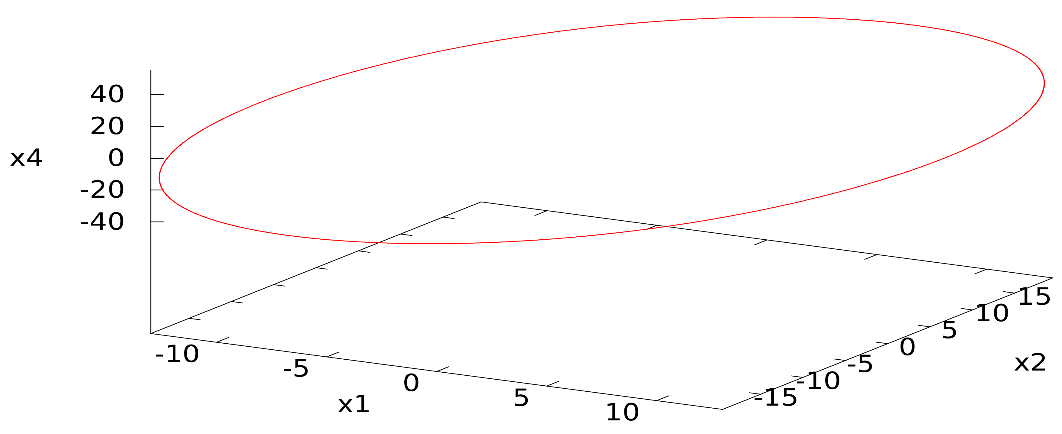
From this iterative procedure, we see that the limiting trajectory in this case is a cycle with a period $T_c\approx 0.3655$. Its projections are shown in Figure 1 and Figure 2.

To select the value $\Delta t_P$, this step must be reduced until the rapprochement distance $d_{k^{*}}$ changes significantly.

This approach is also applied for other initial conditions. As a result, we obtain the same cycle.

Next, we investigate the stability of the resulting cycle by calculating the Lyapunov exponents.

6. Calculation of the Lyapunov Exponents

In [20], a modification of the algorithm for calculating the Lyapunov exponents for a model describing the growth of a cancerous tumor was considered. Next, we consider a generalization of this algorithm for dynamical systems with a quadratic right-hand side of the n-th order. Note that another algorithm for calculating the Lyapunov exponents based on calculating the fundamental matrix of the dynamical system and its QR decomposition is proposed in [29]. The procedure described below can also be applied to it.

First, we define the form of the linearized system of equations. Let us denote the perturbations by the following:

$$x_{n+1}\left(t\right),x_{n+2}\left(t\right),\dots ,x_{2n}\left(t\right).$$

We define the form of the following expression using the rule for differentiating the sums and products:

$$\begin{array}{c}{\displaystyle \frac{\partial \langle Q_{p}X,X\rangle }{\partial x_j}}·x_{n+j}={\displaystyle \frac{\partial }{\partial x_j}}\left({\displaystyle \sum _{i=1}^n\sum _{k=1}^n{q}_{i,k}^{\left(p\right)}{x}_i{x}_k}\right)·x_{n+j}=\\ {\displaystyle =\left({\displaystyle \sum _{k=1}^n{q}_{j,k}^{\left(p\right)}{x}_k+\sum _{i=1}^n{q}_{i,j}^{\left(p\right)}{x}_i}\right)·x_{n+j}=\sum _{i=1}^n\left(q_{i,j}^{\left(p\right)}+q_{j,i}^{\left(p\right)}\right)x_i{x}_{n+j},}\end{array}$$

where $p=\overline{1;n}$, $j=\overline{1;n}$. Let us find the product as follows:

$$\begin{array}{c}\left[{\displaystyle \frac{\partial \langle Q_{p}X,X\rangle }{\partial x_1}}{\displaystyle \frac{\partial \langle Q_{p}X,X\rangle }{\partial x_2}}\dots {\displaystyle \frac{\partial \langle Q_{p}X,X\rangle }{\partial x_n}}\right]·\left[\begin{array}{c}{x}_{n+1}\\ x_{n+2}\\ ⋮\\ x_{2n}\end{array}\right]=\\ {\displaystyle =\sum _{j=1}^n\sum _{i=1}^n\left(q_{i,j}^{\left(p\right)}+q_{j,i}^{\left(p\right)}\right)x_i{x}_{n+j}=\sum _{i=1}^n\sum _{j=n+1}^{2n}\left(q_{i,j-n}^{\left(p\right)}+q_{j-n,i}^{\left(p\right)}\right)x_i{x}_j.}\end{array}$$

(11)

Next, we extend the system (1) by adding to it a linearized system, which also has a quadratic right-hand side. To do this, we introduce the extended matrix $\tilde{A}$:

$$\tilde{A}={\left[{\tilde{a}}_{i,j}\right]}_{2n\times 2n},{\tilde{a}}_{i,j}=\left\{\begin{array}{c}{a}_{i,j},\mathrm{if}i=\overline{1;n}\&j=\overline{1;n},\hfill \\ a_{i-n,j-n},\mathrm{if}i=\overline{n+1;2n}\&j=\overline{n+1;2n},\hfill \\ 0\mathrm{otherwise}.\hfill \end{array}\right.$$

The vector function $\tilde{X}\left(t\right)$ is equal to the following:

$$\tilde{X}\left(t\right)={\left[x_1\left(t\right)x_2\left(t\right)\dots x_n\left(t\right)x_{n+1}\left(t\right)\dots x_{2n}\left(t\right)\right]}^{\mathrm{T}}.$$

Based on Formula (11), we have a quadratic form on the right-hand side of the linearized system for each equation. Then, to reduce the system to a general form, we introduce the following extended matrix:

$$\begin{array}{c}{\tilde{Q}}_l={\left[{\tilde{q}}_{i,j}^{\left(l\right)}\right]}_{2n\times 2n},\hfill \\ \mathrm{for}l=\overline{1;n}:{\tilde{q}}_{i,j}^{\left(l\right)}=\left\{\begin{array}{c}{q}_{i,j}^{\left(l\right)},\mathrm{if}i=\overline{1;n}\&j=\overline{1;n},\hfill \\ 0\mathrm{otherwise},\hfill \end{array}\right.\hfill \\ \mathrm{for}l=\overline{n+1;2n}:{\tilde{q}}_{i,j}^{\left(l\right)}=\left\{\begin{array}{c}{q}_{i,j-n}^{(l-n)}+q_{j-n,i}^{(l-n)},\mathrm{if}i=\overline{1;n}\&j=\overline{n+1;2n},\hfill \\ 0\mathrm{otherwise}.\hfill \end{array}\right.\hfill \end{array}$$

We get an extended system similar to the system (2):

$$\dot{\tilde{X}}=\tilde{A}\tilde{X}+\tilde{\mathsf{\Phi }}\left(\tilde{X}\right),$$

(12)

where

$$\begin{array}{c}\tilde{\mathsf{\Phi }}={\left[{\tilde{\phi }}_1\left(\tilde{X}\right)\dots {\tilde{\phi }}_{2n}\left(\tilde{X}\right)\right]}^{\mathrm{T}},\\ {\tilde{\phi }}_l\left(\tilde{X}\right)=\langle {\tilde{Q}}_l\tilde{X},\tilde{X}\rangle ,l=\overline{1;2n}.\end{array}$$

To obtain the domain of convergence of the power series that is a solution to the system (12), the norms of the matrices are calculated as follows:

$$\parallel \tilde{A}\parallel ,\parallel {\tilde{Q}}_1\parallel ,\parallel {\tilde{Q}}_2\parallel ,\dots \parallel {\tilde{Q}}_{2n}\parallel$$

and the number

$$\tilde{\mu }=2n\underset{p=\overline{1;2n}}{max}\parallel {\tilde{Q}}_p\parallel .$$

Let

$$\tilde{X}\left(t\right)=\sum _{i=0}^{\infty }{\tilde{\mathrm{Y}}}_i{t}^i,$$

(13)

where ${\tilde{\mathrm{Y}}}_0=\tilde{X}\left(0\right)$ is the initial condition for the system (12),

$${\tilde{\mathsf{\Psi }}}_i={\left[{\tilde{\psi }}_{i,1}\dots {\tilde{\psi }}_{i,2n}\right]}^{\mathrm{T}}$$

and

$${\tilde{\psi }}_{i,p}=\sum _{j=0}^i\langle {\tilde{Q}}_p{\tilde{\mathrm{Y}}}_j,{\tilde{\mathrm{Y}}}_{i-j}\rangle ,p=\overline{1;2n}.$$

By analogy with the system (2), two auxiliary numbers are calculated as functions of ${\tilde{\mathrm{Y}}}_0$:

$$\begin{array}{c}{\tilde{h}}_1\left({\tilde{\mathrm{Y}}}_0\right)=\parallel {\tilde{\mathrm{Y}}}_0\parallel ,\\ {\tilde{h}}_2\left({\tilde{\mathrm{Y}}}_0\right)=\left\{\begin{array}{c}\tilde{\mu }{\tilde{h}}_1^2\left({\tilde{\mathrm{Y}}}_0\right)+(\parallel \tilde{A}\parallel +2\tilde{\mu }){\tilde{h}}_1\left({\tilde{\mathrm{Y}}}_0\right),\mathrm{if}{\tilde{h}}_1>1,\hfill \\ \parallel \tilde{A}\parallel +\tilde{\mu }\mathrm{otherwise}.\hfill \end{array}\right.\end{array}$$

Then, the power series (13) converges for $t\in [-\tilde{\tau },\tilde{\tau }]$, where the following holds:

$$\tilde{\tau }=\tilde{\tau }\left({\tilde{\mathrm{Y}}}_0\right)={\displaystyle \frac{1}{{\tilde{h}}_2\left({\tilde{\mathrm{Y}}}_0\right)+\delta }},$$

and $\delta$ is any positive number.

Let us consider a modification of Benettin’s algorithm for calculating the Lyapunov exponents using the Gram–Schmidt orthogonalization [10] (pp. 163–165):

• Divide a given time interval $[0,T]$ (usually the value T is large) into short intervals by the following length:

  $${\tau }_M={\displaystyle \frac{T}{M}},$$

  where M is the number of such intervals.
• Let$X^{*}$ be a point of the researched solution, e.g., (10);
• $k:=0$;
• $Y^{\left(k\right)}:=X^{*}$;
• Let$Z_{\left(p\right)}^{\left(k\right)}$ be the column vectors of initial perturbations from n-components (the real numbers), $p=\overline{1;n}$ (p is a number of the perturbation vector);
• Assign to each component of the vector $Z_{\left(p\right)}^{\left(k\right)}$ random number in the range $[0,1]$;
• $L{E}_p:=0$, $p=\overline{1;n}$ (the initial values of the sums at calculating the Lyapunov exponents);
• Orthogonalize and normalize to unity the system of vectors $Z_{\left(1\right)}^{\left(k\right)}$, $Z_{\left(2\right)}^{\left(k\right)}$,..., $Z_{\left(n\right)}^{\left(k\right)}$;
• $k:=k+1$;
• Forp from 1 to n with step 1:
  Beginning of cycle
  Let

  $$\tilde{X}\left(0\right):=\left[\begin{array}{c}\hfill Y^{(k-1)}\\ \hfill Z_{\left(p\right)}^{(k-1)}\end{array}\right].$$
  Find$\tilde{X}\left({\tau }_M\right)$ for the system (12) on the algorithm, described in Section 4.
  Assign to vectors $Y^{\left(k\right)}$ and $Z_{\left(p\right)}^{\left(k\right)}$ the matching vector blocks $\tilde{X}\left({\tau }_M\right)$, i.e.,

  $$\left[\begin{array}{c}\hfill Y^{\left(k\right)}\\ \hfill Z_{\left(p\right)}^{\left(k\right)}\end{array}\right]:=\tilde{X}\left({\tau }_M\right).$$
  Note that for all values of p the vector $Y^{\left(k\right)}$, is the same.
  End of cycle
• Forp from 1 to n with step 1:
  Beginning of cycle
  ${\displaystyle S:=Z_{\left(p\right)}^{\left(k\right)}-\sum _{i=1}^{p-1}〈Z_{\left(p\right)}^{\left(k\right)},Z_{\left(i\right)}^{\left(k\right)}〉·Z_{\left(i\right)}^{\left(k\right)};}$
  $L{E}_p:=L{E}_p+log\left|S\right|;$
  $Z_{\left(p\right)}^{\left(k\right)}:={\displaystyle \frac{S}{\left|S\right|}}.$
  End of cycle
• If$k<M$, then Go to step 9;
• $L{E}_p:={\displaystyle \frac{L{E}_p}{M·{\tau }_M}}$, $p=\overline{1;n}$;
• Print$L{E}_p$, $p=\overline{1;n}$.

For the point (10), the Lyapunov exponents were found using the described algorithm for $T=100$, $M=$ 20,000 and ${\tau }_M=0.005$. Next, we give them the following approximate values:

$$L{E}_1\approx 0,L{E}_2\approx -0.498,L{E}_3\approx -0.499,L{E}_4\approx -20.002.$$

As can be seen, their signature corresponds to a stable limit cycle in the system (1), which confirms the presence of the cycle, found through the study of the Poincaré recurrences. Note that in [30] an alternative numerical–analytical scheme for constructing periodic solutions of systems with a quadratic right-hand side was proposed using an example of the Lorenz system. Now, this scheme is being actively developed in [31,32,33] to find periodic solutions of nonlinear systems of differential equations.

The graphs of changes in the Lyapunov exponents over time are shown in Figure 3, Figure 4, Figure 5 and Figure 6.

7. Conclusions

In this article, the author investigates the limiting regimes corresponding to different initial points of the phase space. As a result, we obtain the same cycle shown in Figure 1 and Figure 2. Consequently, there is no hyperchaos in system (1).

The analysis of the Poincaré recurrences, described in the goals of research, showed that the rapprochement with the initial point occurs approximately at the same time (i.e., we have a regularity). This indicates a limit cycle in system (1).

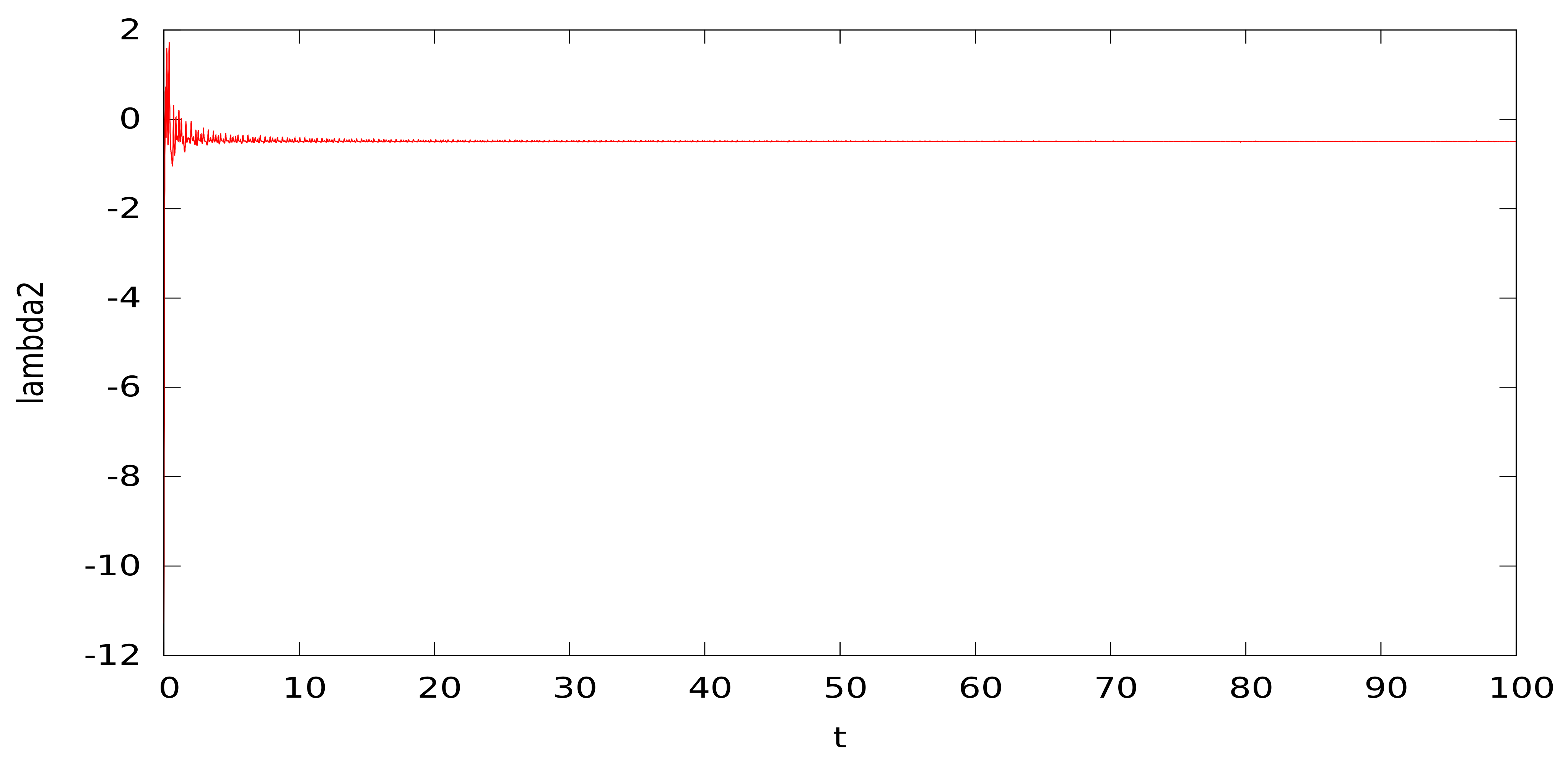
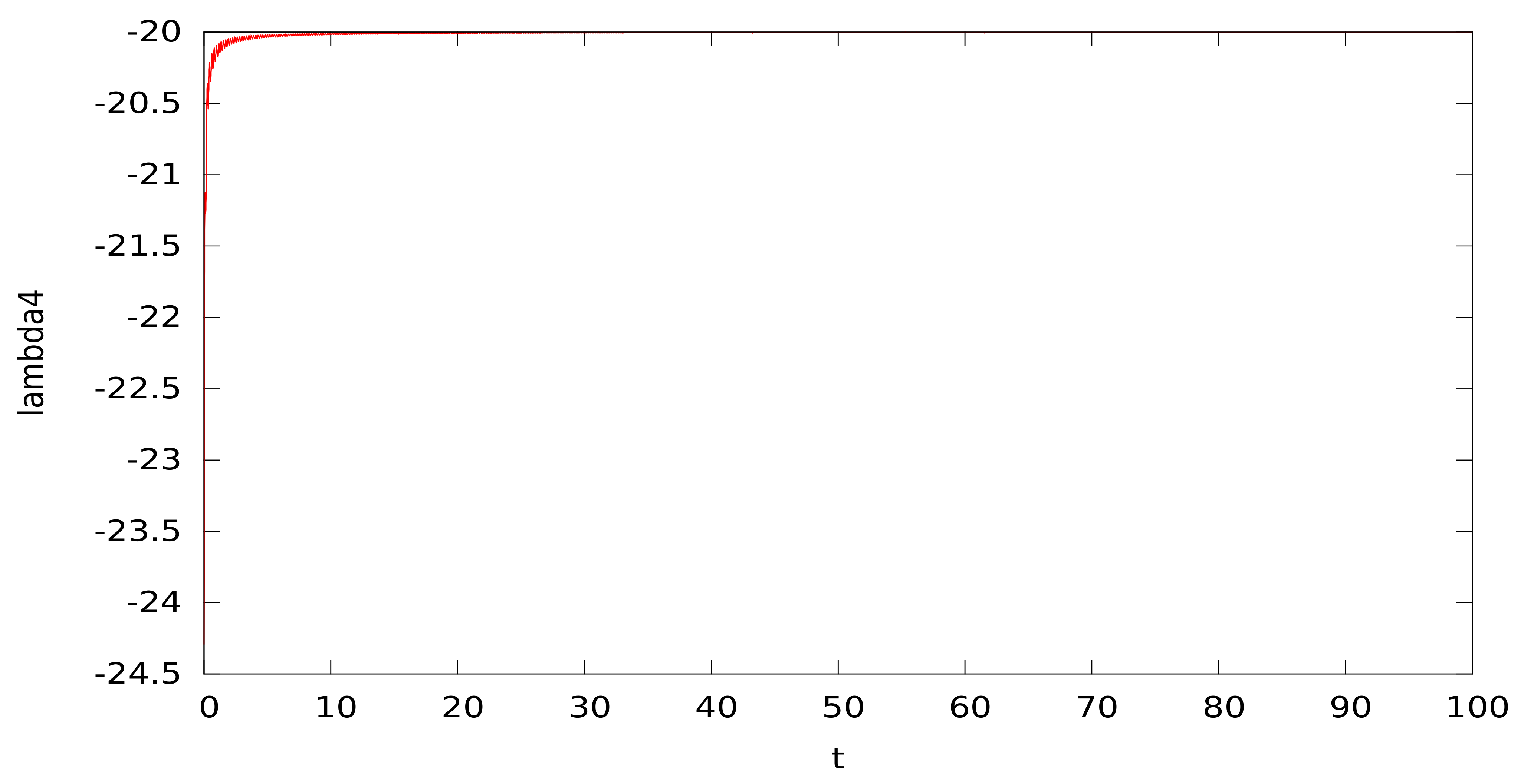
Stabilization of the behavior of the values of the Lyapunov exponents in Figure 3, Figure 4, Figure 5 and Figure 6 indicates the correctness of finding their limiting values over a relatively short time interval $[0,100]$.

Thus, the limiting trajectory investigated using the analysis of the Poincaré recurrences and the high-precision calculation of the Lyapunov exponents (i.e., different methods) is the limit cycle, which contradicts the results in [22] for the values of the parameters $a=7$, $b=50$, $c=3$, $d=10$, $e=5$, $f=5$ and $k=1.5$ of system (1). The obtained data are available at [34]. Most likely, the authors of the article [22] made a typo indicating such values of the parameters at which they found a hyperchaos.

A significant novelty of the article is the high-precision method for searching for the Poincaré recurrences on attractors of dynamical systems with a quadratic right-hand side, as well as a modification of Benettin’s algorithm for finding the Lyapunov exponents in order to check the found limiting regimes.

The methods described in the article can be used to study not only periodic regimes, but also quasiperiodic and chaotic regimes for dynamical systems with a quadratic right-hand side. According to the statistics of Poincaré recurrences, we can determine the dimension of the attractor and compare it with the dimension obtained when calculating the Lyapunov exponents (for example, the articles [17,18]).

The advantage of the considered algorithm for calculating the Lyapunov exponents is the combination of the linearized system of equations and the original dynamical system in a general form (12) for finding the state and perturbation vectors together.

References

- Sprott, J.C. Elegant Chaos: Algebraically Simple Chaotic Flows; World Scientific Publishing: Singapore, 2010; p. 304. [Google Scholar] [CrossRef]
- Tancredi, G.; Sánchez, A.; Roig, F. A comparison between methods to compute Lyapunov exponents. Astron. J. 2001, 121, 1171–1179. [Google Scholar] [CrossRef]
- Lozi, R.; Pchelintsev, A.N. A new reliable numerical method for computing chaotic solutions of dynamical systems: The Chen attractor case. Int. J. Bifurc. Chaos 2015, 25, 1550187. [Google Scholar] [CrossRef] [Green Version]
- Lozi, R.; Pogonin, V.A.; Pchelintsev, A.N. A new accurate numerical method of approximation of chaotic solutions of dynamical model equations with quadratic nonlinearities. Chaos Solitons Fractals 2016, 91, 108–114. [Google Scholar] [CrossRef] [Green Version]
- Jafari, S.; Sprott, J.C.; Nazarimehr, F. Recent new examples of hidden attractors. Eur. Phys. J. Spec. Top. 2015, 224, 1469–1476. [Google Scholar] [CrossRef]
- Nemytskii, V.V.; Stepanov, V.V. Qualitative Theory of Differential Equations; Dover Publications: New York, NY, USA, 1989; p. 523. [Google Scholar]
- Afanas’ev, A.P.; Dzyuba, S.M. Method for constructing minimal sets of dynamical systems. Differ. Equ. 2015, 51, 831–837. [Google Scholar] [CrossRef]
- Afanas’ev, A.P.; Dzyuba, S.M. Construction of the minimal sets of differential equations with polynomial right-hand side. Differ. Equ. 2015, 51, 1403–1412. [Google Scholar] [CrossRef]
- Afanas’ev, A.P.; Dzyuba, S.M. On recurrent trajectories, minimal sets, and quasiperiodic motions of dynamical systems. Differ. Equ. 2005, 41, 1544–1549. [Google Scholar] [CrossRef]
- Kuznetsov, S.P. Dynamical Chaos, 2nd ed.; Fizmatlit: Moscow, Russia, 2006; p. 356. (In Russian) [Google Scholar]
- Afraimovich, V.; Lin, W.; Rulkov, N. Fractal dimension for Poincaré recurrences as an indicator of synchronized chaotic regimes. Int. J. Bifurc. Chaos 2000, 10, 2323–2337. [Google Scholar] [CrossRef]
- Afraimovich, V.; Zaslavsky, G.M. Fractal and multifractal properties of exit times and Poincaré recurrences. Phys. Rev. E 1997, 55, 5418–5426. [Google Scholar] [CrossRef]
- Kac, M.; Uhlenbeck, G.E.; Hibbs, A.R.; Pol, B.V.D.; Gillis, J. Probability and Related Topics in Physical Sciences; Interscience: New York, NY, USA, 1959; p. 266. [Google Scholar]
- Penné, V.; Saussol, B.; Vaienti, S. Fractal and statistical characteristics of recurrence times. Int. Conf. Disord. Chaos Honour Giovanni Paladin 1998, 8, 163–171. [Google Scholar] [CrossRef]
- Afraimovich, V.; Ugalde, E.; Urias, J. Fractal Dimensions for Poincaré Recurrences; Elsevier: Amsterdam, The Netherlands, 2006; Volume 2, p. 258. [Google Scholar]
- Anishchenko, V.S.; Khairulin, M.; Strelkova, G.; Kurths, J. Statistical characteristics of the Poincaré return times for a one-dimensional nonhyperbolic map. Eur. Phys. J. B 2011, 82, 219–225. [Google Scholar] [CrossRef]
- Anishchenko, V.S.; Birukova, N.I.; Astakhov, S.V.; Boev, S.V. Poincaré recurrences time and local dimension of chaotic attractors. Russ. J. Nonlinear Dyn. 2012, 8, 449–460. (In Russian) [Google Scholar] [CrossRef]
- Anishchenko, V.S.; Boev, Y.I.; Semenova, N.I.; Strelkova, G.I. Local and global approaches to the problem of Poincaré recurrences. Applications in nonlinear dynamics. Phys. Rep. 2015, 587, 1–39. [Google Scholar] [CrossRef]
- Guedes, P.F.S.; Nepomuceno, E.G. Some remarks on the performance of Matlab, Python and Octave in simulating dynamical systems. Anais do 14° SBAI 2019, 1, 554–560. [Google Scholar] [CrossRef]
- Pchelintsev, A.N. An accurate numerical method and algorithm for constructing solutions of chaotic systems. J. Appl. Nonlinear Dyn. 2020, 9, 207–221. [Google Scholar] [CrossRef]
- Babadzhanjanz, L.K.; Sarkissian, D.R. Taylor series method for dynamic systems with control: Convergence and error estimates. J. Math. Sci. 2006, 139, 7025–7046. [Google Scholar] [CrossRef]
- Dong, E.; Zhang, Z.; Yuan, M.; Ji, Y.; Zhou, X.; Wang, Z. Ultimate boundary estimation and topological horseshoe analysis on a parallel 4D hyperchaotic system with any number of attractors and its multi-scroll. Nonlinear Dyn. 2019, 95, 3219–3236. [Google Scholar] [CrossRef]
- Demidovich, B.P. Lectures on Mathematical Theory of Stability; Nauka: Moscow, Russia, 1967; p. 472. (In Russian) [Google Scholar]
- Pchelintsev, A.N. Numerical and physical modeling of the dynamics of the Lorenz system. Numer. Anal. Appl. 2014, 7, 159–167. [Google Scholar] [CrossRef]
- Pchelintsev, A.N.; Ahmad, S. Solution of the Duffing equation by the power series method. Trans. TSTU 2020, 26, 118–123. [Google Scholar] [CrossRef]
- Overton, M.L. Numerical Computing with IEEE Floating Point Arithmetic; SIAM: Philadelphia, PA, USA, 2001; p. 106. [Google Scholar] [CrossRef]
- GNU MPFR Library for Multiple-Precision Floating Point Computations with Correct Rounding. Available online: http://www.mpfr.org (accessed on 18 July 2021).
- Fousse, L.; Hanrot, G.; Lefèvre, V.; Pélissier, P.; Zimmermann, P. MPFR: A multiple-precision binary floating-point library with correct rounding. ACM Trans. Math. Softw. 2007, 33, 13. [Google Scholar] [CrossRef]
- Kuznetsov, N.V.; Leonov, G.A.; Mokaev, T.N.; Prasad, A.; Shrimali, M.D. Finite-time Lyapunov dimension and hidden attractor of the Rabinovich system. Nonlinear Dyn. 2018, 92, 267–285. [Google Scholar] [CrossRef] [Green Version]
- Pchelintsev, A.N. A numerical-analytical method for constructing periodic solutions of the Lorenz system. Differ. Uravn. i Protsesy Upr. 2020, 4, 59–75. [Google Scholar]
- Luo, A.C.J.; Huang, J. Approximate solutions of periodic motions in nonlinear systems via a generalized harmonic balance. J. Vib. Control 2011, 18, 1661–1674. [Google Scholar] [CrossRef]
- Luo, A.C.J. Toward Analytical Chaos in Nonlinear Systems; John Wiley & Sons: Chichester, UK, 2014; p. 258. [Google Scholar]
- Luo, A.C.J.; Guo, S. Analytical solutions of period-1 to period-2 motions in a periodically diffused brusselator. J. Comput. Nonlinear Dyn. 2018, 13, 090912. [Google Scholar] [CrossRef]
- Pchelintsev, A. The Reliable Calculations for the 4-th Order System. GitHub. Available online: https://github.com/alpchelintsev/4th_order_system (accessed on 18 July 2021).
Figure 1.
Projection of the cycle of the system (1) with the period into the space .
Figure 2.
Figure 3.
The graph of the change in time of the Lyapunov exponent .
Figure 4.
Figure 5.
Figure 6.