
Synthetic Data Augmentation and Deep Learning for the Fault Diagnosis of Rotating Machines


Department of Mechanical, Robotics and Energy Engineering, Dongguk University-Seoul, 30 Pil-dong 1 gil, Jung-gu, Seoul 04620, Korea
*
Author to whom correspondence should be addressed.
Mathematics 2021, 9(18), 2336; https://0-doi-org.brum.beds.ac.uk/10.3390/math9182336
Submission received: 1 September 2021
/
Revised: 17 September 2021
/
Accepted: 17 September 2021
/
Published: 21 September 2021
(This article belongs to the Special Issue Deep Learning and Machine Learning Mathematical Models for Computer Assisted Diagnostic Systems)
Abstract
:As failures in rotating machines can have serious implications, the timely detection and diagnosis of faults in these machines is imperative for their smooth and safe operation. Although deep learning offers the advantage of autonomously learning the fault characteristics from the data, the data scarcity from different health states often limits its applicability to only binary classification (healthy or faulty). This work proposes synthetic data augmentation through virtual sensors for the deep learning-based fault diagnosis of a rotating machine with 42 different classes. The original and augmented data were processed in a transfer learning framework and through a deep learning model from scratch. The two-dimensional visualization of the feature space from the original and augmented data showed that the latter’s data clusters are more distinct than the former’s. The proposed data augmentation showed a 6–15% improvement in training accuracy, a 44–49% improvement in validation accuracy, an 86–98% decline in training loss, and a 91–98% decline in validation loss. The improved generalization through data augmentation was verified by a 39–58% improvement in the test accuracy.
1. Introduction
Rotating machines are the backbone of a variety of modern applications, such as power turbines, pumps, automobiles, and oil/gas refineries [1,2,3,4,5]. These machines are vulnerable to unavoidable malfunction during their operation due to load fluctuations, and material degradation with time. The unexpected failures of rotating machines may result in substantial economic losses associated with maintenance costs and production halts, as well as personnel casualties due to catastrophic failure. Commonly encountered defects in rotating machines are unbalance, misalignment, rubbing, cracks in the shafts, bearing faults, and gearbox fault [6,7]. For efficient maintenance strategies and the safe operation of rotating machines, it is imperative to detect, isolate, and quantify different defects in these machines in a timely manner.
In the last decade, artificial intelligence (machine learning, deep learning) has been extensively applied for the fault diagnosis and prognosis of rotating machines. State of the art reviews of the use of machine learning and deep learning for the fault diagnosis of rotating machines can be found in recent articles [4,8,9]. Kolar et al. [10] proposed a fault diagnosis strategy for rotary machinery using a convolutional neural network (CNN); the vibration signals of a three-axis accelerometer were supplied as high-definition images to the CNN, which automatically extracted the discriminative features, and classified the input data into four classes: normal, unbalance, cracked rotor, and bearing fault. Qian et al. [11] proposed a transfer learning method called improved joint distribution adaptation (IJDA) for the fault diagnosis of the bearing and the gearbox under variable working conditions. Janssens et al. [12] studied a convolutional neural network for the autonomous feature learning of bearing faults, lubrication degradation, and rotor imbalance; their comparison between the autonomous feature learning through CNN and conventional handcrafted feature engineering showed that, in terms of accuracy, the former outperformed the later by 7.29%. Martinez-Rego et al. [13] employed one-class support vector machines (SVM) for the fault detection of a power windmill while using only the normal condition data during the training phase; the proposed method was able to identify the presence and evolution of defect in the datasets from simulation, controlled experiment, and the real windmill power machine. Li et al. [14] proposed least square mapping and fuzzy neural network for the condition diagnosis of rotating machinery, and verified the method for the outer-race defect, inner-race defect, and roller defect in rolling bearings. Umbrajkaar et al. [15] proposed the combination of artificial neural network and support vector machine for the assessment of parallel and angular misalignment under variable load condition. Yan et al. [16] studied the unbalance fault in rotor using deep belief network (DBN), and the fusion of multisource heterogeneous information.
In recent years, data-driven approaches have been extensively studied for the efficient and robust fault diagnosis of rotating machines [4,17]. Depending on the size of data, data-driven techniques are employed either for fault diagnosis strategies machine learning, or deep learning. In the general framework of machine learning, the commonly employed processing steps are: the obtaining of sensor data in healthy and faulty states → preprocessing → discriminative feature extraction → feature selection → training/validation → testing of the pretrained model → deployment of the pretrained model for fault diagnosis [18,19], whereas, in the general framework of deep learning, the common processing steps are: sensor data in healthy and faulty states → preprocessing → autonomous feature extraction + training & validation → testing of the pretrained model → deployment of the pretrained model for fault diagnosis [20,21,22]. Although traditional machine learning algorithms are efficient for fault diagnosis from limited data, the process of feature engineering is labor-intensive, time-consuming, and requires sufficient domain knowledge and diagnostic skills. On the other hand, although deep learning eliminates the need for human engineered discriminative features, a substantial amount of healthy and faulty data is required to autonomously identify those features from the data. In practice, there exists an issue of data imbalance where there is sufficient data from the healthy state, while very limited data is available from the faulty states of the system. Contrary to the stochastic machine learning and deep learning models, deterministic artificial intelligence (DAI) takes into account the first principles (i.e., underlying physics of the problem) whenever available [23,24].
To minimize economic loss and downtime by improving operational efficiency at industrial facilities, a fault diagnosis of the industrial assets is actively carried out. For the last decade, continuous research efforts have been made to replace the human expert-based fault diagnostic procedures with artificial intelligence (AI)-based diagnostic methods. Whereas in the former, the diagnosis procedure is heavily dependent on the diagnostic expertise of a human expert, in the latter, the condition of an industrial facility is assessed by processing the sensor data in real-time. While human experts have limitations in assessing large amounts of data, recent advancements in hardware and software have allowed AI-based methods to efficiently process large data for diagnostic purposes. Although deep learning-based diagnostic procedures automatically extract the discriminative features of different health states, the requirement of sufficient data from those health states impedes their applicability. In general practice, while sufficient healthy state data is available, it is very difficult to obtain faulty state data because, upon suspicion of a fault or failure, the system is immediately shut down. The data imbalance between different health states usually results in a biased system [25], where the probability of optimally identifying different health states drops significantly. The data imbalance usually restricts the application of deep learning models to only binary classification, i.e., healthy or faulty.
One way to cope with the issue of data scarcity from healthy and faulty states is synthetic data augmentation, where new samples are generated from the original data through different techniques [26]. The process of data augmentation helps to improve the generalizability and robustness of deep learning-based diagnostic strategies [27]. For real-world image classification via deep learning, commonly used data augmentation techniques include random cropping, different levels of rotations, adding Gaussian noise, and contrast variations [28,29,30]. For time series data, commonly employed augmentation techniques include cropping or slicing, widowing, the ensemble-based method, generative adversarial networks (GANs), and the addition of Gaussian noise [31,32,33,34,35]. Fu and Wang [36] proposed the combination of generative adversarial network (GAN) and stacked denoising auto-encoder (SDAE) for deep learning-based data augmentation and the fault diagnosis of bearings and gears. Li et al. [37] investigated the sample-based and dataset-based augmentation methods using the augmentation techniques of adding Gaussian noise, masking noise, signal translation, amplitude shifting, and time stretching for bearing fault diagnosis. Hu et al. [38] proposed a resampling technique based on order tracking for data augmentation and self-adaptive CNN for fault diagnosis from limited faulty states data. Kamycki et al. [39] proposed a synthetic data augmentation technique for time series classification using suboptimal warping. Liu et al. [40] proposed the four methods of adding noise, permutation, scaling, and warping for time series data augmentation, and verified these methods using a fully connected neural network and the pretrained model of ResNet.
The current work proposes the augmentation of data through virtual sensors to provide deep learning models with additional information for the efficient detection, isolation, and quantification of different faults in rotating machines. Virtual sensors are defined in terms of actual proximity probes through the principle of coordinate transformation. The original and augmented datasets are transformed into scalograms, and processed through the pretrained deep learning models of ResNet18 [41] and SqueezeNet [42] in a transfer learning framework, as well as through a deep learning model from scratch. The results of the original and augmented data are compared in terms of training accuracy, validation accuracy, training loss, validation loss, test accuracy, and the test confusion matrix. The effect of the number of virtual sensors on the learning behavior of the deep learning models is demonstrated by considering data augmentation through 8 and 16 virtual sensors. Furthermore, the effectiveness of data augmentation for fault diagnosis is shown by depicting the feature space of the original and augmented data set on a two-dimensional plot through principal component analysis (PCA) [43], and t-distributed stochastic neighbor embedding (t-SNE) [44]. The proposed approach would help in solving the issue of data imbalance between the healthy and faulty datasets, as well as synthetically augmenting limited experimental data for deep learning-based fault diagnosis.
2. Proposed Methodology
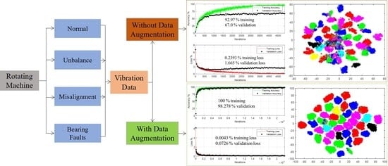
This section describes the proposed methodology of the fault detection, isolation, and quantification using synthetic data augmentation and deep learning algorithms. Figure 1 shows a schematic of the overall process.
In this process, several defects are simulated using Spectra-Quest’s Machinery Fault Simulator (SpectraQuest Inc., Richmond, VA, USA), and vibration data is obtained for each defect. The time-domain vibration responses are obtained through several sensors, and are transformed into scalograms in the original form, as well as after augmentation through virtual sensors. The details of synthetic data augmentation are discussed in Section 2.2. The vibration scalograms of the original and augmented data are processed in two ways: to train a customized deep learning model from scratch, and to employ transfer learning using existing pretrained deep learning models. Finally, the results of the original and augmented datasets are compared in terms of the training, validation, and testing accuracies of the deep learning models. The following sections provide details of each stage of the proposed methodology.
2.1. Description of Dataset
To evaluate the contributions of the current work and validate the proposed methodology, a comprehensive dataset, named as machinery fault data base (MaFaulDa) [45], is selected. The chosen dataset is extensive enough and includes multiple faults in the rotor system and in the supporting bearings, with each fault at different severity levels and different speeds of operation. The SpectraQuest’s machinery fault simulator (MFS) alignment–balance–vibration trainer (ABVT) [46] was used to obtain the MaFaulDa in the form of a multivariate time series. Figure 2 shows the experimental setup to emulate the dynamics of mass unbalance, horizontal misalignment, vertical misalignment, and bearing faults.
In this setup, the speed of rotation is measured by a tachometer. The axial, radial, and tangential accelerations are measured with two distinct sets of accelerometers, one at each bearing. The operational sound of the system is measured with a microphone. The eight sensors are used to acquire the healthy and faulty states data for 5 s at a rate of 50 kHz. Table 1 summarizes the types of health states, their severity levels, and speeds of operation.
In Table 1, three different bearings with outer race fault, rolling element fault, and inner race fault were placed one at a time at two different positions: the underhung position (i.e., defective bearing between the rotor and motor), and the overhung position (i.e., having the rotor between the defective bearing and motor). Furthermore, the bearing faults were simulated in the presence of 0, 6, 20, and 35 g unbalances to make the imperceptible faults more pronounced. The measurements from all the health states resulted in a 1951 × 8 multivariate time series, where 1951 is the number of different measurement scenarios, and 8 is the number of sensor signals for each scenario. The size of the database is 13 gigabytes and is available for download at the website [44].
Several authors have used the MafaulDa database for the validation of their proposed methodology and proof of concept. Table 2 summarizes the previously performed research using the same dataset as selected by the authors in the current work.
Although the MaFaulDa dataset is comprised of 42 different classes of various severity levels (Table 1), the published literature on the dataset either studied the health states in general, without any consideration of the severity of each health state, or only studied a subset of the entire dataset. The objective of the current work is to demonstrate the effectiveness of synthetic data augmentation through virtual sensors for the fault diagnosis of rotating machines, by exploring the MaFaulDa dataset with all the health states, as well as the associated severity levels and the various speed of rotations of each health state.
2.2. Synthetic Data Augmentation
To solve the issue of data imbalance, this paper employs the idea of virtual sensors to artificially augment the vibration data of different health states, and automatically learn the characteristics of different faults through deep learning. The concept of virtual sensors is based on the idea of looking at the same point in space from different perspectives, using different coordinate systems, as shown in Figure 3.
In this, the same point P can have two different representations: P (x0, y0) on the X0, Y0 axes, and P (x1, y1) on the X1, Y1 axes, where the latter is obtained from the former through orientation at the origin by an angle of θ. The mathematical relation between the two coordinates for point P is expressed as follows:
Point P can be viewed in several different coordinates depending on the number of coordinate axes obtained from the base coordinate (X0, Y0) through orientation at the origin. The same principle can be extended to several scalar values in the time domain, such as a discrete vibration signal to look at that signal from different perspectives.
In this work, the principle of coordinate transformation is employed to augment the vibration signals that are obtained through two proximity sensors that were installed at right angles, as shown in Figure 4.
In this, due to symmetry around the centerline, the virtual vibration signals within the π rotation angle can be effective for synthetic data augmentation through virtual sensors. The virtual vibration signals are obtained from the actual vibration signals of the proximity probes using the coordinate transformation, as follows:
where, the subscripts V and A refer to the virtual and actual signals, respectively. The term ∆θ is the incremental angle of rotation between the actual and virtual sensors, and M = π/∆θ is the maximum number of virtual sensors that could be obtained from the actual signals. Wherein, due to the symmetry of the vibration signal around the centerline of the shaft, a maximum range for the incremental angle is 0–π. For a robust diagnostic strategy, the value of the incremental angle should be carefully chosen. A smaller value of the incremental angle may result in too many virtual signals and the subsequent increase in the computational cost of the classification algorithm. In addition, the smaller incremental angle can lead to redundant data that may adversely affect the classification performance. On the other hand, a larger value of the incremental angle will result in only a few virtual signals that may not provide sufficient additional information for improving the classification performance through virtual sensors. Moreover, because xVm is equal to yVm+N/2, only xVm was retained for data augmentation to avoid data duplication. The current work studies the effect of the incremental angle on the classification performance by comparing the results of larger and smaller incremental angles, as shown in Section 5. A more detailed discussion, and the validation of virtual signals, can be found in [53].
2.3. Scalograms of Vibration Signals
Figure 1 shows that the sensor data, with and without augmentation, were transformed into scalograms, which were processed with the deep learning models as image data. A scalogram contains the time–frequency information of a time series and is generated from the absolute values of the continuous wavelet transform (CWT) coefficient. The mathematical details on transforming a time domain signal into a scalogram can be found in the references [58,59,60]. For the current work, a CWT filter bank was precomputed in Matlab, and employed to transform the time domain signals into scalograms. For the current work, the Matlab 2020b was employed with the Wavelet Toolbox for wavelet coefficients of the signal, the Image Processing Toolbox for wavelet coefficient-to-image (i.e., scalogram) conversion and the resizing of the image, and the Deep Learning Toolbox for the implementation of customized deep learning models and transfer learning through pretrained deep learning models. The type of wavelet used in the filter bank was the analytic Morse wavelet (3,60), where 3 is the symmetry parameter, and 60 is the time–bandwidth product [61,62,63]. To gain an intuitive idea of the data augmentation through virtual sensors, Figure 5 compares the scalograms of some specific cases of normal, unbalance, and misalignment for the original signals and their augmented forms.
In this, the x and y axes of the scalograms refer to the time and frequency content of the signals, respectively. The y-axis of the scalograms is on log scale to account for the wide range of operating speeds, the presence of different levels of noise, and the different harmonics-associated defects. The horizontal line in all the scalograms (rectangular box) denotes the speed of rotation at a steady state. From the comparison of Figure 5a,b with Figure 5c,d, it is observed that, although when observed with the naked eye the virtual signals show slight variation from the original signal, these slight variations would provide the deep learning model with additional information on the original signals, as demonstrated in Section 4 and Section 5. The same is the case for the original and virtual signals of the unbalance and misalignment in Figure 5e–l.
3. Deep Learning Models
The vibration-based scalograms of the original and the augmented datasets are processed via two strategies of deep learning: transfer learning with preexisting deep learning models, and a customized deep learning model from scratch. The transfer learning strategies are employed to obtain baseline results by taking advantage of the architecture of the already available pretrained deep learning models developed by experts [64]. However, the fixed architecture and number of parameters of the pretrained deep learning models dilute their flexibility for problems of different types. The customized deep learning models could help to come up with deep learning models that are optimized in terms of architecture and the parameters for a specific problem.
In the current work, the pretrained models of ResNet18 [41] (He et al., 2016) and SqueezeNet [42] are adopted to obtain the baseline results from the original and augmented data using transfer learning. In transfer learning, the knowledge gained (e.g., weights, biases) from solving one problem is extended to solve another different, but related, problem [65]. For example, knowledge gained while learning to recognize real-world images (e.g., cars, trucks, birds, and flowers) could be extended to identify faults in the vibration-based images of mechanical systems [66,67]. In the general framework of transfer learning, a large amount of labelled data with different categories is used as source data to optimize the parameters of a deep learning model, and then tune/transfer those parameters to another related task with a small amount of target data.
In the general framework of transfer learning, all the layers of a well-trained network, except for the last layer, are transferred/copied to a new target task. The output layer of the well-trained deep learning model is modified according to the categories/classes of the target task, and the target data is used to tune the parameters of the network according to the new task. For mathematical elaboration, let the source (DSource) and target (DTarget) datasets be denoted, as shown by Equation (3):
where, X and L denote the input data and its labels, respectively, as provided to the network.
In terms of deep learning, the mapping of the input data to the output labels for the source and target datasets can be represented as follows:
where, DLM denotes a deep learning model with parameters θ that maps the input data (X) to the actual output labels (L) through the predicted labels .
In transfer learning, the mapping of the DLMSource is well-established by optimizing its parameters during the training process on the source task, as follows:
where, the term refers to the parameters of the deep learning model after training on the source data.
In transfer learning, the trained parameters of the first n layers of the DLMSource are transferred to the target task, as follows:
The other parameters of the DLMTarget are obtained during the training on the target data, as shown by Equation (7):
During the process of transfer learning, the parameters of the first n layers are fine-tuned with respect to the target training data using a small learning rate, while the parameters for the (n–m) layers θTarget (n:m) are trained from scratch on the target data. In general, the layers transferred from the source task to the target task are optimized for the detection and extraction of generic features and the input data, and are less sensitive to the variation of distribution of the inputs.
To explore the feasibility of a problem-specific neural network to be designed and trained from scratch, the original and augmented datasets were also processed with the customized deep learning model of Table 3.
Specific details on the function of each layer of the network are briefly described as follows:
Convolutional Layer: In the convolutional layers, a feature map is realized by applying a filter or kernel to the local regions of the input, shown by Figure 6.
The filter is an array of weight and biases which is multiplied with a patch of the image to obtain a weighted combination (scalar value) of that region of the input. The filter is applied multiple times to the input image and this results in a filtered image at the output, often referred to as the activations, or feature map, of that filter. There are as many filtered images at the output of a convolutional layer as the number of filters in that layer, and the filtered images are arranged in the form of three-dimensional array. The third dimension of the convolutional output is known as the number of channels. A typical example of output from the first convolutional layer of the deep learning model of Table 3 is shown in Figure 7.
Herein, it is observed that each filter is realizing different features of the input image, which are supplied to the next layers for further processing. The convolution process is mathematically described by Equation (8).
where, A is the output feature map of the filter, W and B, respectively, refer to the weights and bias of the filter, and L is the j-th local region. The subscript k and superscript i refer to the k-th filter in the i-th layer.
Batch Normalization: the batch normalization layer normalizes the input from the previous layer to mitigate the problem of the internal covariance shift, expediates the training process, and improves the accuracy of the model. During batch normalization, the output from the previous layer (the convolutional layer in this case) is first normalized by using the mean (μ) and standard deviation (σ) of the values, as shown by Equation (9).
Wherein, ε is a smoothing term to ensure numerical stability and avoid the division with a zero value. The learnable parameters of γ (gamma) and β (beta) are employed to rescale and offset the normalized values, as shown by Equation (10).
The optimum values for the parameters of γ (rescaling) and β (offsetting) are obtained during the training process.
Activation layer (ReLU): The activation layer enhances the representational ability of the deep learning network by adding nonlinearity to the output from the previous layer. In the literature, commonly adopted activation functions are linear, tanh, sigmoid, and the rectified linear unit (ReLU). In this work, the ReLU was employed as an activation function as it accelerates the convergence of the deep learning model. The ReLU is mathematically described as shown by Equation (11).
where Ac is the activation of the input yi. The ReLU returns a zero value if it receives a negative value and passes the positive value without any alteration, as shown in Figure 8.
Pooling Layer: The pooling layer reduces the spatial size of the feature space by downsampling the output from the previous layer with the aim of reducing the variance of the feature space and the number of parameters of the network. More specifically, the max-pooling layer reduces a subregion to its maximum, as shown in Figure 8.
Wherein, a max-pooling filter of the size 2 × 2 is moved two cells to the right and two cells downward (stride 2 × 2) to downsample the feature space.
Dropout Layer: The dropout layer [68], with a dropout probability in a range between 0–1, is added to ignore randomly chosen neurons during the training process. The aim of the dropout layer is to reduce the chances of overfitting by reducing the codependency of neurons during the training of the network.
The last global pooling layer is employed to reduce the number of parameters for the last fully connected layer by pooling the feature space. The classification layer with softmax function [69,70] is used to associate the feature space with 42 different classes. A more detailed discussion on the functions, and their related mathematical details, for different layers of the deep learning models can be found in [71,72,73].
4. Results on the Original Data
This section describes the results of transfer learning models (ResNet18, SqueezeNet) and a customized convolutional neural network using the scalograms of the original data from the rotor system of Figure 2.
4.1. Transfer Learning Results
The dataset of Table 1 is comprised of 1951 scenarios of 42 different classes, and each class is described in terms of eight signals obtained through the sensors. For the original dataset, without augmentation, all of the 15,608 (1951 × 8) time series were transformed directly into scalograms, without any preprocessing. The reason for considering the signals from all the sensors is to provide the deep learning model with sufficient data. The 15,608 scalograms of the original data were split into 80% training data, 10% validation data, and 10% test data. To leverage the knowledge of the pretrained networks and get a baseline accuracy on the original data, the deep learning models of ResNet18 and SqueezeNet were employed in a transfer learning framework. The reason for choosing two different pretrained models for transfer learning was to show the effect of the type of pretrained model. Figure 9 shows that the training and validation processes of the two models were interpreted in terms of accuracies and losses.
For transfer learning, both the networks were trained and validated for 50 epochs, with a learning rate of 0.001. In the training and validation plots of Figure 9, though the two models show an increasing trend in their training accuracy, and a decreasing trend in their training loss, their validation accuracy and validation loss do not follow the same trend. As the number of iterations/epochs increases, the difference between the training accuracy and validation accuracy also increases, and with the increasing number of epochs, the validation accuracy stops increasing further. A similar trend is observed for the training loss and validation loss, where with the increasing number of epochs, the validation loss stops decreasing further. The learning behavior of the deep learning models shown in Figure 9 is generally referred to as “Overfitting” [11,74,75] where, although the model fits the training data well, it cannot be generalized to new unseen instances of the problem at hand. Specifically, in the case of overfitting, the deep learning model learns/memorizes patterns that are more specific to the training data and cannot extend that pattern recognition capability to unseen data, thus hindering its reliable deployment for the health monitoring of an industrial asset. Moreover, while ResNet18 performs better than SqueezeNet in terms of training and validation accuracies, the validation loss of ResNet18 is larger than the validation loss of SqueezeNet. Furthermore, if looked at without the validation accuracy, the high training accuracy of ResNet18 could be misleading. Figure 10 and Figure 11 show the poor performance of an overfitted model on new unseen instances that can be observed from the confusion matrix of ResNet18 and SqueezeNet on the 10% test set.
In these, the rows and columns correspond to the labels of the true or actual classes, and the labels as predicted by the network for the given classes, respectively. The correctly and incorrectly classified observations are shown in cells on the diagonal and off-diagonal, respectively. The last column on the far right corresponds to the percentage of correctly classified observations for the actual or true classes, often referred to as the recall. The last row at the bottom shows the percentage of correctly classified observations of the predicted classes, commonly referred to as the precision. In general, the higher values of recall and precision reflect an optimally trained deep learning model. The test confusion matrix of Figure 10 shows that the deep learning model trained on the original dataset is confusing the observations of the same damage type (e.g., unbalanced of 6 g with unbalance of 10 g), as well as damage of different types (e.g., normal with unbalance, unbalance with misalignment, or bearing faults with misalignment).
More specifically, from the first row, out of the 39 observations for the normal case, 33 are correctly classified as normal, one as an unbalance with 6 g, one as a horizontal misalignment of 1.5 mm, one as a vertical misalignment of 1.27 mm, two as vertical misalignments of 1.9 mm, and one as a cage fault in the bearing at the underhung position. Similarly, from the second row, 23 out of 39 observations are correctly classified as unbalance of 6 g, one as normal, six as unbalance with 10 g, two as unbalance with 20 g, two as unbalance with 30 g, two as a horizontal misalignment of 0.5 mm, two as a vertical misalignment of 1.4 mm, and one as a cage fault in the bearing at the overhung position. The poor classification performance is also clearly observed from the low values of the recall and precision for different classes. Like the confusion matrix of ResNet18, the same interclass and intra-class confusion of different damage scenarios and different damage classes can be observed in the confusion matrix of SqueezeNet, as shown in Figure 11. Moreover, the relatively poor performance of SqueezeNet during the training process can be observed in Figure 11 from its relatively lower test classification accuracy of 60.95%.
To further explore the performance of a network that overfits the training data, t-distributed stochastic neighbor embedding (t-SNE) was employed to visualize the features from the last layer of ResNet18. In this work, principal component analysis (PCA) was used to reduce the dimensionality of the activations from the last pooling layer (i.e., pool 5) from 512 to 50, and the Barnes–Hut variant of the t-SNE algorithm [76] was used to visualize the distribution of different classes. Figure 12 shows a two-dimensional plot of the distribution of different classes.
In this, the overlap between the clusters of different classes reflects the poor performance and low classification accuracy of the deep learning model on the original data. Moreover, a model trained on the data with no clear distinction between different classes would not be able to generalize well to new unseen instances, as shown in the test confusion matrices of Figure 10.
4.2. Results from the Customized CNN
The dataset used in the transfer learning framework was also processed through the customized deep learning model of Table 3, and Figure 13 shows the training and validation process of the network.
The learning rate was kept at 0.001, and the network was trained for 50 epochs. From the training and validation performance of the network, it is that this network is performing relatively better than the transfer learning model of SqueezeNet. However, it has also overfitted the training data, and could not be generalized well to new unseen observations. The poor performance of the overfitted customized deep learning model on new observations could be verified from the test confusion matrix of Figure 14.
In this, the misclassified instances at the off-diagonal positions, and the lower values of recall and precision, confirm the poor performance of the overfitted network on new observations.
5. Results on Augmented Data
This section discusses the results of the transfer learning model of ResNet18 and customized CNN on the two scenarios of augmented data; a dataset augmented through eight virtual sensors, and a dataset augmented through 16 virtual sensors. The incremental angles for 8 and 16 virtual sensors were chosen to be (2k + 1)π/16 and (2k + 1)π/32 with k as an integer from 0–7 for eight sensors and 0–15 for 16 sensors around the shaft. The reason for the two scenarios of 8 and 16 virtual sensors is to evaluate the effect of the number of virtual sensors on the data augmentation and classification performance. To demonstrate the effectiveness of data augmentation on the performance of a deep learning model, only ResNet18 is employed for transfer learning, as it showed relatively good performance on the original data. Furthermore, for the case of augmented data, all the other signals are excluded from the analysis, other than the radial, tangential, and virtual signals. The reason is that the process of synthetic data augmentation increases the size of data for deep learning, as well as provides the network with extra information on the dependence of the faults on the direction of the sensors, which may eliminate the need for extra sensors [52]. After synthetic augmentation through eight virtual sensors, the size of the data is comprised of 19,510 time series, whereas the size of the data after augmentation through 16 virtual sensors is comprised of 35,118 time series. Like the analysis for the original data, the augmented data was processed through a transfer learning model to leverage the knowledge of a pretrained model, and through a customized CNN to explore the feasibility of a CNN from scratch. For both the learning strategies, the dataset was randomly split into 80% training data, 10% validation data, and 10% test data.
Transfer Learning via ResNet18
Figure 15 shows the results of the transfer learning model of ResNet18 on the data augmented through eight virtual sensors, described in terms of accuracy and loss.
In this, the relatively decreased gap between the training and validation accuracy, as well as between the training and validation loss, reflect an optimum learning of the ResNet18 from the augmented data. In this, by “optimum”, we mean a deep learning model that neither underfits nor overfits the given dataset. Compared with the performance of ResNet18 on the original data set of eight sensors without data augmentation, the training and validation accuracies have increased by 5.87% and 43.97%, whereas after data augmentation through eight virtual sensors, the training and validation losses have decreased by 86.96% and 91.5%, respectively. In this, the higher increment in the validation accuracy, and decrements in the training and validation losses, show that the deep learning model can learn more generalizable features from the augmented data than from the original data. To further verify the optimum learning of the transfer learning model from the augmented data, the pretrained model is employed to make predictions on the 10% unseen test data, and Figure 16 shows the prediction results in the form of a confusion matrix.
Here, the testing accuracy has increased by 38.67% on the augmented data. It is observed that, compared with the confusion matrix of ResNet18 on the original data in Figure 10, the relatively higher values for the correct classifications at the main diagonal, and smaller values of misclassification in the off-diagonal cells, reflect the relatively better generalization of the model that is trained on the augmented data. Moreover, compared with the confusion matrix on the original data, the confusion between different damage types has substantially decreased, and the only loss of accuracy is due to the confusion between the similar damage type with different severity levels. The improvement in the classification performance is also observed from the relatively higher values of recall and precision.
To visualize the optimum learning of ResNet18 from the augmented data, the dimensions of the activations or features of the last max-pooling layer “pool5” were reduced through PCA and t-SNE. PCA was employed to reduce the dimensions from 512 to 50, and then t-SNE with the Barnes–Hut algorithm was used to visualize the distribution of different classes. Figure 17 depicts a two-dimensional plot of the distribution of different classes.
Compared with Figure 12 for the original data, Figure 17 shows the clear distinction between the clusters of different classes, which reflects the improved performance of the deep learning model on the augmented data.
To see the effect of the number of virtual sensors on the performance of the deep learning model, the original dataset was also augmented with 16 virtual sensors resulting in 35,118 time series. The time series data was transformed into scalograms, and split into 80% training data, 10% validation data, and 10% test data. The data was processed with ResNet18, and Figure 18 shows its performance described in terms of accuracy and loss.
Compared with Figure 15 for data augmented through eight virtual sensors, the gap between the training and validation accuracy in Figure 18, as well as that between the training and validation loss, have further decreased, reflecting the further improvement in learning by the model from the data. For the data augmented through 16 virtual sensors, the training accuracy has increased by 1.60 and 7.56%, validation accuracy has increased by 1.88 and 46.68%, training loss has decreased by 86.22 and 98.2%, and validation loss has decreased by 48.69 and 95.64%, relative to the data augmented through eight virtual sensors, and the original data without augmentation, respectively. However, increasing the number of virtual sensors also increased the size of the dataset, resulting in an increased preprocessing time of the signal-to-image transformation, and computational time for the training of the deep learning model.
The customized deep learning model of Table 3 was employed to study the feasibility of a CNN model from scratch on the augmented data. The customized CNN was employed to process the data augmented through 8 and 16 virtual sensors, and Figure 19 shows its training and loss curves on the two sets of augmented data.
Comparison of the performance of the customized deep learning model on the original data in Figure 13 with its performance on the augmented data in Figure 19 shows that the data augmentation through virtual sensors helps the network extract additional information from the original data, and minimizes the difference between the training and validation accuracy and loss, thus solving the issue of overfitting. Furthermore, the comparison of Figure 19a,b observes that the data augmented through 16 virtual sensors results in better validation accuracy than the data augmented through eight virtual sensors.
To summarize the effect of data augmentation, Table 4 compares the improvement of the classification performance of Resnet18 and the customized deep learning model on the data augmented through 8 and 16 virtual sensors in comparison with the data without augmentation.
Wherein, it is observed that the data augmentation through virtual sensors improves the training and validation accuracies, and that the increment in the validation accuracy is more pronounced than the training accuracy. The relatively more significant increment in the validation accuracy through data augmentation reflects that the deep learning models are extracting more generalized features from the augmented data compared with the features from the original data.
Although deep learning models offer the advantage of automatically learning the characteristics of different health states for the diagnostics of real machines, a substantial amount of data from different health states is usually required.
In real scenarios, while sufficient data is easily available from the normal health state, it is difficult, or sometimes impossible, to get sufficient data from the faulty states because of the cost associated with running a machine in the presence of defects. The data imbalance (large quantity of normal state data, and limited data from faulty states) often poses difficulties in developing efficient deep learning-based diagnostic models, and the developed models are usually for binary level classification: healthy or faulty. The data augmented through virtual sensors, and its effectiveness as demonstrated in the current work, could help in synthetically augmenting the limited data from the faulty states of rotating machines, and in developing a diverse and efficient diagnostic technology using deep learning.
6. Conclusions
This paper proposes a synthetic data augmentation scheme for the deep learning-based damage diagnosis of rotating machinery. The process of data augmentation employed the concept of virtual sensors that were defined in terms of the actual proximity probes through coordinate transformation. To validate the effectiveness of the proposed data augmentation, the original and augmented datasets were processed through the pretrained models of ResNet18 and SqueezeNet in a transfer learning framework, and through a customized deep learning model that was developed and trained from scratch. The performance of the deep learning models was evaluated in terms of training accuracy, validation accuracy, training loss, validation loss, and the test confusion matrix. It was found that all three deep learning models overfitted the original data and confused different severity levels of the same damage type (e.g., unbalance of 6 g confused with unbalance of 10 g), as well as damage of different types (normal state confused with unbalance, misalignment, bearing faults, etc.). To see the effect of the number of the virtual sensors, the vibration response signals from the orthogonal proximity probes were augmented through 8 and 16 virtual sensors and processed through the transfer learning model of ResNet18 and the customized deep learning model. The training and validation curves of the deep learning models showed that the data augmentation provided the deep learning networks with a better representation of the original data and solved the problem of overfitting. The test confusion matrix of the model pretrained on the augmented data reflected relatively better generalization, and the improved values of precision recall the false discovery rate, and the false negative rate. To enable visual insight into the effect of data augmentation, the features of the original and augmented datasets were reduced in dimension and visualized through principal component analysis (PCA) and t-distributed stochastic neighbor embedding (t-SNE). While the clusters of the different health states of the original date were overlapping and not separable, the clusters of the augmented data were distinct and easily separable.
The proposed approach eliminates the need for handcrafted statistical features by automatically extracting the discriminative features of different health states from the raw signals of the sensors without any preprocessing, and is robust to various speeds of operation. The work shows the leveraging of knowledge of the pretrained deep learning model in a transfer learning framework, as well as the feasibility of the deep learning model developed and trained from scratch. The obtained results show the effectiveness of data augmentation where 42 different classes with small differences were classified with higher training, validation, and testing accuracy from the augmented data. The data augmentation through virtual sensors shows the possibility of processing limited data from rotating machines for diagnosis through the deep learning model. The proposed approach could be employed to cope with the issue of data imbalance and data scarcity from different health states, while taking advantage of the deep learning models for limited data.
Author Contributions
Conceptualization, A.K. and H.S.K.; Data curation, H.H.; Formal analysis, A.K.; Investigation, A.K., H.H. and H.S.K.; Methodology, A.K., H.H. and H.S.K.; Resources, H.S.K.; Supervision, H.S.K.; Visualization, A.K.; Writing—original draft, A.K. and H.H.; Writing—review & editing, H.S.K. All authors have read and agreed to the published version of the manuscript.
Funding
This research was supported by the Basic Science Research Program through the National Re-search Foundation of Korea (NRF-2020R1A2C1006613), funded by the Ministry of Education and also supported by the Ministry of Trade, Industry, and Energy (MOTIE) and the Korea Institute for Advancement of Technology (KIAT) through the International Cooperative R&D program (Project No. P0011923).
Institutional Review Board Statement
Not applicable.
Informed Consent Statement
Not applicable.
Data Availability Statement
Not applicable.
Conflicts of Interest
The authors declare no conflict of interest. The funders had no role in the design of the study, in the collection, analyses, or interpretation of data, in the writing of the manuscript, or in the decision to publish the results.
Abbreviations
| Abbreviation | Explanation |
| CNN | Convolutional Neural Network |
| PCA | Principal Component Analysis |
| t-SNE | t-Distributed Stochastic Neighbor Embedding |
| CWT | Continuous Wavelet Transform |
| ∆θ | incremental angle of rotation for virtual sensors |
| xVm | m-th virtual signal along x-axis |
| yVm | m-th virtual signal along y-axis |
| DSource | Source Dataset |
| DTarget | Target Dataset |
| Parameters of the deep learning model on source data | |
| Parameters of the deep learning model on target data | |
| γ | Rescaling parameter |
| β | Offsetting parameter |
| ReLU | Rectified Linear Unit |
References
- Liu, J.; Wang, W.; Golnaraghi, F. An Enhanced Diagnostic Scheme for Bearing Condition Monitoring. IEEE Trans. Instrum. Meas. 2010, 59, 309–321. [Google Scholar] [CrossRef]
- De Lima, A.A.; Prego, T.D.M.; Netto, S.L.; Da Silva, E.A.B.; Gutierrez, R.H.R.; Monteiro, U.A.; Troyman, A.C.R.; Silveira, F.J.D.C.; Vaz, L. On fault classification in rotating machines using fourier domain features and neural networks. In Proceedings of the 2013 IEEE 4th Latin American Symposium on Circuits and Systems (LASCAS), Cusco, Peru, 27 February–1 March 2013; IEEE: Piscataway, NJ, USA, 2013; pp. 1–4. [Google Scholar]
- Li, P.; Kong, F.; He, Q.; Liu, Y. Multiscale slope feature extraction for rotating machinery fault diagnosis using wavelet analysis. Measurement 2013, 46, 497–505. [Google Scholar] [CrossRef]
- Liu, R.; Yang, B.; Zio, E.; Chen, X. Artificial intelligence for fault diagnosis of rotating machinery: A review. Mech. Syst. Signal Process. 2018, 108, 33–47. [Google Scholar] [CrossRef]
- Yang, H.; Mathew, J.; Ma, L. Vibration Feature Extraction Techniques for Fault Diagnosis of Rotating Machinery: A Literature Survey. In Proceedings of the Asia-Pacific Vibration Conference, Gold Coast, Australia, 12–14 November 2003; pp. 801–807. [Google Scholar]
- Walker, R.; Perinpanayagam, S.; Jennions, I.K. Rotordynamic Faults: Recent Advances in Diagnosis and Prognosis. Int. J. Rotating Mach. 2013, 2013, 856865. [Google Scholar] [CrossRef] [Green Version]
- Shen, C.; Wang, D.; Kong, F.; Tse, P.W. Fault diagnosis of rotating machinery based on the statistical parameters of wavelet packet paving and a generic support vector regressive classifier. Measurement 2013, 46, 1551–1564. [Google Scholar] [CrossRef]
- Wei, Y.; Li, Y.; Xu, M.; Huang, W. A Review of Early Fault Diagnosis Approaches and Their Applications in Rotating Machinery. Entropy 2019, 21, 409. [Google Scholar] [CrossRef] [PubMed] [Green Version]
- Manikandan, S.; Duraivelu, K. Fault diagnosis of various rotating equipment using machine learning approaches—A review. Proc. Inst. Mech. Eng. Part E J. Process. Mech. Eng. 2021, 235, 629–642. [Google Scholar] [CrossRef]
- Kolar, D.; Lisjak, D.; Pająk, M.; Pavković, D. Fault Diagnosis of Rotary Machines Using Deep Convolutional Neural Network with Wide Three Axis Vibration Signal Input. Sensors 2020, 20, 4017. [Google Scholar]
- Qian, W.; Li, S.; Yi, P.; Zhang, K. A novel transfer learning method for robust fault diagnosis of rotating machines under variable working conditions. Measurement. 2019, 138, 514–525. [Google Scholar] [CrossRef]
- Janssens, O.; Slavkovikj, V.; Vervisch, B.; Stockman, K.; Loccufier, M.; Verstockt, S.; Van de Walle, R.; Van Hoecke, S. Convolutional Neural Network Based Fault Detection for Rotating Machinery. J. Sound Vib. 2016, 377, 331–345. [Google Scholar] [CrossRef]
- Rego, D.M.; Fontenla-Romero, O.; Alonso-Betanzos, A. Power wind mill fault detection via one-class ν-SVM vibration signal analysis. In Proceedings of the 2011 International Joint Conference on Neural Networks, San Jose, CA, USA, 31 July–5 August 2011; IEEE: Piscataway, NJ, USA, 2011; pp. 511–518. [Google Scholar]
- Li, K.; Chen, P.; Wang, S. An Intelligent Diagnosis Method for Rotating Machinery Using Least Squares Mapping and a Fuzzy Neural Network. Sensors 2012, 12, 5919–5939. [Google Scholar] [CrossRef] [PubMed] [Green Version]
- Umbrajkaar, A.M.; Krishnamoorthy, A.; Dhumale, R.B. Vibration Analysis of Shaft Misalignment Using Machine Learning Approach under Variable Load Conditions. Shock. Vib. 2020, 2020, 1650270. [Google Scholar] [CrossRef]
- Yan, J.; Hu, Y.; Guo, C. Rotor unbalance fault diagnosis using DBN based on multi-source heterogeneous information fusion. Procedia Manuf. 2019, 35, 1184–1189. [Google Scholar] [CrossRef]
- Cerrada, M.; Sánchez, R.-V.; Li, C.; Pacheco, F.; Cabrera, D.; de Oliveira, J.V.; Vasquez, R.E. A review on data-driven fault severity assessment in rolling bearings. Mech. Syst. Signal Process. 2018, 99, 169–196. [Google Scholar] [CrossRef]
- Patel, R.K.; Giri, V. Feature selection and classification of mechanical fault of an induction motor using random forest classifier. Perspect. Sci. 2016, 8, 334–337. [Google Scholar] [CrossRef] [Green Version]
- Wang, X.; Zheng, Y.; Zhao, Z.; Wang, J. Bearing Fault Diagnosis Based on Statistical Locally Linear Embedding. Sensors 2015, 15, 16225–16247. [Google Scholar] [CrossRef]
- Zhang, R.; Peng, Z.; Wu, L.; Yao, B.; Guan, Y. Fault Diagnosis from Raw Sensor Data Using Deep Neural Networks Considering Temporal Coherence. Sensors 2017, 17, 549. [Google Scholar] [CrossRef]
- Zhang, S.; Zhang, S.; Wang, B.; Habetler, T.G. Machine Learning and Deep Learning Algorithms for Bearing Fault Diagnostics—A Comprehensive Review. arXiv 2019, arXiv:1901.08247. [Google Scholar]
- Zhang, S.; Zhang, S.; Wang, B.; Habetler, T.G. Deep Learning Algorithms for Bearing Fault Diagnostics-a Review. In Proceedings of the 2019 IEEE 12th International Symposium on Diagnostics for Electrical Machines, Power Electronics and Drives (SDEMPED), Toulouse, France, 27–30 August 2019; IEEE: Piscataway, NJ, USA, 2019; pp. 257–263. [Google Scholar]
- Shah, R.; Sands, T. Comparing Methods of DC Motor Control for UUVs. Appl. Sci. 2021, 11, 4972. [Google Scholar] [CrossRef]
- Sands, T. Development of Deterministic Artificial Intelligence for Unmanned Underwater Vehicles (UUV). J. Mar. Sci. Eng. 2020, 8, 578. [Google Scholar] [CrossRef]
- Jia, F.; Lei, Y.; Lu, N.; Xing, S. Deep normalized convolutional neural network for imbalanced fault classification of machinery and its understanding via visualization. Mech. Syst. Signal Process. 2018, 110, 349–367. [Google Scholar] [CrossRef]
- Shorten, C.; Khoshgoftaar, T.M. A survey on Image Data Augmentation for Deep Learning. J. Big Data 2019, 6, 60. [Google Scholar] [CrossRef]
- Tang, S.; Yuan, S.; Zhu, Y. Data Preprocessing Techniques in Convolutional Neural Network Based on Fault Diagnosis Towards Rotating Machinery. IEEE Access 2020, 8, 149487–149496. [Google Scholar] [CrossRef]
- Dellana, R.; Roy, K. Data augmentation in CNN-based periocular authentication. In Proceedings of the 2016 6th International Conference on Information Communication and Management (ICICM), Hertfordshire, UK, 29–31 October 2016; IEEE: Piscataway, NJ, USA, 2016; pp. 141–145. [Google Scholar]
- Nalepa, J.; Marcinkiewicz, M.; Kawulok, M. Data Augmentation for Brain-Tumor Segmentation: A Review. Front. Comput. Neurosci. 2019, 13, 83. [Google Scholar] [CrossRef] [Green Version]
- Taylor, L.; Nitschke, G. Improving Deep Learning Using Generic Data Augmentation. arXiv 2017, arXiv:1708.06020. [Google Scholar]
- Cui, Z.; Chen, W.; Chen, Y. Multi-Scale Convolutional Neural Networks for Time Series Classification. arXiv 2016, arXiv:1603.06995. [Google Scholar]
- Fawaz, H.I.; Forestier, G.; Weber, J.; Idoumghar, L.; Muller, P.-A. Data Augmentation Using Synthetic Data for Time Series Classification with Deep Residual Networks. arXiv 2018, arXiv:1808.02455. [Google Scholar]
- Le Guennec, A.; Malinowski, S.; Tavenard, R. Data Augmentation for Time Series Classification Using Convolutional Neural Networks. In Proceedings of the ECML/PKDD Workshop on Advanced Analytics and Learning on Temporal Data, Riva del Garda, Italy, 19–23 September 2016. [Google Scholar]
- Wen, Q.; Sun, L.; Song, X.; Gao, J.; Wang, X.; Xu, H. Time Series Data Augmentation for Deep Learning: A Survey. arXiv 2020, arXiv:2002.12478. [Google Scholar]
- Iwana, B.K.; Uchida, S. An Empirical Survey of Data Augmentation for Time Series Classification with Neural Networks. arXiv 2021, arXiv:2007.15951. [Google Scholar]
- Fu, Q.; Wang, H. A Novel Deep Learning System with Data Augmentation for Machine Fault Diagnosis from Vibration Signals. Appl. Sci. 2020, 10, 5765. [Google Scholar] [CrossRef]
- Li, X.; Zhang, W.; Ding, Q.; Sun, J.-Q. Intelligent rotating machinery fault diagnosis based on deep learning using data augmentation. J. Intell. Manuf. 2020, 31, 433–452. [Google Scholar] [CrossRef]
- Hu, T.; Tang, T.; Lin, R.; Chen, M.; Han, S.; Wu, J. A simple data augmentation algorithm and a self-adaptive convolutional architecture for few-shot fault diagnosis under different working conditions. Measurement 2020, 156, 107539. [Google Scholar] [CrossRef]
- Kamycki, K.; Kapuscinski, T.; Oszust, M. Data Augmentation with Suboptimal Warping for Time-Series Classification. Sensors 2019, 20, 98. [Google Scholar] [CrossRef] [PubMed] [Green Version]
- Liu, B.; Zhang, Z.; Cui, R. Efficient Time Series Augmentation Methods. In Proceedings of the 2020 13th International Congress on Image and Signal Processing, BioMedical Engineering and Informatics (CISP-BMEI), Chengdu, China, 17–19 October 2020; IEEE: Piscataway, NJ, USA, 2020; pp. 1004–1009. [Google Scholar]
- He, K.; Zhang, X.; Ren, S.; Sun, J. Deep Residual Learning for Image Recognition. In Proceedings of the 2016 IEEE Conference on Computer Vision and Pattern Recognition (CVPR), Las Vegas, NV, USA, 27–30 June 2016; IEEE: Piscataway, NJ, USA, 2016; pp. 770–778. [Google Scholar]
- Iandola, F.N.; Han, S.; Moskewicz, M.W.; Ashraf, K.; Dally, W.J.; Keutzer, K. SqueezeNet: AlexNet-Level Accuracy with 50× Fewer Parameters and <0.5 MB Model Size. arXiv 2016, arXiv:1602.07360. [Google Scholar]
- Georgoulas, G.; Mustafa, M.; Tsoumas, I.; Antonino-Daviu, J.; Climente-Alarcon, V.; Stylios, C.; Nikolakopoulos, G. Principal Component Analysis of the start-up transient and Hidden Markov Modeling for broken rotor bar fault diagnosis in asynchronous machines. Expert Syst. Appl. 2013, 40, 7024–7033. [Google Scholar] [CrossRef]
- Zhu, W.; Webb, Z.T.; Mao, K.; Romagnoli, J. A Deep Learning Approach for Process Data Visualization Using t-Distributed Stochastic Neighbor Embedding. Ind. Eng. Chem. Res. 2019, 58, 9564–9575. [Google Scholar] [CrossRef]
- MAFAULDA: Machinery Fault Database [Online]. Available online: http://www02.smt.ufrj.br/~offshore/mfs/page_01.html (accessed on 18 February 2021).
- SpectraQuest Inc. Available online: https://spectraquest.com/ (accessed on 22 February 2021).
- Souza, R.M.; Nascimento, E.G.; Miranda, U.A.; Silva, W.J.; Lepikson, H.A. Deep learning for diagnosis and classification of faults in industrial rotating machinery. Comput. Ind. Eng. 2021, 153, 107060. [Google Scholar] [CrossRef]
- Marins, M.A.; Ribeiro, F.M.; Netto, S.L.; da Silva, E.A. Improved similarity-based modeling for the classification of rotating-machine failures. J. Frankl. Inst. 2018, 355, 1913–1930. [Google Scholar] [CrossRef]
- Pestana-Viana, D.; Zambrano-Lopez, R.; De Lima, A.A.; Prego, T.D.M.; Netto, S.L.; da Silva, E. The influence of feature vector on the classification of mechanical faults using neural networks. In Proceedings of the 2016 IEEE 7th Latin American Symposium on Circuits & Systems (LASCAS), Florianopolis, Brazil, 28 February–2 March 2016; IEEE: Piscataway, NJ, USA, 2016; pp. 115–118. [Google Scholar]
- Ribeiro, F.M.; Netto, S.L.; da Silva, E.A. Application of Machine Learning to Evaluate Unbalance Severity in Rotating Machines. In Proceedings of the 10th International Conference on Rotor Dynamics–IFToMM; Springer: Seoul, Korea, 2019; Volume 2, p. 144. [Google Scholar]
- Ali, M.A.; Bingamil, A.A.; Jarndal, A.; Alsyouf, I. The Influence of Handling Imbalance Classes on the Classification of Mechanical Faults Using Neural Networks. In Proceedings of the 2019 8th International Conference on Modeling Simulation and Applied Optimization (ICMSAO), Zallaq, Bahrain, 15–17 April 2019; IEEE: Piscataway, NJ, USA, 2019; pp. 1–5. [Google Scholar]
- Saufi, S.R.; Bin Ahmad, Z.A.; Leong, M.S.; Lim, M.H. Differential evolution optimization for resilient stacked sparse autoencoder and its applications on bearing fault diagnosis. Meas. Sci. Technol. 2018, 29, 125002. [Google Scholar] [CrossRef]
- Jung, J.H.; Jeon, B.C.; Youn, B.D.; Kim, M.; Kim, D.; Kim, Y. Omnidirectional regeneration (ODR) of proximity sensor signals for robust diagnosis of journal bearing systems. Mech. Syst. Signal Process. 2017, 90, 189–207. [Google Scholar] [CrossRef]
- Sands, T. Virtual Sensoring of Motion Using Pontryagin’s Treatment of Hamiltonian Systems. Sensors 2021, 21, 4603. [Google Scholar] [CrossRef]
- Srivastava, A.; Oza, N.; Stroeve, J. Virtual sensors: Using data mining techniques to efficiently estimate remote sensing spectra. IEEE Trans. Geosci. Remote. Sens. 2005, 43, 590–600. [Google Scholar] [CrossRef]
- Van Der Auweraer, H.; Tamarozzi, T.; Risaliti, E.; Sarrazin, M.; Croes, J.; Forrier, B.; Naets, F.; Desmet, W. Virtual Sensing Based on Design Engineering Simulation Models. In Proceedings of the ICEDyn2017, Ericeira, Portugal, 3–5 July 2017; pp. 1–16. [Google Scholar]
- Zaidan, M.A.; Motlagh, N.H.; Fung, P.L.; Lu, D.; Timonen, H.; Kuula, J.; Niemi, J.V.; Tarkoma, S.; Petaja, T.; Kulmala, M.; et al. Intelligent Calibration and Virtual Sensing for Integrated Low-Cost Air Quality Sensors. IEEE Sens. J. 2020, 20, 13638–13652. [Google Scholar] [CrossRef]
- Guo, S.; Yang, T.; Gao, W.; Zhang, C. A Novel Fault Diagnosis Method for Rotating Machinery Based on a Convolutional Neural Network. Sensors 2018, 18, 1429. [Google Scholar] [CrossRef] [PubMed] [Green Version]
- Tran, T.; Lundgren, J. Drill Fault Diagnosis Based on the Scalogram and Mel Spectrogram of Sound Signals Using Artificial Intelligence. IEEE Access 2020, 8, 203655–203666. [Google Scholar] [CrossRef]
- Xing, S.; Halling, M.W.; Meng, Q. Structural Pounding Detection by Using Wavelet Scalogram. Adv. Acoust. Vib. 2012, 2012, 805141. [Google Scholar] [CrossRef] [Green Version]
- Lee, D.T.; Yamamoto, A. Wavelet Analysis: Theory and Applications. Hewlett Packard J. 1994, 45, 44. [Google Scholar] [CrossRef]
- Olhede, S.; Walden, A. Generalized Morse wavelets. IEEE Trans. Signal Process. 2002, 50, 2661–2670. [Google Scholar] [CrossRef] [Green Version]
- Lilly, J.M.; Olhede, S. Higher-Order Properties of Analytic Wavelets. IEEE Trans. Signal Process. 2009, 57, 146–160. [Google Scholar] [CrossRef] [Green Version]
- Pan, S.J.; Yang, Q. A Survey on Transfer Learning. IEEE Trans. Knowl. Data Eng. 2010, 22, 1345–1359. [Google Scholar] [CrossRef]
- Zhuang, F.; Qi, Z.; Duan, K.; Xi, D.; Zhu, Y.; Zhu, H.; Xiong, H.; He, Q. A Comprehensive Survey on Transfer Learning. Proc. IEEE 2020, 109, 43–76. [Google Scholar] [CrossRef]
- Cao, P.; Zhang, S.; Tang, J. Preprocessing-Free Gear Fault Diagnosis Using Small Datasets with Deep Convolutional Neural Network-Based Transfer Learning. IEEE Access 2018, 6, 26241–26253. [Google Scholar] [CrossRef]
- Li, C.; Zhang, S.; Qin, Y.; Estupinan, E. A systematic review of deep transfer learning for machinery fault diagnosis. Neurocomputing 2020, 407, 121–135. [Google Scholar] [CrossRef]
- Srivastava, N.; Hinton, G.; Krizhevsky, A.; Sutskever, I.; Salakhutdinov, R. Dropout: A Simple Way to Prevent Neural Networks from Overfitting. J. Mach. Learn. Res. 2014, 15, 1929–1958. [Google Scholar]
- Nwankpa, C.; Ijomah, W.; Gachagan, A.; Marshall, S. Activation Functions: Comparison of trends in Practice and Research for Deep Learning. arXiv 2018, arXiv:1811.03378. [Google Scholar]
- Khan, A.; Kim, H.S. Classification and prediction of multidamages in smart composite laminates using discriminant analysis. Mech. Adv. Mater. Struct. 2020, 1–11. [Google Scholar] [CrossRef]
- Saxe, A.M.; McClelland, J.; Ganguli, S. A mathematical theory of semantic development in deep neural networks. Proc. Natl. Acad. Sci. USA 2019, 116, 11537–11546. [Google Scholar] [CrossRef] [PubMed] [Green Version]
- Alom, M.Z.; Taha, T.M.; Yakopcic, C.; Westberg, S.; Sidike, P.; Nasrin, M.S.; Hasan, M.; Van Essen, B.C.; Awwal, A.A.S.; Asari, V.K. A State-of-the-Art Survey on Deep Learning Theory and Architectures. Electronics 2019, 8, 292. [Google Scholar] [CrossRef] [Green Version]
- Huang, K.; Hussain, A.; Wang, Q.-F.; Zhang, R. Deep Learning: Fundamentals, Theory and Applications; Springer: Seoul, Korea, 2019; Volume 2. [Google Scholar]
- Rice, L.; Wong, E.; Kolter, Z. Overfitting in Adversarially Robust Deep Learning. In Proceedings of the International Conference on Machine Learning, PMLR, Vienna, Austria, 12–18 July 2020; pp. 8093–8104. [Google Scholar]
- Ying, X. An Overview of Overfitting and Its Solutions. In Journal of Physics: Conference Series; IOP Publishing: Bristol, UK, 2019; Volume 1168, p. 022022. [Google Scholar]
- Van Der Maaten, L. Barnes-Hut-Sne. arXiv 2013, arXiv:1301.3342. [Google Scholar]
Figure 1.
Proposed methodology of synthetic data augmentation for fault diagnosis.

Figure 2.
Experimental setup to obtain the MaFaulDa dataset [47].
Figure 2.
Experimental setup to obtain the MaFaulDa dataset [47].

Figure 3.
Different perspectives of the same point through coordinate transformation.

Figure 4.
The idea of virtual vibration signals from the actual vibration signals through coordinate transformation.
Figure 4.
The idea of virtual vibration signals from the actual vibration signals through coordinate transformation.

Figure 5.
Scalograms of different healthy states for the original and augmented data: (a) normal original x; (b) normal original y; (c) normal virtual xv at π/8; (d) normal virtual xv at π/4; (e) unbalance original x; (f) unbalance original y; (g) unbalance virtual xv at π/8; (h) unbalance virtual xv at π/4; (i) vertical misalignment original x; (j) vertical misalignment original y; (k) vertical misalignment virtual xv at π/8; (l) vertical misalignment virtual xv at π/4. (The horizontal line in the red rectangle shows the speed of rotation at steady state).

Figure 6.
Illustration of convolution operation of a single filter on a single patch of the image.

Figure 7.
An example of the feature map realized by 16-filter of the 1st convolution layer.

Figure 8.
Conceptual explanation of ReLU and max-pooling.

Figure 9.
Training and validation results of transfer learning on original data using: (a) ResNet18; (b) SqueezeNet. (Solid line shows training, dot refers to validation).
Figure 9.
Training and validation results of transfer learning on original data using: (a) ResNet18; (b) SqueezeNet. (Solid line shows training, dot refers to validation).

Figure 10.
Test confusion matrix of ResNet18 on 10% of original dataset, 69.49% test classification accuracy. (1: normal; 2–8: unbalance with (6, 10, 15, 20, 25, 30, 35) g mass; 9–12: horizontal misalignment of (0.5, 1, 1.5, 2) mm; 13–18: vertical misalignment of (0.51, 0.63, 1.27, 1.4, 1.78, 1.9) mm; 19–22: overhung position ball fault with (0, 6, 20, 35) g unbalance; 23–26: overhung position cage fault with (0, 6, 20, 35) g unbalance; 27–30: overhung position outer race fault with (0, 6, 20, 35) g unbalance; 31–34: underhung position ball fault with (0, 6, 20, 35) g unbalance; 35–38: underhung position cage fault with (0, 6, 20, 35) g unbalance; 39–42: underhung position outer race fault with (0, 6, 20, 35) g unbalance) (R: Recall, P: Precision).

Figure 11.
Test confusion matrix of SqueezeNet on 10% of original data set, 60.95% test classification accuracy. (1: normal; 2–8: unbalance with (6, 10, 15, 20, 25, 30, 35) g mass; 9–12: horizontal misalignment of (0.5, 1, 1.5, 2) mm; 13–18: vertical misalignment of (0.51, 0.63, 1.27, 1.4, 1.78, 1.9) mm; 19–22: overhung position ball fault with (0, 6, 20, 35) g unbalance; 23–26: overhung position cage fault with (0, 6, 20, 35) g unbalance; 27–30: overhung position outer race fault with (0, 6, 20, 35) g un-balance; 31–34: underhung position ball fault with (0, 6, 20, 35) g unbalance; 35–38: underhung position cage fault with (0, 6, 20, 35) g unbalance; 39–42: underhung position outer race fault with (0, 6, 20, 35) g unbalance) (R: Recall, P: Precision).

Figure 12.
Visualization of the activations from layer “pool5” of ResNet18 on original data via PCA and t-SNE. (1: normal; 2–8: unbalance with (6, 10, 15, 20, 25, 30, 35) g mass; 9–12: horizontal misalignment of (0.5, 1, 1.5, 2) mm; 13–18: vertical misalignment of (0.51, 0.63, 1.27, 1.4, 1.78, 1.9) mm; 19–22: overhung position ball fault with (0, 6, 20, 35) g unbalance; 23–26: overhung position cage fault with (0, 6, 20, 35) g unbalance; 27–30: overhung position outer race fault with (0, 6, 20, 35) g unbalance; 31–34: underhung position ball fault with (0, 6, 20, 35) g unbalance; 35–38: underhung position cage fault with (0, 6, 20, 35) g unbalance; 39–42: underhung position outer race fault with (0, 6, 20, 35) g unbalance). (Refer to online color version for clarity).

Figure 13.
Training and validation performance of customized deep learning model original data. (Solid line shows training, dot refers to validation).
Figure 13.
Training and validation performance of customized deep learning model original data. (Solid line shows training, dot refers to validation).

Figure 14.
Test confusion matrix of the customized CNN on 10% independent test dataset, 63.71% test classification accuracy. (1: normal; 2–8: unbalance with (6, 10, 15, 20, 25, 30, 35) g mass; 9–12: horizontal misalignment of (0.5, 1, 1.5, 2) mm; 13–18: vertical misalignment of (0.51, 0.63, 1.27, 1.4, 1.78, 1.9) mm; 19–22: overhung position ball fault with (0, 6, 20, 35) g unbalance; 23–26: overhung position cage fault with (0, 6, 20, 35) g unbalance; 27–30: overhung position outer race fault with (0, 6, 20, 35) g un-balance; 31–34: underhung position ball fault with (0, 6, 20, 35) g unbalance; 35–38: underhung position cage fault with (0, 6, 20, 35) g unbalance; 39–42: underhung position outer race fault with (0, 6, 20, 35) g unbalance) (R: Recall, P: Precision).

Figure 15.
Training and validation results ResNet18 on data augmented data via eight virtual sensors. (Solid line shows training, dot refers to validation).
Figure 15.
Training and validation results ResNet18 on data augmented data via eight virtual sensors. (Solid line shows training, dot refers to validation).

Figure 16.
Test confusion matrix of ResNet18 on 10% independent test data from the data augmented through eight virtual sensors, 96.36% accuracy. (1: normal; 2–8: unbalance with (6, 10, 15, 20, 25, 30, 35) g mass; 9–12: horizontal misalignment of (0.5, 1, 1.5, 2) mm; 13–18: vertical misalignment of (0.51, 0.63, 1.27, 1.4, 1.78, 1.9) mm; 19–22: overhung position ball fault with (0, 6, 20, 35) g unbalance; 23–26: overhung position cage fault with (0, 6, 20, 35) g unbalance; 27–30: overhung position outer race fault with (0, 6, 20, 35) g un-balance; 31–34: underhung position ball fault with (0, 6, 20, 35) g unbalance; 35–38: underhung position cage fault with (0, 6, 20, 35) g unbalance; 39–42: underhung position outer race fault with (0, 6, 20, 35) g unbalance) (R: Recall, P: Precision).

Figure 17.
Visualization of the activations from layer “pool5” of ResNet18 on the augmented data via PCA and t-SNE. (1: normal; 2–8: unbalance with (6, 10, 15, 20, 25, 30, 35) g mass; 9–12: horizontal misalignment of (0.5, 1, 1.5, 2) mm; 13–18: vertical misalignment of (0.51, 0.63, 1.27, 1.4, 1.78, 1.9) mm; 19–22: overhung position ball fault with (0, 6, 20, 35) g unbalance; 23–26: overhung position cage fault with (0, 6, 20, 35) g unbalance; 27–30: overhung position outer race fault with (0, 6, 20, 35) g un-balance; 31–34: underhung position ball fault with (0, 6, 20, 35) g unbalance; 35–38: underhung position cage fault with (0, 6, 20, 35) g unbalance; 39–42: underhung position outer race fault with (0, 6, 20, 35) g unbalance). (Refer to online color version for clarity).

Figure 18.
Training and validation results of ResNet18 on data augmented via 16 virtual sensors. (Solid line shows training, dot refers to validation).
Figure 18.
Training and validation results of ResNet18 on data augmented via 16 virtual sensors. (Solid line shows training, dot refers to validation).

Figure 19.
Training and validation results on augmented data via customized deep learning model: (a) results on data augmented through eight virtual sensors; (b) results on data augmented through 16 virtual sensors. (Solid line shows training, dot refers to validation).
Figure 19.
Training and validation results on augmented data via customized deep learning model: (a) results on data augmented through eight virtual sensors; (b) results on data augmented through 16 virtual sensors. (Solid line shows training, dot refers to validation).


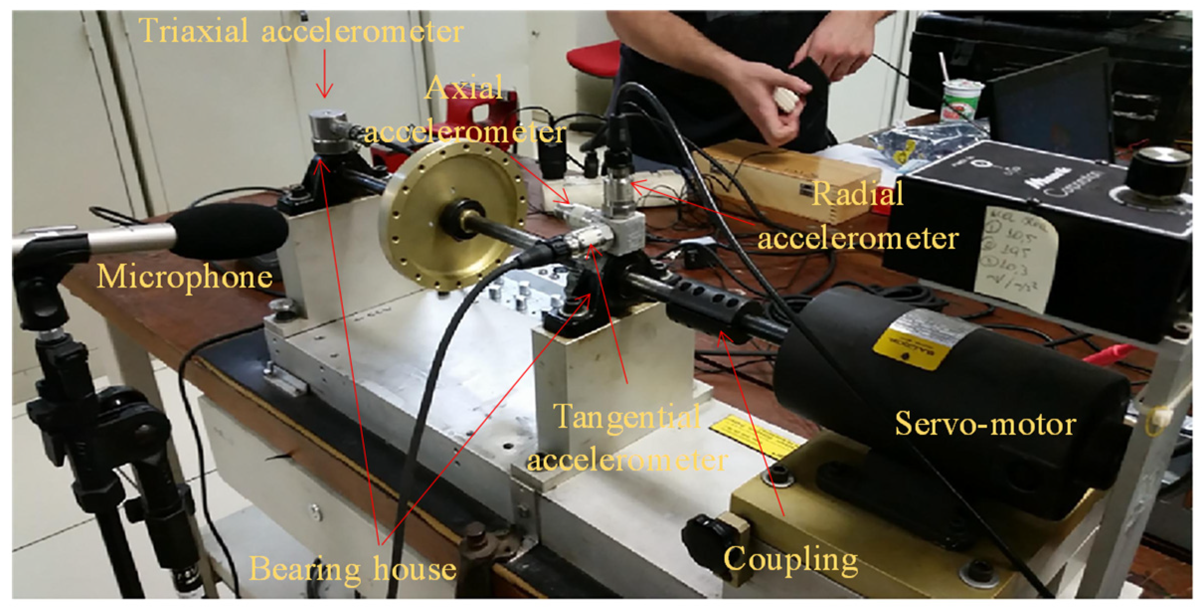
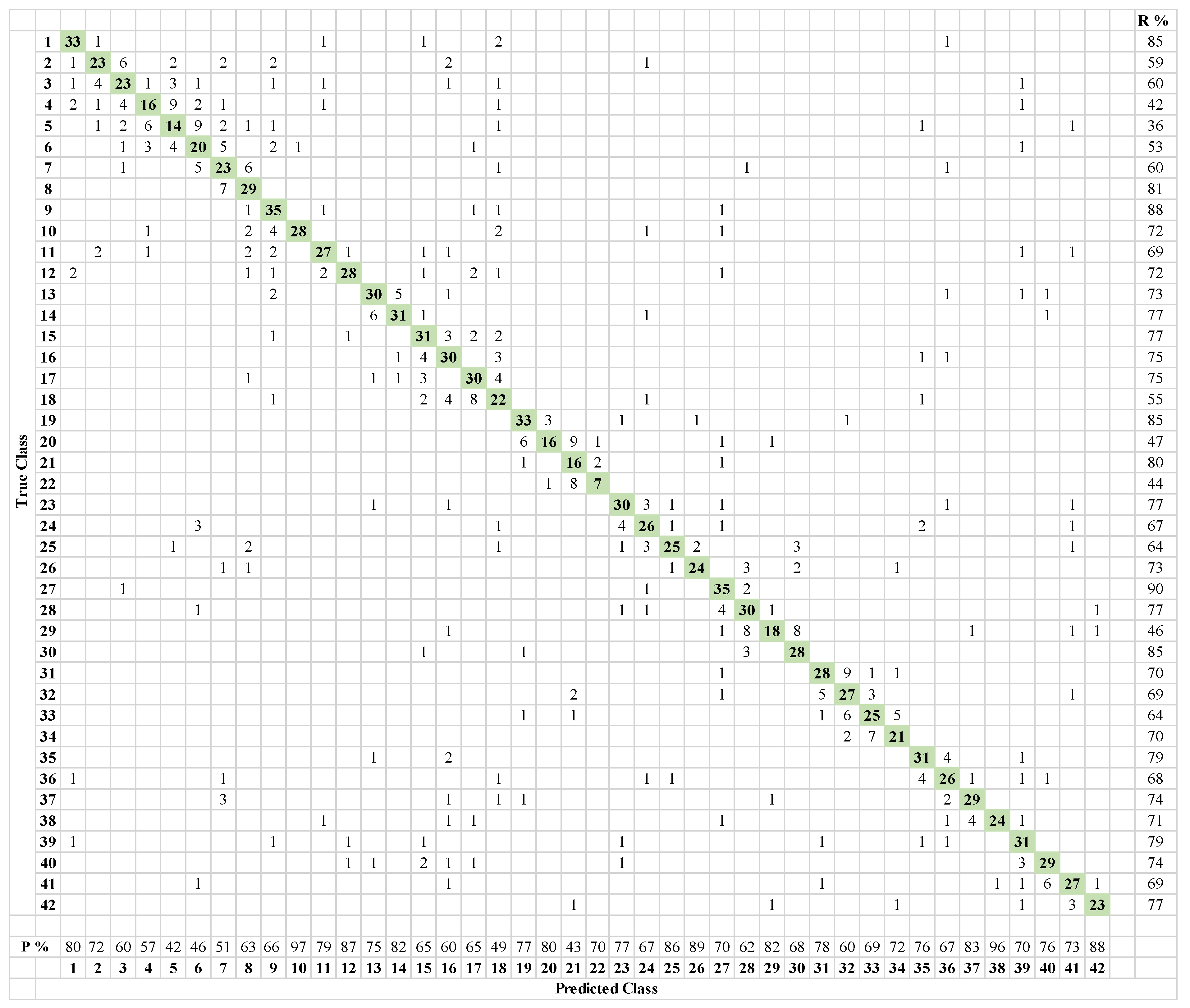
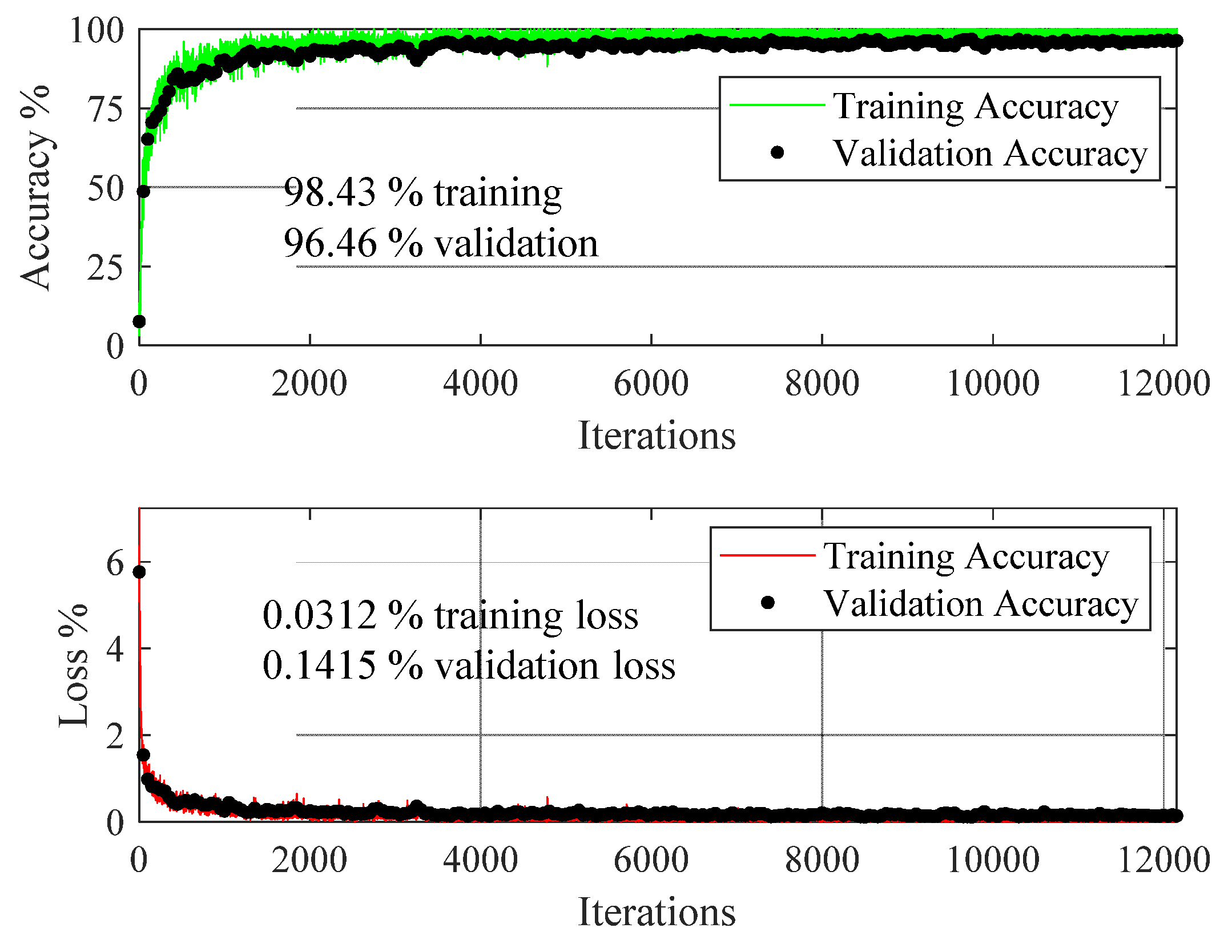
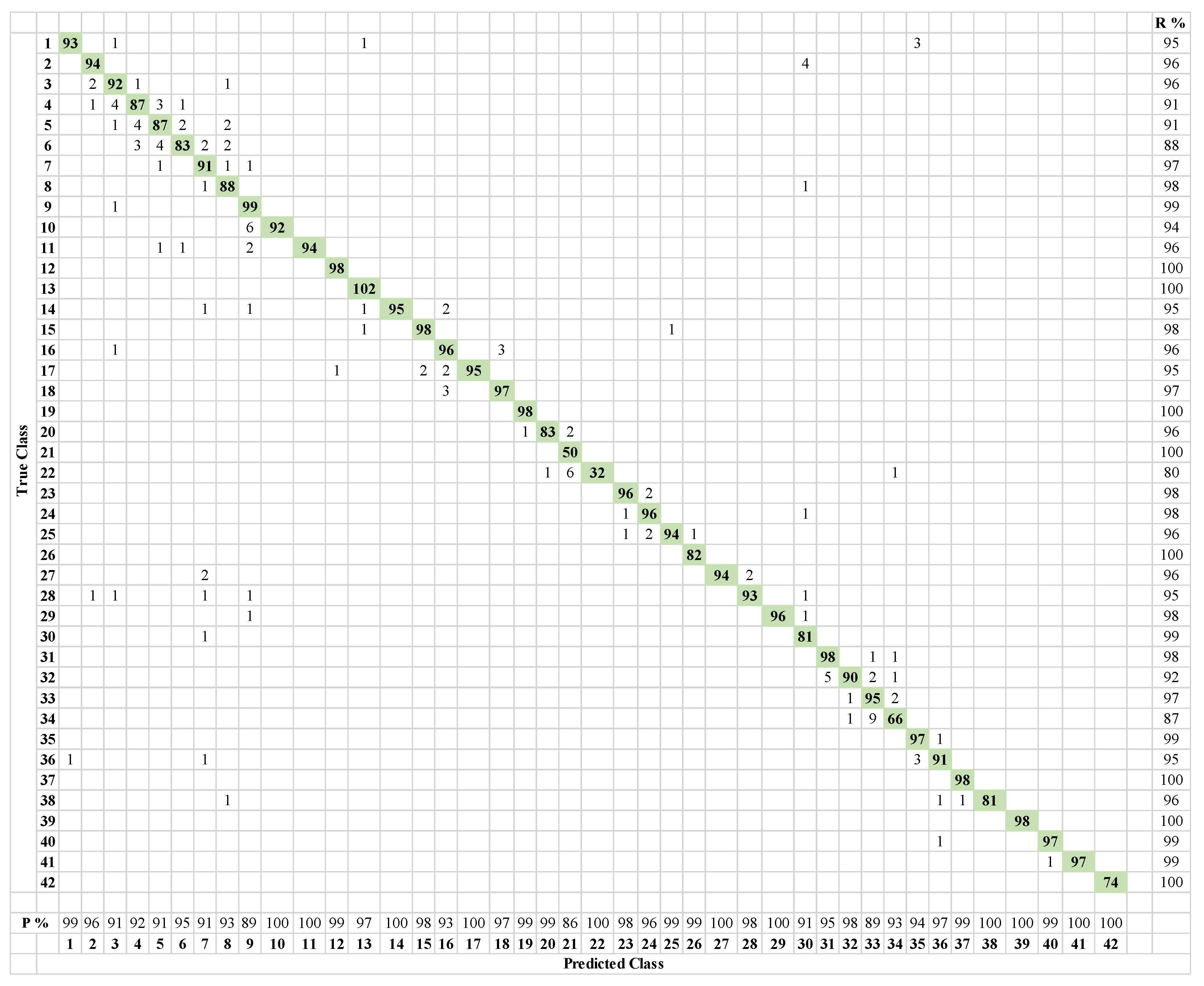
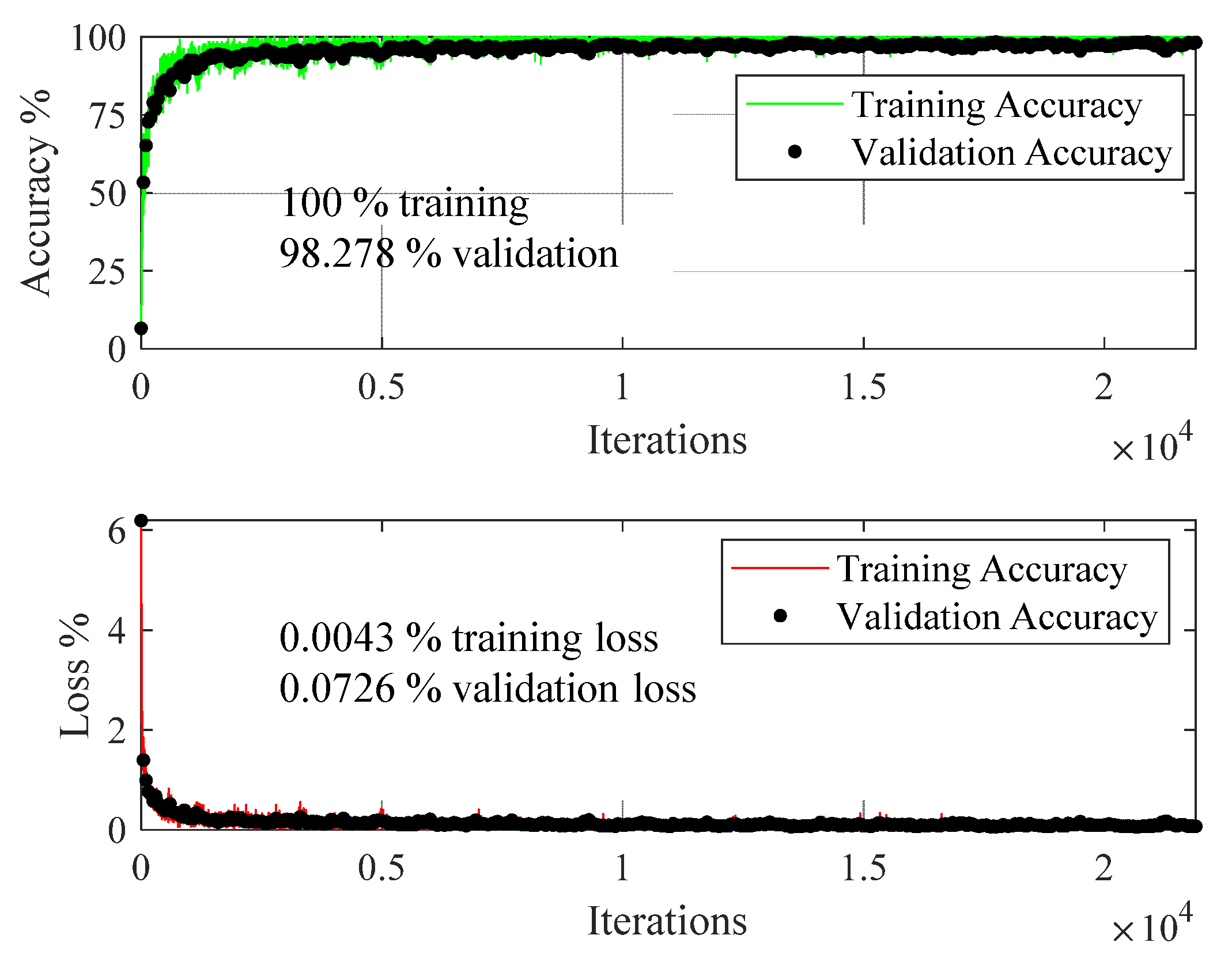
Table 1.
Summary of different health states.
| Health State | Severity Levels | Speed of Operation and Number of Measurements |
|---|---|---|
| Normal | No fault | 49 speeds (737 to 3886 rpm) Total 49 × 8 = 392 time series |
| Unbalance | 10 g, 15 g, 20 g, 25 g, 30 g, 35 g | 6 g >> 49 speeds, 10 g >> 48 speeds, 15 g >> 48 speeds 20 g >> 49 speeds, 25 g >> 47 speeds, 30 g >> 47 speeds 35 g >> 45 speeds (Total 333 × 8 = 2664 time series) |
| Horizontal Misalignment | 0.5 mm, 1.0 mm, 1.5 mm, 2.0 mm | 0.5 mm >> 50 speeds, 1.0 mm >> 49 speeds, 1.5 mm >> 49 speeds, 2 mm >> 49 speeds (Total 197 × 8 = 1576 time series) |
| Vertical Misalignment | 0.51 mm, 0.63 mm, 1.27 mm, 1.4 mm, 1.78 mm, 1.9 mm | 0.51 mm >> 51 speeds, 0.63 mm >> 50 speeds, 1.27 mm >> 50 speeds, 1.4 mm >> 50 speeds, 1.78 mm >> 50 speeds, 1.90 mm >> 50 speeds (301 × 8 = 2408 time series) |
| Bearing Faults | Underhang Position (between rotor and motor): Outer Race fault Rolling Element fault Inner Race fault | Outer race fault: {0 g >> 49 speeds, 6 g >> 48 speeds, 20 g >> 49 speeds, 35 g >> 42 speeds (188 × 8 = 1504 time series)} Rolling element fault: {0 g >> 49 speeds, 6 g >> 49 speeds, 20 g >> 49 speeds, 35 g >> 37 speeds (184 × 8 = 1472 time series)} Inner race fault: {0 g >> 50 speeds, 6 g >> 49 speeds, 20 g >> 49 speeds, 35 g >> 38 speeds (186 × 8 = 1488 time series)} |
| Overhang Position (rotor between bearing and motor): Outer Race fault Rolling Element fault Inner Race fault | Outer race fault: {0 g >> 49 speeds, 6 g >> 49 speeds, 20 g >> 49 speeds, 35 g >> 41 speeds (188 × 8 = 1504 time series)} Rolling element fault: {0 g >> 49 speeds, 6 g >> 49 speeds, 20 g >> 49 speeds, 35 g >> 41 speeds (188 × 8 = 1504 time series)} Inner race fault: {0 g >> 49 speeds, 6 g >> 43 speeds, 20 g >> 25 speeds, 35 g >> 20 speeds (137 × 8 = 1096 time series)} |
Table 2.
Summary of published literature using MafaulDa.
| # | Method | Type of Features | Results | Reference |
|---|---|---|---|---|
| 1 | Similarity-based modeling | Statistical time and frequency domain features | Classification of faults in general without considering severity of different defects | [48] |
| 2 | Optimize number of features and multilayer perceptron | Statistical Features | General classification of normal, unbalance, and misalignment only, without considering severity of different defects | [49] |
| 3 | Multilayer perceptron and division of normal state data | Fourier domain features | General classification of normal, unbalance, and misalignment only, without considering severity of different defects | [2] |
| 4 | Similarity based model and kernel discriminant analysis | Feature vector from discrete-time Fourier transform, kurtosis, and entropy of signal | Categorize the unbalance health state only into high, medium, and low | [50] |
| 5 | Synthetic minority over-sampling technique for imbalance class data | Statistical features and rotational frequency | Classification of faults in general without considering severity of different defects | [51] |
| 6 | Deep learning and t-SNE | Autonomous features from wavelet scalograms | Bearing faults classification only with the effect of unbalance mass on each defect | [52] |
| 7 | Ensemble convolutional neural network (EnCNN) | Autonomous feature extraction from sensor signals | Fault classification using normal, horizontal misalignment and vertical misalignment data with severities. | [47] |
Table 3.
Architectural details of the customized deep learning model.
| Layer Name | Description |
|---|---|
| image input layer | 100 × 100 × 3 Scalograms |
| Convolution 1, Pooling 1 | Convolution layer (Filter 3 × 3, 16 Filters) |
| Batch Normalization | |
| ReLU layer | |
| Max-pooling Layer (Filter 2 × 2, strides 2) | |
| Convolution 2, Pooling 2, drop-out 1 | Convolution layer (Filter 3 × 3, 32 Filters) |
| Batch Normalization | |
| ReLU layer | |
| Max-pooling Layer (Filter 2 × 2, strides 2) | |
| dropout layer (0.2 drop out probability) | |
| Convolution 3, drop-out 2 | Convolution layer (Filter 3 × 3, 48 Filters) |
| Batch Normalization | |
| ReLU layer | |
| dropout layer (0.2 drop out probability) | |
| Convolution 4, Pooling 4, drop-out 3 | Convolution layer (Filter 3 × 3, 64 Filters) |
| Batch Normalization | |
| ReLU layer | |
| Max-pooling Layer (Filter 2 × 2, strides 2) | |
| dropout layer (0.2 drop out probability) | |
| Convolution 5, drop-out 5 | Convolution layer (Filter 3 × 3, 64 Filters) |
| Batch Normalization | |
| ReLU layer | |
| dropout layer (0.2 drop out probability) | |
| Convolution 6 | Convolution layer (Filter 3 × 3, 64 Filters) |
| Batch Normalization | |
| ReLU layer | |
| Global pooling | Max-pooling Layer ([1 13]) |
| Fully connected layer | 42 classes |
| classification layer | with SoftMax function for classification |
Table 4.
Improvement in the classification performance due to data augmentation in comparison with the original data without augmentation.
Table 4.
Improvement in the classification performance due to data augmentation in comparison with the original data without augmentation.
| Network | Training Accuracy% | Validation Accuracy% | Training Loss% | Validation Loss% |
|---|---|---|---|---|
| ResNet18 (8 virtual sensors) | Increased by 5.87 | Increased by 43.97 | Decreased by 86.96 | Decreased by 91.5 |
| Customized CNN (8 virtual sensors) | Increased by 7.56 | Increased by 46.68 | Decreased by 98.2 | Decreased by 95.64 |
| ResNet18 (16 virtual sensors) | Increased by 15.3 | Increased by 49.2 | Decreased by 94.9 | Decreased by 93.5 |
| Customized CNN (16 virtual sensors) | Increased by 14.4 | Increased by 41.5 | Decreased by 86.5 | Decreased by 92.0 |
Publisher’s Note: MDPI stays neutral with regard to jurisdictional claims in published maps and institutional affiliations. |
© 2021 by the authors. Licensee MDPI, Basel, Switzerland. This article is an open access article distributed under the terms and conditions of the Creative Commons Attribution (CC BY) license (https://creativecommons.org/licenses/by/4.0/).
Share and Cite
MDPI and ACS Style
Khan, A.; Hwang, H.; Kim, H.S. Synthetic Data Augmentation and Deep Learning for the Fault Diagnosis of Rotating Machines. Mathematics 2021, 9, 2336. https://0-doi-org.brum.beds.ac.uk/10.3390/math9182336
AMA Style
Khan A, Hwang H, Kim HS. Synthetic Data Augmentation and Deep Learning for the Fault Diagnosis of Rotating Machines. Mathematics. 2021; 9(18):2336. https://0-doi-org.brum.beds.ac.uk/10.3390/math9182336
Chicago/Turabian StyleKhan, Asif, Hyunho Hwang, and Heung Soo Kim. 2021. "Synthetic Data Augmentation and Deep Learning for the Fault Diagnosis of Rotating Machines" Mathematics 9, no. 18: 2336. https://0-doi-org.brum.beds.ac.uk/10.3390/math9182336
Note that from the first issue of 2016, this journal uses article numbers instead of page numbers. See further details here.