Figure 1.
Geometry of the flow problem.
Figure 1.
Geometry of the flow problem.
Figure 2.
Total residual error with , , , , , , , , and .
Figure 2.
Total residual error with , , , , , , , , and .
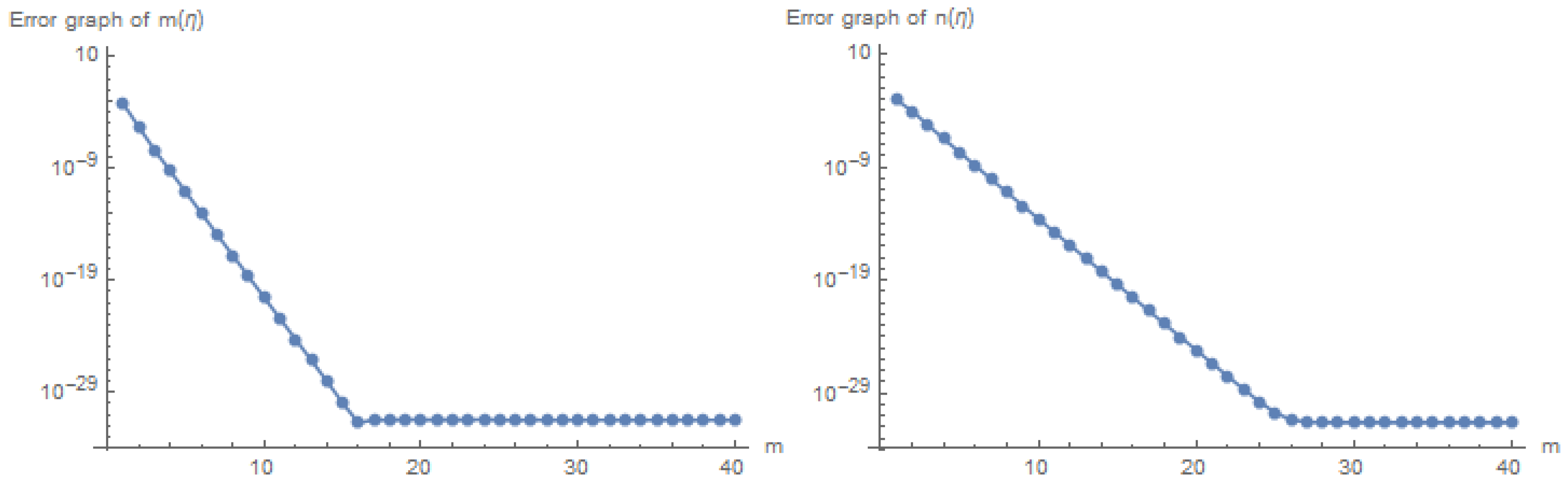
Figure 3.
Error profile for and with , , , , , , , , and .
Figure 3.
Error profile for and with , , , , , , , , and .
Figure 4.
Error profile for and with , , , , , , , , and .
Figure 4.
Error profile for and with , , , , , , , , and .
Figure 5.
Error profile for and with , , , , , , , , and .
Figure 5.
Error profile for and with , , , , , , , , and .
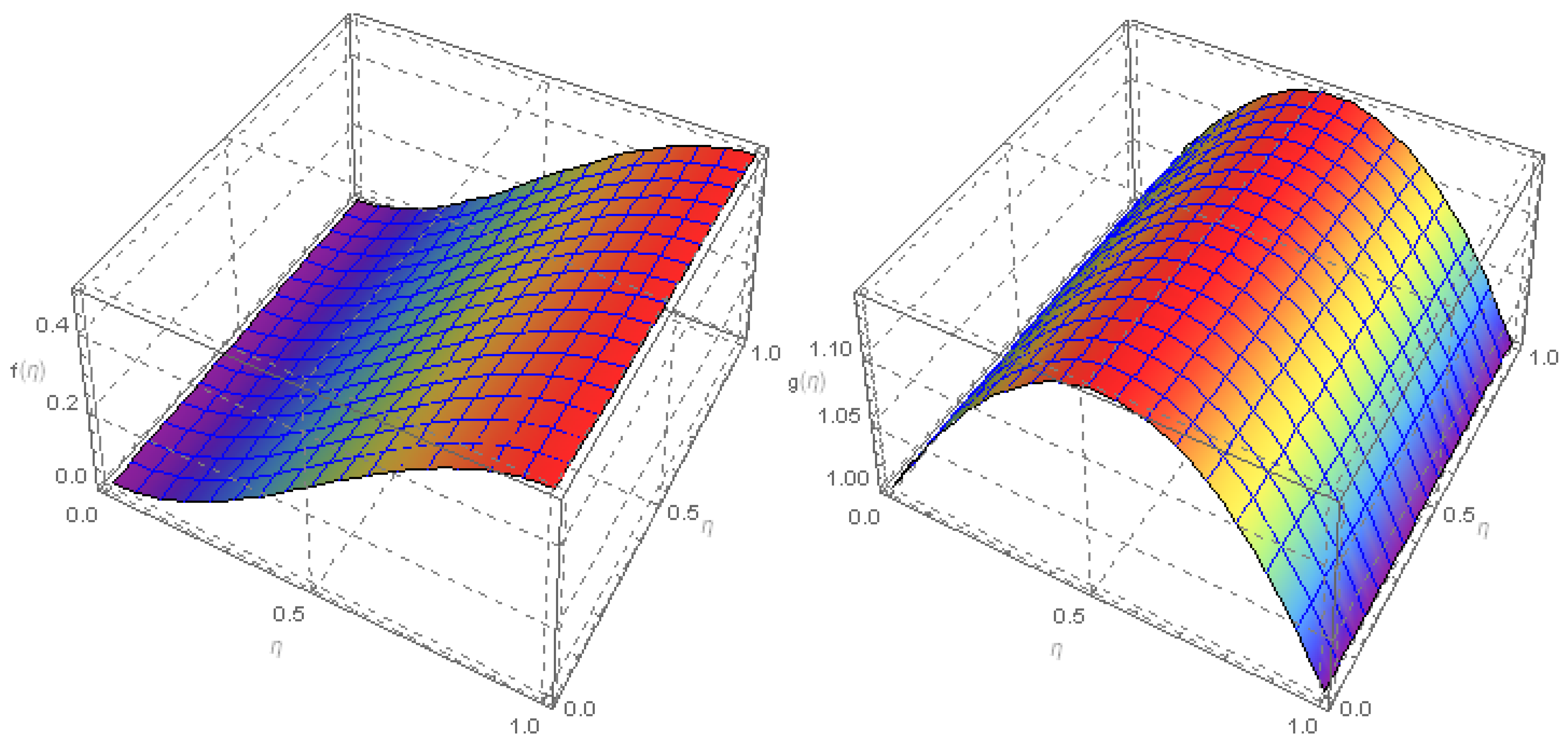
Figure 6.
3D graph for and with , , , , , , , , and .
Figure 6.
3D graph for and with , , , , , , , , and .
Figure 7.
3D graph for and with , , , , , , , , and .
Figure 7.
3D graph for and with , , , , , , , , and .
Figure 8.
3D graph for and with , , , , , , , , and .
Figure 8.
3D graph for and with , , , , , , , , and .
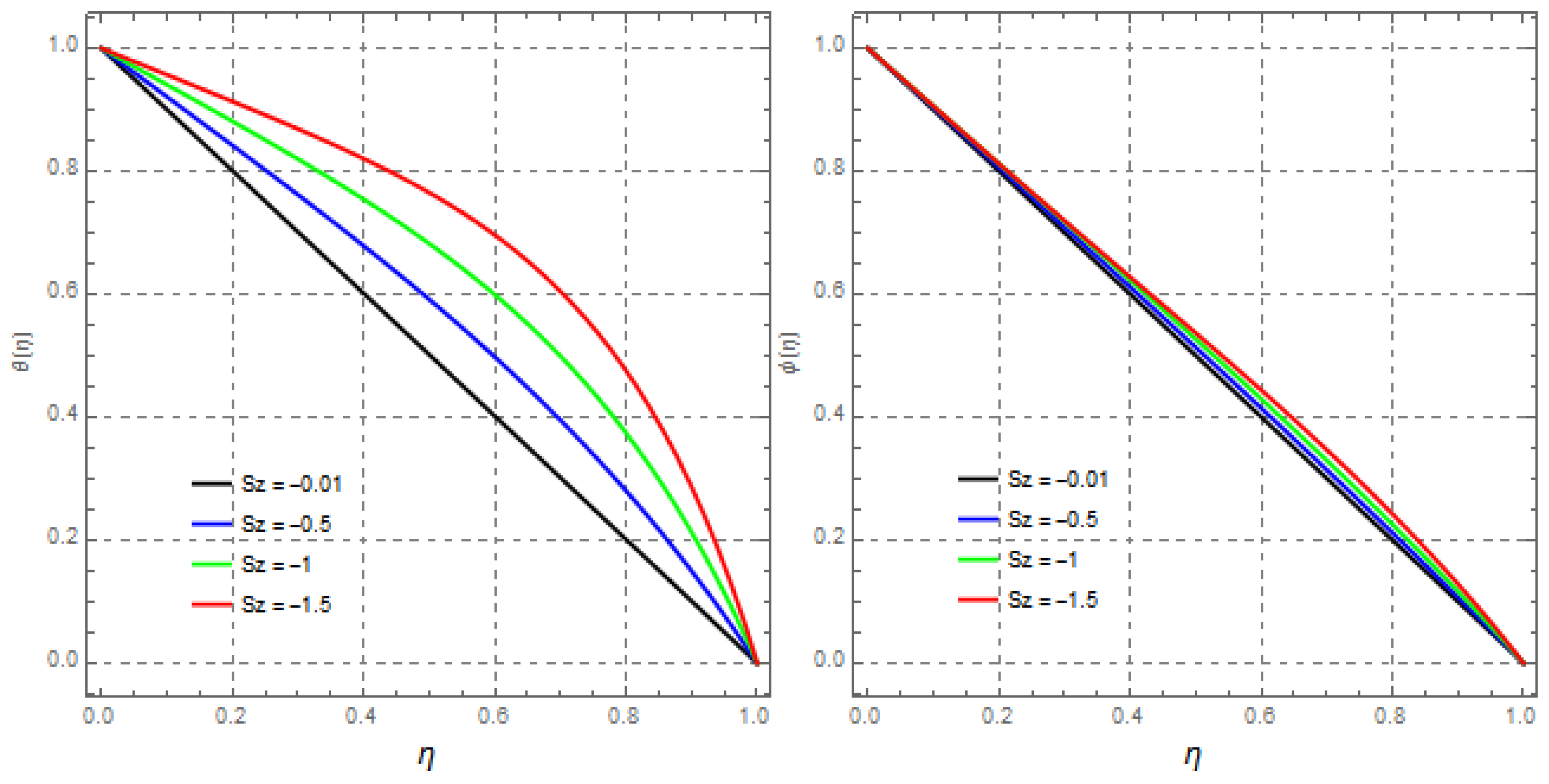
Figure 9.
Impact of squeeze Reynold number on and , keeping , , , ,, , , and .
Figure 9.
Impact of squeeze Reynold number on and , keeping , , , ,, , , and .
Figure 10.
Observing the effect of squeeze Reynold number on and with , , , , , , , and .
Figure 10.
Observing the effect of squeeze Reynold number on and with , , , , , , , and .
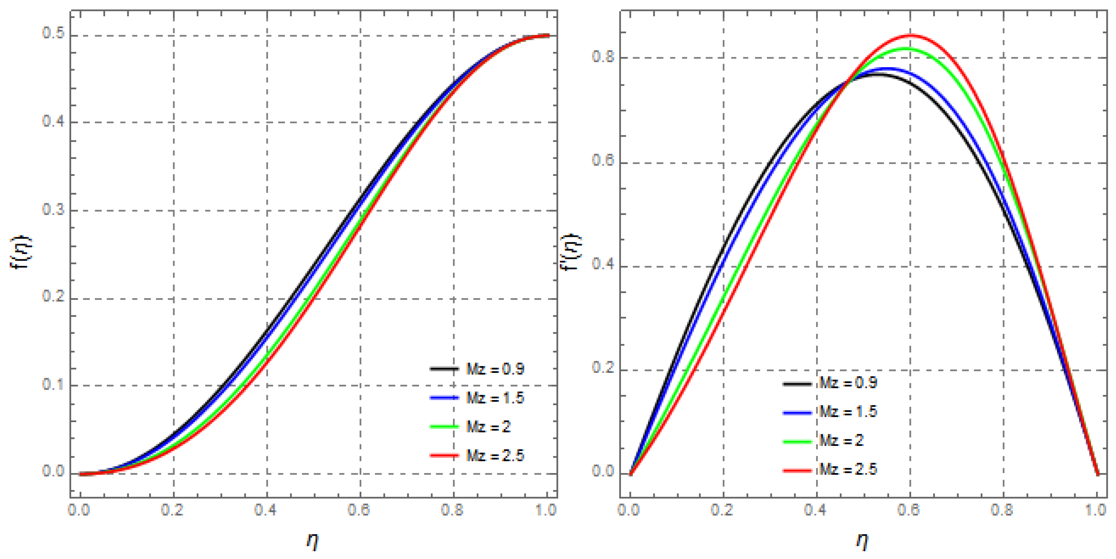
Figure 11.
Impact of squeeze Reynold number on , keeping , , , , , , , and .
Figure 11.
Impact of squeeze Reynold number on , keeping , , , , , , , and .
Figure 12.
Observing the effect of squeeze Reynold number on and with , , , , , , , and .
Figure 12.
Observing the effect of squeeze Reynold number on and with , , , , , , , and .
Figure 13.
Observing the effect of magnetic strength parameter on and with , , , , , , , and .
Figure 13.
Observing the effect of magnetic strength parameter on and with , , , , , , , and .
Figure 14.
Observing the effect of magnetic strength parameter on and with , , , , , , , and .
Figure 14.
Observing the effect of magnetic strength parameter on and with , , , , , , , and .
Figure 15.
Observing the effect of magnetic strength parameter on with , , , , , , , and .
Figure 15.
Observing the effect of magnetic strength parameter on with , , , , , , , and .
Figure 16.
Observing the effect of magnetic strength parameter on and with , , , , , , , and .
Figure 16.
Observing the effect of magnetic strength parameter on and with , , , , , , , and .
Figure 17.
Observing the effect of magnetic strength parameter on with , , , , , , , and .
Figure 17.
Observing the effect of magnetic strength parameter on with , , , , , , , and .
Figure 18.
Observing the effect of magnetic strength parameter on with , , , , , , , and .
Figure 18.
Observing the effect of magnetic strength parameter on with , , , , , , , and .
Figure 19.
Observing the effect of magnetic Reynold number on and with , , , , , , , and .
Figure 19.
Observing the effect of magnetic Reynold number on and with , , , , , , , and .
Figure 20.
Observing the effect of magnetic Reynold number on and with , , , , , , , and .
Figure 20.
Observing the effect of magnetic Reynold number on and with , , , , , , , and .
Figure 21.
Observing the effect of magnetic Reynold number on with , , , , , , , and .
Figure 21.
Observing the effect of magnetic Reynold number on with , , , , , , , and .
Figure 22.
Observing the effect of magnetic Reynold number on and with , , , , , , , and .
Figure 22.
Observing the effect of magnetic Reynold number on and with , , , , , , , and .
Figure 23.
Observing the effect of squeeze Dufour number on and with , , , , , , , and .
Figure 23.
Observing the effect of squeeze Dufour number on and with , , , , , , , and .
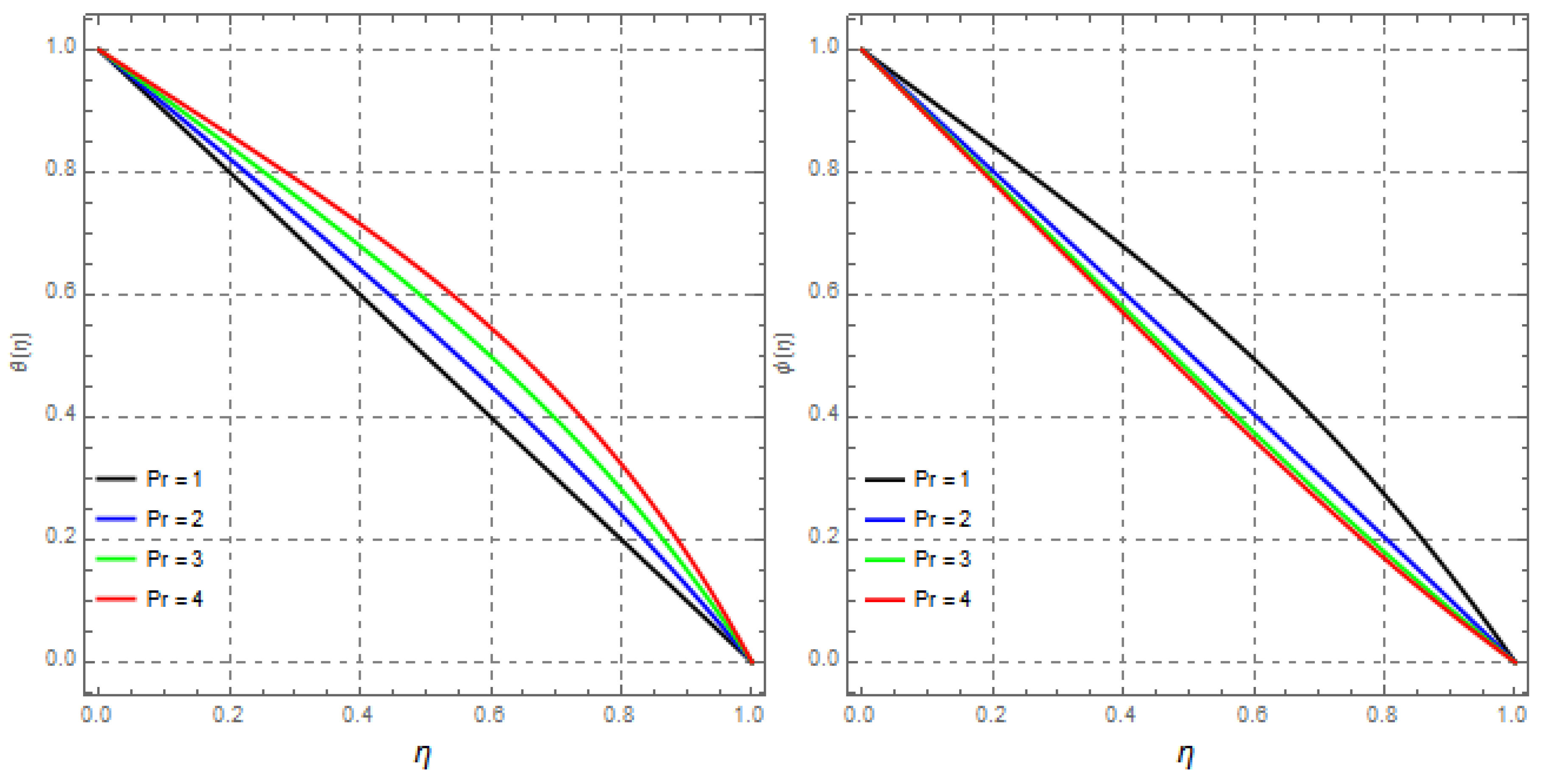
Figure 24.
Observing the effect of Prandtl number on and with , , , , , , , and .
Figure 24.
Observing the effect of Prandtl number on and with , , , , , , , and .
Figure 25.
Observing the effect of Soret number on and with , , , , , , , and .
Figure 25.
Observing the effect of Soret number on and with , , , , , , , and .
Figure 26.
Observing the effect of radiation parameter on and with , , , , , , , and .
Figure 26.
Observing the effect of radiation parameter on and with , , , , , , , and .
Figure 27.
Observing the effect of Schmidt number on and with , , , , , , , , and .
Figure 27.
Observing the effect of Schmidt number on and with , , , , , , , , and .
Table 1.
Estimating the total residual error for different orders of approximation.
Table 1.
Estimating the total residual error for different orders of approximation.
| m | | | | | | |
|---|
| 1 | 0.03811 | 0.00475 | 0.00066 | 0.00088 | 8.4 | 1.0 |
| 5 | 1.5 | 1.0 | 7.6 | 2.1 | 1.5 | 3.3 |
| 10 | 1.0 | 9.5 | 2.8 | 2.7 | 4.6 | 1.2 |
| 15 | 5.9 | 1.0 | 1.2 | 4.1 | 1.0 | 3.0 |
| 20 | 2.8 | 1.3 | 2.8 | 6.5 | 2.4 | 1.0 |
| 25 | 2.8 | 1.8 | 4.5 | 1.6 | 6.0 | 6.8 |
| 30 | 2.9 | 1.2 | 3.0 | 1.5 | 6.2 | 6.8 |
| 35 | 2.9 | 1.2 | 3.0 | 1.5 | 6.2 | 6.8 |
| 40 | 2.9 | 1.2 | 3.0 | 1.5 | 6.2 | 6.8 |
Table 2.
Optimal values of convergence control parameters in comparison of different orders of approximation.
Table 2.
Optimal values of convergence control parameters in comparison of different orders of approximation.
| Order | | | | | | | |
|---|
| 2 | −1.0151 | −1.0459 | −0.8810 | −0.7341 | −0.1047 | −0.1040 | 0.00203 |
| 3 | −0.9471 | −1.1027 | −0.9423 | −0.8706 | −0.1110 | −1.0261 | 4.90 |
| 4 | −0.9678 | −1.0804 | −0.9360 | −0.8889 | −0.1053 | −0.9786 | 4.94 |
| 5 | −0.9290 | −1.0601 | −0.9433 | −0.9223 | −0.1140 | −1.0579 | 2.20 |
| 6 | −0.9583 | −1.0441 | −0.9435 | −0.9342 | −0.1369 | −1.0050 | 2.87 |
| 7 | −1.1097 | −1.0693 | −0.8652 | −0.9240 | −0.1172 | −1.0967 | 3.26 |
Table 3.
Estimated values for velocity, magnetic field components, temperature and concentration in correspondance with different values of .
Table 3.
Estimated values for velocity, magnetic field components, temperature and concentration in correspondance with different values of .
| | | | | | |
|---|
| 0 | 0 | 1 | 0 | 0 | 1 | 1 |
| 0.1 | 0.013945 | 1.038790 | 0.083334 | 0.090262 | 0.899994 | 0.899811 |
| 0.2 | 0.051898 | 1.070930 | 0.167626 | 0.179204 | 0.799991 | 0.799707 |
| 0.3 | 0.107937 | 1.095050 | 0.253977 | 0.268342 | 0.699991 | 0.699719 |
| 0.4 | 0.176060 | 1.110120 | 0.343567 | 0.359189 | 0.599995 | 0.599833 |
| 0.5 | 0.250219 | 1.115470 | 0.437564 | 0.453152 | 0.500000 | 0.500005 |
| 0.6 | 0.324349 | 1.110810 | 0.537016 | 0.551440 | 0.400006 | 0.400177 |
| 0.7 | 0.392389 | 1.096270 | 0.642747 | 0.654974 | 0.300009 | 0.300290 |
| 0.8 | 0.448305 | 1.072300 | 0.755239 | 0.764292 | 0.200010 | 0.200299 |
| 0.9 | 0.486125 | 1.039810 | 0.874512 | 0.879464 | 0.100006 | 0.100192 |
| 1 | 0.5 | 1 | 1 | 1 | 0 | 0 |
Table 4.
The convergence of HAM solution for skin friction, magnetic flux, heat flux and mass flux.
Table 4.
The convergence of HAM solution for skin friction, magnetic flux, heat flux and mass flux.
| m | | | | | | |
|---|
| 1 | 2.9631400 | −0.3922459 | 0.8311292 | −0.9204676 | 1.0000650 | 1.0020067 |
| 5 | 2.9804441 | −0.4157942 | −0.8318657 | −0.9141364 | 1.0000668 | 1.0020675 |
| 10 | 2.9804441 | −0.4157877 | −0.8318658 | −0.9141418 | 1.0000668 | 1.002067 |
| 15 | 2.9804441 | −0.4157877 | −0.8318658 | −0.9141418 | 1.0000668 | 1.002067 |
| 20 | 2.9804441 | −0.4157877 | −0.8318658 | −0.9141418 | 1.0000668 | 1.002067 |
| 25 | 2.9804441 | −0.4157877 | −0.8318658 | −0.9141418 | 1.0000668 | 1.002067 |
| 30 | 2.9804441 | −0.4157877 | −0.8318658 | −0.9141418 | 1.0000668 | 1.002067 |
| 35 | 2.9804441 | −0.4157877 | −0.8318658 | −0.9141418 | 1.0000668 | 1.002067 |
| 40 | 2.9804441 | −0.4157877 | −0.8318658 | −0.9141418 | 1.0000668 | 1.002067 |
Table 5.
Effect of on skin friction, magnetic flux, heat flux and mass flux.
Table 5.
Effect of on skin friction, magnetic flux, heat flux and mass flux.
| | | | | | |
|---|
| −0.01 | 2.999403 | −0.017073 | −0.831885 | −0.569941 | 0.999976 | 0.999247 |
| −0.25 | 2.985167 | −0.467599 | −0.831912 | −0.553833 | 0.999397 | 0.981150 |
| −0.75 | 2.956173 | −1.768705 | −0.831980 | −0.505905 | 0.998187 | 0.943287 |
| −1.25 | 2.928189 | −4.069057 | −0.832065 | −0.418285 | 0.996968 | 0.905179 |
Table 6.
Effect of on skin friction, magnetic flux, heat flux and mass flux.
Table 6.
Effect of on skin friction, magnetic flux, heat flux and mass flux.
| | | | | | |
|---|
| 1 | 2.985167 | −0.457030 | −0.831912 | −0.121005 | 0.999397 | 0.981150 |
| 3 | 2.985167 | −0.467600 | −0.831912 | −0.553832 | 0.999397 | 0.981150 |
| 5 | 2.985167 | −0.478166 | −0.831912 | −0.640398 | 0.999397 | 0.981150 |
| 7 | 2.985167 | −0.488735 | −0.831912 | −0.677498 | 0.999397 | 0.981150 |
Table 7.
Effect of on skin friction, magnetic flux, heat flux and mass flux.
Table 7.
Effect of on skin friction, magnetic flux, heat flux and mass flux.
| | | | | | |
|---|
| 1 | 2.980444 | −0.415788 | −0.831866 | −0.914141 | 0.999398 | 0.981167 |
| 1.5 | 2.985167 | −0.435894 | −0.831912 | −0.986660 | 0.999397 | 0.981150 |
| 2 | 2.991858 | −0.466561 | −0.831978 | −1.060309 | 0.999397 | 0.981125 |
| 2.5 | 3.000600 | −0.508235 | −0.832064 | −1.135544 | 0.999396 | 0.981093 |
Table 8.
Effect of on skin friction, magnetic flux, heat flux and mass flux.
Table 8.
Effect of on skin friction, magnetic flux, heat flux and mass flux.
| | | | | | |
|---|
| 0.1 | 2.976998 | −0.408251 | −0.962689 | −0.921462 | 0.998762 | 0.981100 |
| 0.5 | 2.977633 | −0.414660 | −0.831838 | −0.663347 | 0.998762 | 0.981098 |
| 1 | 2.977560 | −0.419649 | −0.701154 | −0.433268 | 0.998762 | 0.981097 |
| 1.5 | 2.976902 | −0.422670 | −0.597416 | −0.271630 | 0.998762 | 0.981099 |
Table 9.
Effect of on skin friction, magnetic flux, heat flux and mass flux.
Table 9.
Effect of on skin friction, magnetic flux, heat flux and mass flux.
| | | | | | |
|---|
| 0.1 | 2.985167 | −0.467599 | −0.831912 | −0.553833 | 0.999236 | 0.981129 |
| 0.75 | 2.985167 | −0.467599 | −0.831912 | −0.553833 | 0.999498 | 0.981162 |
| 1.25 | 2.985167 | −0.467599 | −0.831912 | −0.553833 | 0.999699 | 0.981188 |
| 1.75 | 2.985167 | −0.467599 | −0.831912 | −0.553833 | 0.999900 | 0.981213 |
Table 10.
Effect of on skin friction, magnetic flux, heat flux and mass flux.
Table 10.
Effect of on skin friction, magnetic flux, heat flux and mass flux.
| | | | | | |
|---|
| 0.1 | 2.977633 | −0.414660 | −0.831838 | −0.663347 | 0.998762 | 0.981098 |
| 0.5 | 2.977633 | −0.414660 | −0.831838 | −0.663347 | 0.999158 | 0.981147 |
| 1 | 2.977633 | −0.414660 | −0.831838 | −0.663347 | 0.999398 | 0.981177 |
| 1.5 | 2.977633 | −0.414660 | −0.831838 | −0.663347 | 0.999532 | 0.981194 |
Table 11.
Effect of on skin friction, magnetic flux, heat flux and mass flux.
Table 11.
Effect of on skin friction, magnetic flux, heat flux and mass flux.
| | | | | | |
|---|
| 0.05 | 2.977633 | −0.414660 | −0.831838 | −0.663347 | 0.999532 | 0.981194 |
| 0.1 | 2.977633 | −0.414660 | −0.831838 | −0.663347 | 0.999064 | 0.981135 |
| 0.25 | 2.977633 | −0.414660 | −0.831838 | −0.663347 | 0.997668 | 0.980960 |
| 0.5 | 2.977633 | −0.414660 | −0.831838 | −0.663347 | 0.995361 | 0.980671 |
Table 12.
Effect of on skin friction, magnetic flux, heat flux and mass flux.
Table 12.
Effect of on skin friction, magnetic flux, heat flux and mass flux.
| | | | | | |
|---|
| 0.1 | 3.000040 | −0.222019 | −0.831954 | −0.622051 | 0.999758 | 0.992499 |
| 0.5 | 3.000040 | −0.222019 | −0.831954 | −0.622051 | 0.999758 | 0.992548 |
| 1 | 3.000040 | −0.222019 | −0.831954 | −0.622051 | 0.999758 | 0.992609 |
| 1.5 | 3.000040 | −0.222019 | −0.831954 | −0.622051 | 0.999757 | 0.992670 |
Table 13.
Effect of on skin friction, magnetic flux, heat flux and mass flux.
Table 13.
Effect of on skin friction, magnetic flux, heat flux and mass flux.
| | | | | | |
|---|
| 0.5 | 2.985167 | −0.478167 | −0.831912 | −0.640398 | 0.999397 | 0.981150 |
| 1 | 2.985167 | −0.478167 | −0.831912 | −0.640398 | 0.999598 | 0.962350 |
| 1.5 | 2.985167 | −0.478167 | −0.831912 | −0.640398 | 0.999799 | 0.943600 |
| 2 | 2.985167 | −0.478167 | −0.831912 | −0.640398 | 1.000000 | 0.924901 |


