New Importance Measures Based on Failure Probability in Global Sensitivity Analysis of Reliability

Abstract

This article presents new sensitivity measures in reliability-oriented global sensitivity analysis. The obtained results show that the contrast and the newly proposed sensitivity measures (entropy and two others) effectively describe the influence of input random variables on the probability of failure P_f. The contrast sensitivity measure builds on Sobol, using the variance of the binary outcome as either a success (0) or a failure (1). In Bernoulli distribution, variance P_f(1 − P_f) and discrete entropy—P_fln(P_f) − (1 − P_f)ln(1 − P_f) are similar to dome functions. By replacing the variance with discrete entropy, a new alternative sensitivity measure is obtained, and then two additional new alternative measures are derived. It is shown that the desired property of all the measures is a dome shape; the rise is not important. Although the decomposition of sensitivity indices with alternative measures is not proven, the case studies suggest a rationale structure of all the indices in the sensitivity analysis of small P_f. The sensitivity ranking of input variables based on the total indices is approximately the same, but the proportions of the first-order and the higher-order indices are very different. Discrete entropy gives significantly higher proportions of first-order sensitivity indices than the other sensitivity measures, presenting entropy as an interesting new sensitivity measure of engineering reliability.

1. Introduction

The reliability-oriented sensitivity analysis (ROSA) differs from the classical sensitivity analysis in the subject of interest. Classical sensitivity analysis focuses on the model output, whereas the ROSA generally deals with reliability measures, usually the failure probability P_f [1].

In civil engineering, the numerical analysis of small P_f using conventional stochastic models is very time-consuming [2]. Although the probability analysis of structural reliability is constantly evolving [3,4,5], the development of the ROSA is lagging.

In a multidisciplinary context, the mainstream global sensitivity analysis (SA) focuses on model outputs [6]. In civil engineering, the global SA is used to study model outputs of surrogate models without a direct relationship to P_f, with the results reflecting model simplifications of approximation methods [7,8,9,10].

The global ROSA directly aimed at P_f was developed relatively recently [11,12,13]. Articles [11,12] present sensitivity indices oriented to the probability of failure, which is based on the decomposition of the variance of a binary function (failure, success), building on Sobol [14,15] where the sum of all the indices is equal to one and each index is non-negative. The same indices can be obtained using the contrast function [13] where P_f is a minimizer. The rationality of sensitivity indices [11,12,13] has been shown in many applications [16,17,18,19,20,21,22,23,24,25].

Other ROSA methods have drawbacks that reduce their generality. The derivative P_f measures only local change at the derivative point [26]. Methods [27,28] oriented to the reliability index β cannot analyze the interaction effects of input variables. According to the Bayes formula, the SA in [29] analyzes P_f using first- and second-order sensitivity indices, but without the introduction of the higher orders. The following method avoids the nested sampling procedure, but only the first-order sensitivity indices have been introduced so far [30,31]. The method in [32] represents the SA of P_f using sensitivity indices of all the orders which do not have the sum of all the indices equal to one. The SA in [33] studies P_f, but in order to identify new training points for the surrogate models. None of the indices in [26,27,28,29,30,31,32,33] is based on decomposition as in the variance-based global SA. As the comparative studies of [34] have shown, the values of sensitivity indices can vary greatly depending on the type of ROSA used.

In the reliability analysis of a structure, the system is characterized by two possible results: unreliability and reliability [35,36]. Although reliability can be assessed without P_f using design quantiles, the SA of design quantiles cannot calculate the interaction effects between load and resistance [37,38,39,40]. The correlation methods [41,42], Sobol SA [14,15]; density-based SA [43,44]; entropy-based SA [45,46]; quantile-based SA [47,48] and [37,38,39,40]; SA in Multiple Criteria Decision Making (MCDM) [49,50]; and other SA types [51,52] are effective in their applications, but may not work properly in reliability tasks.

Numerous probabilistic sensitivity measures have been presented in a multidisciplinary context [53,54,55]. However, the mere fact that sensitivity measures are moment-independent does not mean that they are reliability-oriented. The effect of an input variable on the distribution of the output is not equal to the effect on the P_f [56].

Reliability and sensitivity analyses should work in tandem with a common focus on P_f. The goal of the ROSA should be P_f, including all interaction effects from input random variables. This article presents new global sensitivity measures oriented to P_f, building on Sobol [14,15] on the path from variance [11,12,13] to entropy and other measures. The research presents case studies with induction from results starting from the particular to the more general.

2. Sobol Sensitivity Analysis

The Sobol SA of model output [14,15] is very popular and has been applied in many engineering studies; see, e.g., [57,58,59,60,61,62,63]. The basic concept can be introduced as follows.

Let us consider a response function f with output Y with continuous input random variables (X₁, X₂,…, X_M).

$$Y\left(X\right)=f\left(X_1,X_2,..\hspace{0.33em},X_i,..\hspace{0.33em},X_M\right).$$

(1)

The Function (1) is assumed to be integrable in Ω^M:

$${\Omega }^M=\left(X\left|0\le x_i\le 1;\hspace{0.33em}i=1;\hspace{0.33em}\dots ,\hspace{0.33em}M\right.\right).$$

(2)

Sobol’s concept decomposes the response function (1) into a form with increasing dimension:

$$f=f_0+{\displaystyle \sum _i{f}_i}\left(X_i\right)+{\displaystyle \sum _i{\displaystyle \sum _{j>i}{f}_{ij}\left(X_i,X_j\right)}}+\dots +f_{12\dots M}\left(X_1,X_2,\dots ,X_M\right),$$

(3)

where the number of members is 2^M. Each input random variable X_i has the probability density function (pdf) φ_i(x_i) ≥ 0 defined on the interval [0, 1], otherwise φ_i(x_i) = 0. Assuming the statistical independence of the input variables, the multivariate distributions equal the product of the marginal distributions. Fubini’s theorem on double integrals implies that if each member of the decomposition (apart from the constant f₀) has a mean value of zero

$$E\left(f\left(x_i\right)\right)={\displaystyle \underset{0}{\overset{1}{\int }}{\phi }_i\left(x_i\right)\cdot f\left(x_i\right)d{x}_i}=0,$$

(4)

then all the members of the decomposition are orthogonal in pairs:

$$E\left(f\left(x_i\right)\cdot f\left(x_j\right)\right)=\underset{0}{\overset{1}{\int }}\underset{0}{\overset{1}{\int }}{\phi }_i\left(x_i\right)\cdot f\left(x_i\right)\cdot {\phi }_j\left(x_j\right)\cdot f\left(x_j\right)d{x}_{i}d{x}_j=0, i\ne j.$$

(5)

The members of the decomposition (3) can therefore be expressed using the conditional realization of the model output.

$$f_0=E\left(Y\right),$$

(6)

$$f_i\left(X_i\right)=E\left(Y\left|X_i\right.\right) -f_0,$$

(7)

$$f_{ij}\left(X_i,X_j\right)=E\left(Y\left|X_i\right.,\hspace{0.33em}{X}_j\right) -f_i-f_j-f_0.$$

(8)

In Equation (3), due to orthogonality, the members of the decomposition are statistically independent random variables, where the sum of the variances of the individual members is equal to the variance of the output; see [14,64,65]. The Sobol-Hoeffding decomposition can be written as:

$$V\left(Y\right)={\displaystyle \sum _{i}V\left(f_i\left(X_i\right)\right)}+{\displaystyle \sum _i{\displaystyle \sum _{j>i}V\left(f_{ij}\left(X_i,X_j\right)\right)}}+\dots +V\left(f_{12\dots M}\left(X_1,X_2,\dots ,X_M\right)\right),$$

(9)

where the variance of the output V(Y) is uniquely decomposed into summands of increasing dimensions. Following this approach, Sobol [14] introduces variability measures to estimate the contribution of each input on an output. The conditional variance V(f_i(X_i)) = V(E((Y|X_i))) is the first-order effect of X_i on Y and the sensitivity measure

$$S_i=\frac{V\left(E\left(Y\left|X_i\right.\right)\right)}{V\left(Y\right)},$$

(10)

is the Sobol first-order sensitivity index of X_i on Y. E(Y|X_i) is computed at the point i when other inputs are changed and V(•) is computed using all points i. Equation (10) can be rewritten into a differential form that is suitable for examining alternative sensitivity measures:

$$S_i=\frac{V\left(E\left(Y\left|X_i\right.\right)\right)}{V\left(Y\right)}=\frac{V\left(Y\right)-E\left(V\left(Y\left|X_i\right.\right)\right)}{V\left(Y\right)}=cor{r}^2\left(Y,E\left(Y\left|X_i\right.\right)\right),$$

(11)

where corr is the Pearson correlation coefficient.

The Sobol second-order sensitivity index of pairs X_i, X_j on Y can be written using Equations (8) and (9) as:

$$S_{ij}=\frac{V\left(E\left(Y\left|X_i\right.,X_j\right)\right)}{V\left(Y\right)}-S_i-S_j=\frac{V\left(Y\right)-E\left(V\left(Y\left|X_i\right.,X_j\right)\right)}{V\left(Y\right)}-S_i-S_j=cor{r}^2\left(Y,E\left(Y\left|X_i\right.,X_j\right)\right)-S_i-S_j.$$

(12)

Other Sobol sensitivity indices, which quantify higher-order interactions indices, can be written similarly. The sensitivity indices are positive or zero. The sum of all the sensitivity indices must be equal to one.

$${\displaystyle \sum _i{S}_i}+{\displaystyle \sum _i{\displaystyle \sum _{j>i}{S}_{ij}}}+{\displaystyle \sum _i{\displaystyle \sum _{j>i}{\displaystyle \sum _{k>j}{S}_{ijk}}}}+\dots +S_{123\dots M}=1.$$

(13)

In order not to have to evaluate all the sensitivity indices, the so-called total index is introduced [6]. The total index S_Ti provides information on the effect of X_i, including all the possible synergetic terms between X_i and all the others. The sum of all S_Ti is equal to one if interaction effects are absent or is greater than one if interaction effects are present.

$$S_{Ti}=\frac{E\left(V\left(Y\left|X_{~i}\right.\right)\right)}{V\left(Y\right)}=1-\frac{V\left(E\left(Y\left|X_{~i}\right.\right)\right)}{V\left(Y\right)}=1-cor{r}^2\left(Y,E\left(Y\left|X_{~i}\right.\right)\right),$$

(14)

where corr is the Pearson correlation coefficient.

An overview of some of the useful properties of the Sobol indices is described, for example, in [66]. Sobol’s concept is based on the well-known formula of variance decomposition V(Y) = V(E(Y|X_α)) + E(V(Y|X_α)), which separates the output variance into the variance due to the dependence on a parameter group X_α and the residual variance. The difference of variances V(Y) − E(V(Y|X_α)) may be replaced by another sensitivity measure, such as entropy [67] or the difference between superquantile and subquantile [39,40]. The Pearson correlation coefficient corr can be replaced by Spearman’s rank correlation or Kendall’s τ. These alternative forms of sensitivity measures also lead to fragmentation with the sum of all sensitivity indices equal to one, but the sizes and proportions of sensitivity indices are generally different compared to those of Sobol.

3. Probability-Oriented Sensitivity Analysis

The reliability concept of Eurocodes, as defined in [35], is described in [68,69]. In general, the reliability of a structure (or the structural elements) can be defined as the ability to meet the requirements imposed on the structure over a reference period (usually up to 50 years) and under given operating conditions [35].

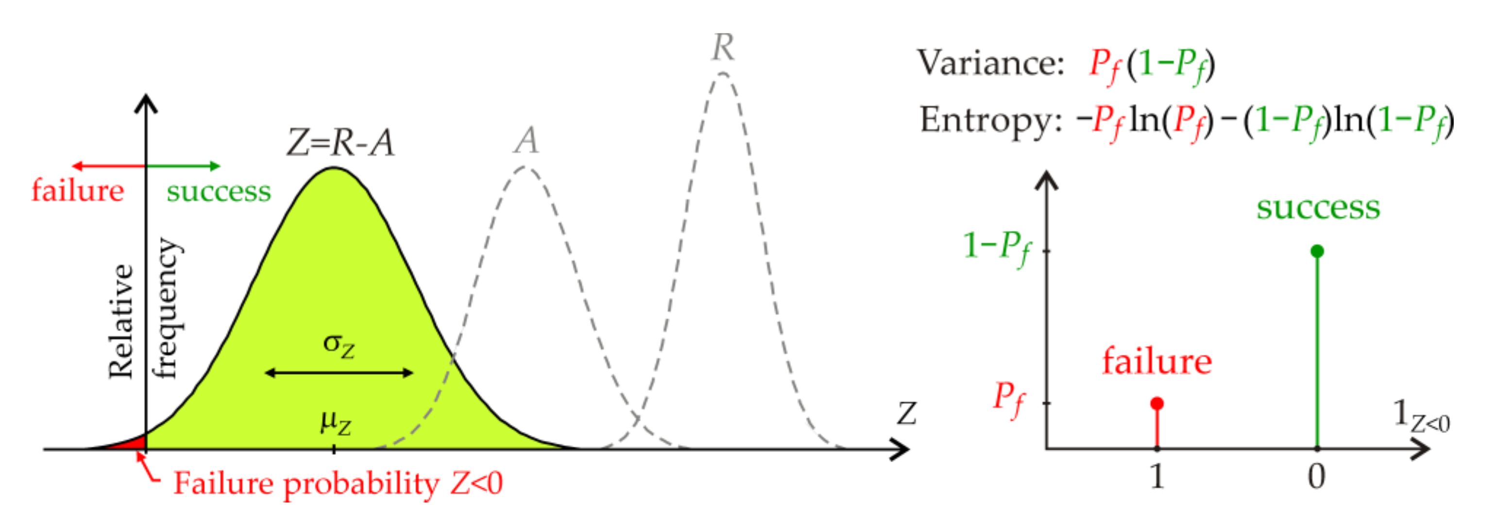
The basic condition of reliability can be written in the form of two random variables, load action A and resistance R; see Figure 1.

$$Z=R-A\ge 0.$$

(15)

In the limit state, a structure is reliable if Z ≥ 0 (R ≥ A), otherwise failure occurs. The resistance R and the load action A are two statistically independent variables that can be products of other random variables. The resistance R is often a function of the material strength and structural geometry [70,71], but it can also be limited by excessive deformations [72,73] or the sizes of fatigue cracks [74,75] and many other possible failure modes of different limit states [68,76].

Reliability is usually expressed in probabilistic terms [35]. The probability of failure P_f can be defined as the overload probability that A > R.

$$P_f=P\left(Z<0\right)=P\left(A>R\right).$$

(16)

The conventional measure of reliability is 1 − P_f. In engineering tasks, P_f is usually a small value that must be lower than the target failure probability when reliability is of interest [35]. Although P_f is an engineering characteristic, from a mathematical point of view it can be described as any other probability using the probability theory, where P_f can be described numerically using the number of desired outcomes divided by the total number of all outcomes. The concept of the SA of P_f presented in this article generally assumes P_f ∈ [0, 1].

Sensitivity measures based on the failure probability P_f as a dimensionless quantity are suitable for the analysis of structural reliability. The sensitivity measure oriented to P_f is defined as the average difference between the unconditional P_f and the conditional P_f|X_i on the input variable X_i. The article aims to study the effects of input variables on P_f using new types of sensitivity measures.

3.1. Sensitivity Measure Subordinated to Contrast

The generalization of Sobol sensitivity indices using sensitivity measures other than variance of model output was presented by Fort et al. [13]. Fort et al. [13] replaced variance with a contrast function that can be oriented to both variance (Sobol) and quantile or probability. Sensitivity indices are non-negative, and the sum of all indices is equal to one, as in the Sobol SA.

The first sensitivity measure oriented to probability is derived using the concept [13], where the minimum of the contrast function ψ(θ) can be written as:

$$\underset{\theta }{\min }\mathsf{\psi }\left(\theta \right)=\underset{\theta }{\min }E\left(\psi \left(Z,\theta \right)\right)=\underset{\theta }{\min }E{\left(1_{Z<0}-\theta \right)}^2=V\left(1_{Z<0}\right),$$

(17)

where indicator 1_Z<0 is a binary random variable with Bernoulli distribution. 1_Z<0 takes 1 with probability P_f and 0 with probability 1 − P_f. Equation (17) reaches a minimum if θ = P_f. Using variance V [1_Z<0], the Sobol-Hoeffding decomposition [14,64] can be followed, which leads to global reliability-oriented sensitivity indices [11,12,13].

Equations (6)–(8) can be rewritten by substituting Y = 1_Z<0 using Bernoulli distribution as follows:

$$f_0=E\left(1_{Z<0}\right)=P_f,$$

(18)

$$f_i\left(X_i\right)=E\left(1_{Z<0}\left|X_i\right.\right)-f_0=P_f\left|X_i\right.-P_f,$$

(19)

$$f_{ij}\left(X_i,X_j\right)=E\left(1_{Z<0}\left|X_i\right.,\hspace{0.33em}{X}_j\right)-f_i-f_j-f_0=P_f\left|X_i\right.,\hspace{0.33em}{X}_j-f_i-f_j-P_f.$$

(20)

Substituting Y = 1_Z<0 into Equation (9) we obtain:

$$V\left(1_{Z<0}\right)={\displaystyle \sum _{i}V\left(E\left(1_{Z<0}\left|X_i\right.\right) \right)}+{\displaystyle \sum _i{\displaystyle \sum _{j>i}V\left(E\left(1_{Z<0}\left|X_i\right.,X_j\right)\right)}}+\dots +V\left(1_{Z<0}\left|X_1,X_2,\dots ,X_M\right.\right).$$

(21)

The first-order sensitivity index can be written using Equation (21) as:

$${}^C{P}_i=\frac{V\left(E\left(1_{Z<0}\left|X_i\right.\right) \right)}{V\left(1_{Z<0}\right)}=\frac{V\left(1_{Z<0}\right)-E\left(V\left(1_{Z<0}\left|X_i\right.\right) \right)}{V\left(1_{Z<0}\right)}=\frac{P_f\left(1-P_f\right)-E\left(P_f\left|X_i\right.\left(1-P_f\left|X_i\right.\right)\right)}{P_f\left(1-P_f\right)},$$

(22)

where V[1_Z<0] = P_f (1 − P_f) is the variance of the Bernoulli distribution. Equations (18)–(22) are a review of the previous work [12] and therefore have the same definition as [12]. For direct use in the Sobol SA, one can write Y = 1_Z<0 = (|Z|−Z)/(2Z).

Fixing X_i directly influences P_f; hence, the sensitivity index ^CP_i is reliability-oriented. The sensitivity index ^CP_i measures the average influence of X_i on P_f using a sensitivity measure that can be written as follows:

$${}^{C}M\left(P_f\right)=P_f\left(1-P_f\right),$$

(23)

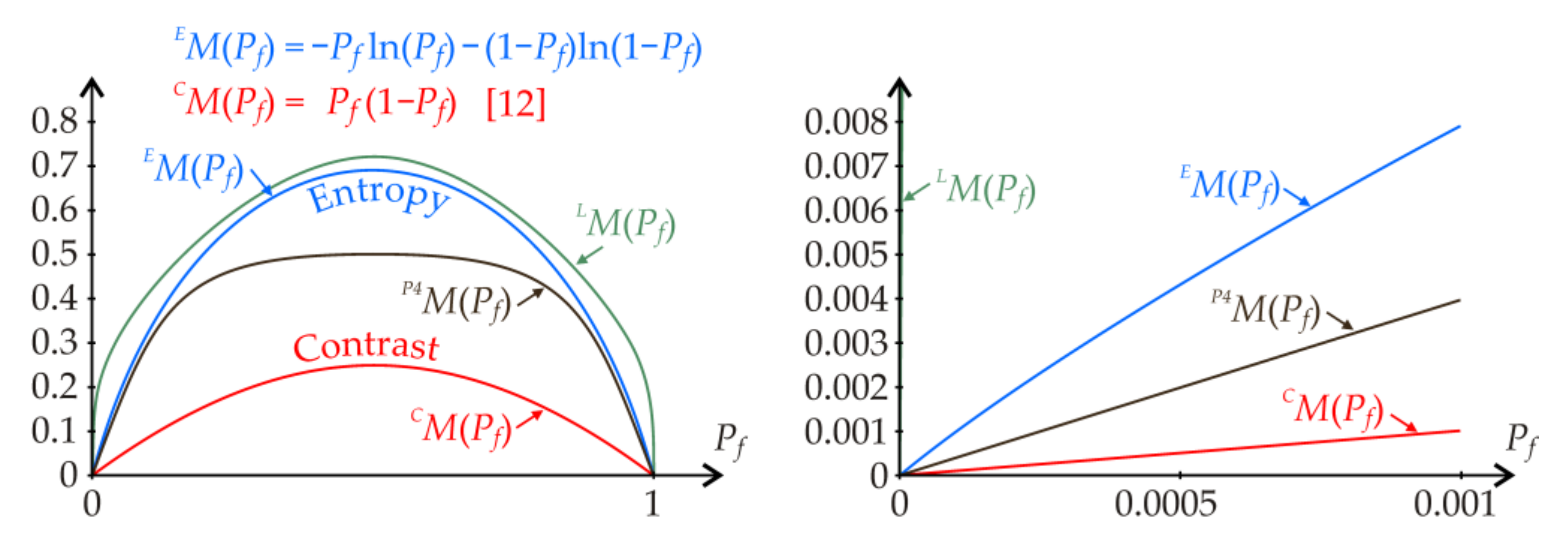
where P_f is the output of the stochastic computational model. Function P_f (1 − P_f) has the shape of a symmetrical dome with a maximum value for P_f = 0.5 and two minima for P_f = 0 and P_f = 1; see Figure 2.

The sensitivity measure ^CM(P_f) reaches zero when all the input variables are fixed. The sensitivity measure ^CM(P_f) after Sobol leads to sensitivity indices with the sum of all the indices equal to one, but with a significantly higher proportion of higher-order sensitivity indices than the classical Sobol SA of model output; see numerical studies [19].

One may ask whether the variance V[1_Z<0] is the only consistent measure of uncertainty. It can be shown that other sensitivity measures are possible. The sensitivity measure ^CM(P_f) in the shape of a dome indicates that the sensitivity measure ^CM(P_f) can be approximated by other suitable dome-shaped functions.

3.2. Sensitivity Measure Based on Entropy

A new probability-oriented sensitivity measure can be written using Shannon’s discrete entropy [77]. The entropy of discrete probabilities can be defined using the formula:

$$H\left(Z\right)=-{\displaystyle \sum _{i=1}^{n}P\left(z_i\right)\cdot {\log }_b\left(P\left(z_i\right)\right)}.$$

(24)

One may ask: why is entropy a good measure of uncertainty at all? Few mathematical constructs have the desired basic properties: uncertainty is an additive for independent events; adding an outcome with zero probability has no effect, and the measure of uncertainty is continuous in all its arguments; see, e.g., [78,79].

Distribution-oriented SA based on discrete entropy [80] is known but has never been presented in the context of the ROSA of P_f. The subject of interest of the ROSA is only P_f, not the entire distribution Z. To this end, the distribution Z is replaced by a two-probability mass function; see Figure 1.

Equation (24) can be rewritten in the form of a sensitivity measure

$${}^{E}M\left(P_f\right)=H\left(1_{Z<0}\right)=-P_f\cdot {\log }_b\left(P_f\right)-\left(1-P_f\right)\cdot {\log }_b\left(1-P_f\right)=-{\log }_b\left(P_f{}^{P_f}{\left(1-P_f\right)}^{1-P_f}\right),$$

(25)

based on the discrete entropy of a two-probability mass function; see Figure 1. Entropy (the degree of surprise) is zero if it is certain that one particular event will occur; therefore, the entropy of a deterministic quantity is zero similar to zero variance. The base of the logarithm b in Equation (25) influences only the size of the amplitude of the symmetrical dome-shaped function ^EM(P_f) but does not change its shape.

Discrete entropy lacks some useful properties of variance. For example, the equality V(E(1_Z<0|X_i)) = V(1_Z<0) − E(V(1_Z<0|X_i)) generally does not apply in H(E(1_Z<0|X_i)) ≠ H(1_Z<0) − E(H(1_Z<0|X_i)). Nevertheless, a useful sensitivity measure is the form H(1_Z<0) − E(H(1_Z<0|X_i)) with which it is possible to go back to the path of Sobol’s decomposition; see Equations (21) and (22), etc.

Both sensitivity measures, ^EM(P_f) and ^CM(P_f), are symmetrical and dome-shaped but have slightly different shapes.

3.3. Sensitivity Measure Based on Other Functionals

Further approximations of the sensitivity measure ^CM(P_f) are presented to study the influence of dome shapes on the SA results. The goal is to observe changes in the sensitivity indices using four variants of sensitivity measures in the case studies. The effect of the sensitivity measure on the sensitivity indices can be significant, as will be shown.

Equation (23) can be rewritten into a form that allows the formulation of a new sensitivity measure:

$${}^{C}M\left(P_f\right)=P_f\left(1-P_f\right)=0.5-\frac{{\left(2P_f-1\right)}^2}{2}.$$

(26)

Equation (26) can be rewritten using parabolas of other degrees as:

$${}^{Pa}M\left(P_f\right)=0.5-\frac{{\left|2P_f-1\right|}^a}{2},$$

(27)

where a > 0. Similarly, other dome-shaped sensitivity measures can be formulated; for example:

$${}^{L}M\left(P_f\right)=\frac{1}{-{\log }_b\left(P_f\cdot \left(1-P_f\right)\right)},$$

(28)

where the base of the logarithm b changes the size of the amplitude (measure) of the dome-shaped function but does not change its shape.

3.4. Probability-Oriented Sensitivity Indices

The first-order P_f oriented sensitivity index based on sensitivity measure M(P_f) = {^CM(P_f), ^EM(P_f), ^PaM(P_f), ^LM(P_f)} can be written as:

$$P_i=\frac{M\left(P_f\right)-E\left(M\left(P_f\left|X_i\right.\right)\right)}{M\left(P_f\right)}.$$

(29)

The influence quantified by P_i can be referred to as the main effect. The second-order P_f oriented sensitivity index is written analogously:

$$P_{ij}=\frac{M\left(P_f\right)-E\left(M\left(P_f\left|X_i\right.,X_j\right)\right)}{M\left(P_f\right)}-P_i-P_j.$$

(30)

The third-order P_f oriented sensitivity index is written analogously:

$$P_{ijk}=\frac{M\left(P_f\right)-E\left(M\left(P_f\left|X_i\right.,X_j,X_k\right)\right)}{M\left(P_f\right)}-P_i-P_j-P_k-P_{ij}-P_{ik}-P_{jk}.$$

(31)

Similarly, other P_f oriented sensitivity indices, which quantify higher-order interactions, can be written. In Equations (29)–(31), E(M(•)) cascades down as the number of fixed input variables increases until it reaches zero when all the variables are fixed.

Regarding the contrast in Equation (23), each sensitivity index is non-negative and the sum of all the sensitivity indices is equal to one; see Equation (32). Regarding the alternative sensitivity measures, it is obvious to see that the sum is equal to one.

$${\displaystyle \sum _i{P}_i}+{\displaystyle \sum _i{\displaystyle \sum _{j>i}{P}_{ij}}}+{\displaystyle \sum _i{\displaystyle \sum _{j>i}{\displaystyle \sum _{k>j}{P}_{ijk}}}}+\dots +P_{123\dots M}=1.$$

(32)

However, it is questionable whether each sensitivity index is always non-negative when using the three types of newly proposed alternative sensitivity measures in Equations (25), (27) and (28). The reason for the negative indices is the negative terms in Equations (29)–(31). Higher-order sensitivity indices can be negative due to the relatively high lower-order sensitivity indices that are subtracted in the equations. A conservative view means not wanting negative sensitivity indices, similar to the Sobol SA. However, negative sensitivity indices may not be a phenomenon that invalidates the results. If the index has a negative value, the way it is ranked compared to the other indices does not change. A smaller index means less influence, a higher index means more influence, regardless of the sign. From this point of view, negative indices are permissible. Allowing negative indices in Equation (32) means abandoning conservative views based on the non-negative sensitive indices of the classical types of SA, such as [15,43].

Although the non-negativity of each index is observed in the case studies, it has not yet been mathematically proven. It would be convincing if this property could be mathematically better explained.

For example, for two input random variables it can be shown that P₁ + P₂ + P₁₂ = 1, because E(M(1_Z<0|X₁, X₂) = 0 at the edges of the dome. The total number of sensitivity indices is 2^M − 1. It follows from the concept of calculating sensitivity indices that each sensitivity measure can be multiplied by an arbitrary positive constant without influencing the values of the sensitivity indices. In practice, this means that the amplitudes of the dome-shaped measures do not matter; see Figure 2. With this justification, the natural logarithm is applied to the sensitivity measures ^EM(P_f) and ^LM(P_f) throughout the article.

The sensitivity ranking can be evaluated using total indices P_Ti, the significance of which is analogous to P_Ti, but with an orientation to P_f.

$$P_{Ti}=\frac{E\left(M\left(P_f\left|X_{~i}\right.\right)\right)}{M\left(P_f\right)}.$$

(33)

Index P_Ti can be calculated as the sum of the indices of all orders with index i similar to Sobol’s SA application [6]. For example, for the two input variables X₁ and X₂, we have P_T1 = P₁ + P₁₂ and P_T2 = P₂ + P₁₂. The sensitivity ranking is determined by comparing P_T1 and P_T2.

4. Case Study with Two Input Variables

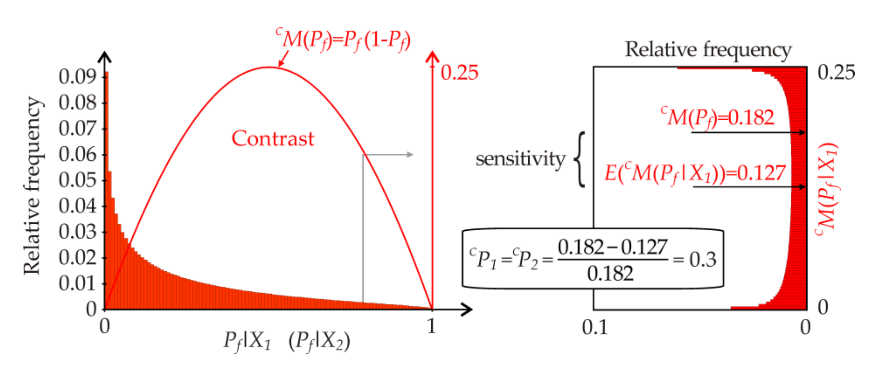
The first study describes the methodology for calculating sensitivity indices in the case of two input random variables R ~ N(2, 1) and A ~ N(1, 1), where Z = R − A and Z ~ N(1, 2); P(Z<0) = 0.24; and ^CM(0.24) = 0.24(1 − 0.24) = 0.182. Let R be X₁ and A be X₂. The subject of interest of the Sobol SA is the variance of Z. If P_f is the subject of interest, a dome-shaped sensitivity measure M(P_f) is used instead of the variance; see Figure 2.

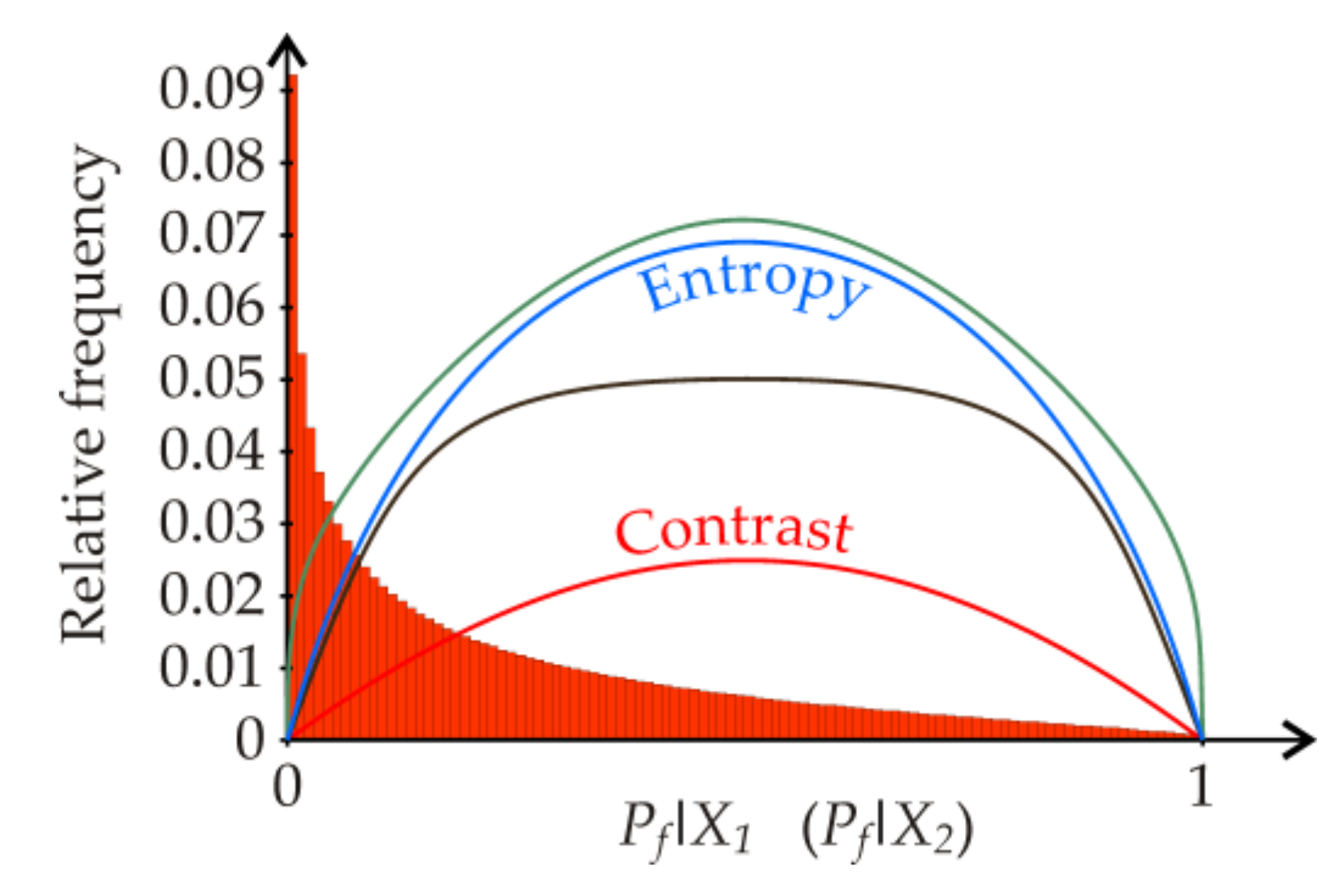
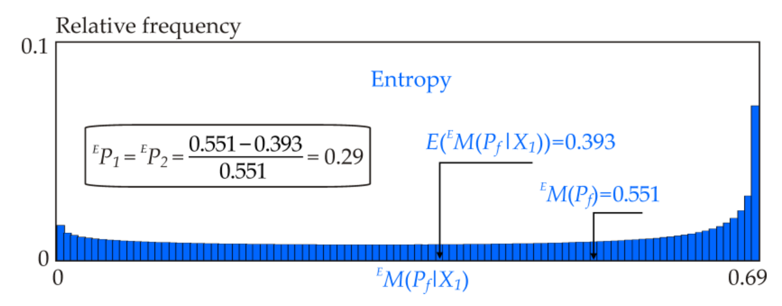
X₁ is sampled using one hundred thousand runs of the LHS method [81,82]. For the LHS realization of x₁, the realization of P_f|x₁ is calculated by numerical integration according to Simpson’s rule from Z ~ N(x₁ − 1, 1). The distribution of one hundred thousand random realizations of P_f|X₁ is plotted in a histogram; see Figure 3. The histogram P_f|X₂ is the same as the histogram P_f|X₁, therefore it is not plotted separately. The explanation applies to both of the random variables, X₁ and X₂.

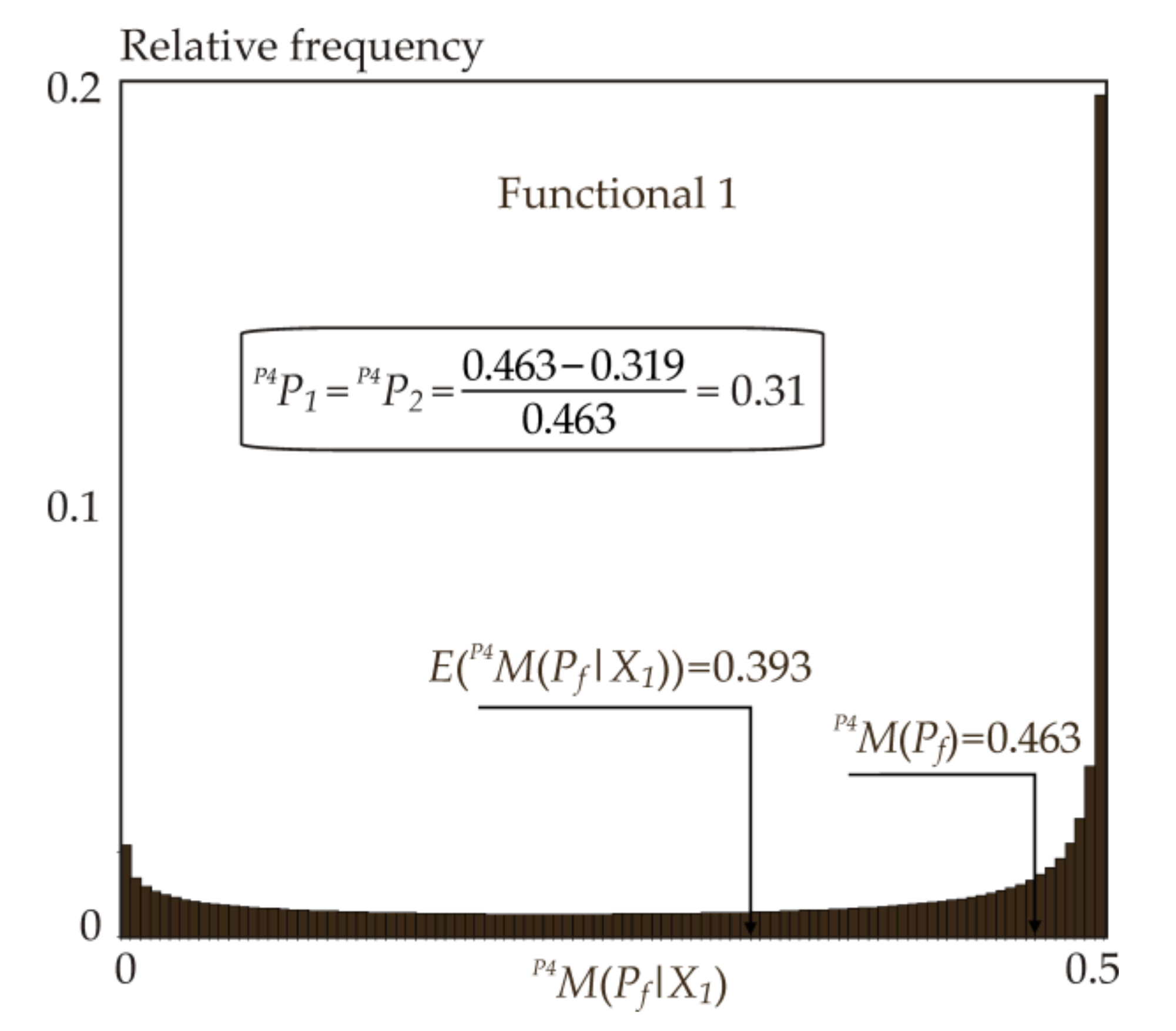
The dome transforms the histogram P_f|X₁ into the histogram of the sensitivity measure M(P_f|X₁). Histogram M(P_f|X₁) differs according to the shape of the dome used; see Figure 4, Figure 5, Figure 6 and Figure 7. The further the sample x₁ moves away from the median X₂, the more the sensitivity measure M(P_f|x₁) decreases and the greater the influence of x₁ on P_f. The influence of sample x₁ on P_f is maximum if M(P_f|x₁) → 0 if P_f|x₁ → 0 or P_f|x₁ → 1. The influence of sample x₁ on P_f is zero if P_f|x_1=0.3 = 0.24. The influence of X₁ on P_f using the entire population E(M(P_f|X₁)) is evaluated according to Equation (29) where P₁ ∈ [0, 1]. The sensitivity index P₂ is evaluated analogously. The values of the first-order sensitivity indices are shown in Figure 4, Figure 5, Figure 6 and Figure 7.

In order for the sum of all the indices to be equal to one, the methodology for calculating the sensitivity index of the last (here second) order is important. If X₁ and X₂ are fixed (deterministic) variables, then P_f can only be 0 or 1. The sum of all the indices must be equal to one. Therefore, the sum of all indices of order which is lower than the last is subtracted from one, where (M(P_f) − 0)/M(P_f)) = 1. Zero in the numerator is the product of the edges of the dome, M(0) = 0 or M(1) = 0; see Figure 2. Entropy, variance, and other measures are equal to zero. Then, it is possible to write P₁₂ = 1 − P₁ − P₂ and thus P₁ + P₂ + P₁₂ = 1.

In this case study, the numerical results of the second-order sensitivity indices from all the sensitivity measures are ^CP₁₂ = 0.4, ^EP₁₂ = 0.42, ^P4P₁₂ = 0.38, and ^LP₁₂ = 0.62.

5. Case Study with Five Input Variables

The second case study illustrates the SA of P_f using five input random variables. The case study compares the sensitivity indices computed using the four sensitivity measures ^CM(P_f), ^EM(P_f), ^P4M(P_f), and ^LM(P_f).

The reliability of a steel bar subjected to tension is analyzed. The condition of reliability in Equation (15) is studied using five input random variables, where two variables are on the load side A and three variables are on the resistance side R.

5.1. Stochastic Model: Output and Input Random Variables

The load action A is the product of two other known loading distributions acting on the bar:

$$A=G+Q,$$

(34)

where G is the permanent load action and Q is the long-term leading single variable load action. According to EN1990 [35], G can be considered with the Gauss pdf and Q with the Gumbel-max pdf [83]; see

Table 1. The load action A—input random variables.

Characteristic	Index	Symbol	Pdf	Mean Value μ	Standard Deviation σ
Permanent load	1	G	Gauss	165.3 kN + 0.5μF	16.5 kN
Variable load	2	Q	Gumbel-max	17.51 kN + 0.5μF	6.2 kN

.

Where μ_F is a parameter which is considered using three values −13.58 kN, 0 kN, and 13.37 kN.

The resistance R of a steel drawn bar made of steel of grade S235 is analyzed. The statistical characteristics of the yield strength and the geometric characteristics of the rectangular cross-section are taken from experimental research [84]; see

Table 2. The resistance R—input random variables.

Characteristic	Index	Symbol	Pdf	Mean Value μ	Standard Deviation σ
Yield strength	3	fy	Gauss	297.3 MPa	16.8 MPa
Section thickness	4	t2	Gauss	12 mm	0.55 mm
Section width	5	b	Gauss	80 mm	0.79 mm

.

All the inputs are uncorrelated. The static resistance is a product of the thickness and width (cross-sectional area t₂·b) and the yield strength f_y:

$$R=b\cdot t_2\cdot f_y.$$

(35)

The formulae for calculating the mean value μ_R, the standard deviation σ_R, and the standard skewness a_R of R are given in [39,67]. The goodness-of-fit tests and comparative studies [83] have confirmed that the probability density distributions of R can be approximated very accurately using a three-parameter lognormal pdf.

Failure occurs when A > R. In Equation (16), P_f is estimated using numerical integration according to Simpson’s rule using more than ten thousand integration steps [83]. The inequality A > R is treated as Q > R − G, where Q has a Gumbel-max pdf and R − G is approximated by a three-parameter lognormal pdf. A detailed description of the numerical integration algorithm, including comparative studies demonstrating the high accuracy of the P_f estimation, is published in [83].

The parameter μ_F = {−13.58 kN, 0 kN, 13.37 kN} is chosen to lead to P_f = {8.5 × 10⁻⁶, 7.2 × 10⁻⁵, 4.8 × 10⁻⁴}, which are the basic design cases listed in standard EN1990 [35]; see

Table 3. The target values of failure probability P_f according to [35].

Reliability Class	Pf
RC3	8.5 × 10−6
RC2	7.2 × 10−5
RC1	4.8 × 10−4

.

5.2. The Sensitivity Analysis Results

Estimates of sensitivity indices are obtained using numerical integration.

In Equation (29), the first-order indices P_i are estimated using double-nested-loop computation [34]. In the inner loop, the estimate of P_f|X_i = P((Z|X_i) < 0) is computed using the procedure described in the previous chapter and [83]. In the outer loop, E[•] is computed by numerical integration of the pdf of X_i with a small step Δx_i taken over [μ_Xi − 12σ_Xi, μ_Xi + 12σ_Xi].

In Equation (30), the second-order indices P_ij are estimated using three-nested-loop computation. In the inner loop, the estimate of P_f|X_i, X_j = P((Z|X_i) < 0) is computed using the procedure described in the previous chapter; see also [83]. In the two outer loops, E[•] is computed by double numerical integration of the joint pdf of X_i, X_j with a small step Δx_i taken over [μ_Xi − 12σ_Xi, μ_Xi + 12σ_Xi] and a small step Δx_j taken over [μ_Xj − 12σ_Xj, μ_Xj + 12σ_Xj].

The third- and fourth-order indices are computed analogously. The third-order index requires a triple numerical integral, and the fourth-order index requires a quadruple numerical integral. The fifth-order index completes the sum of all the lower-order indices to one.

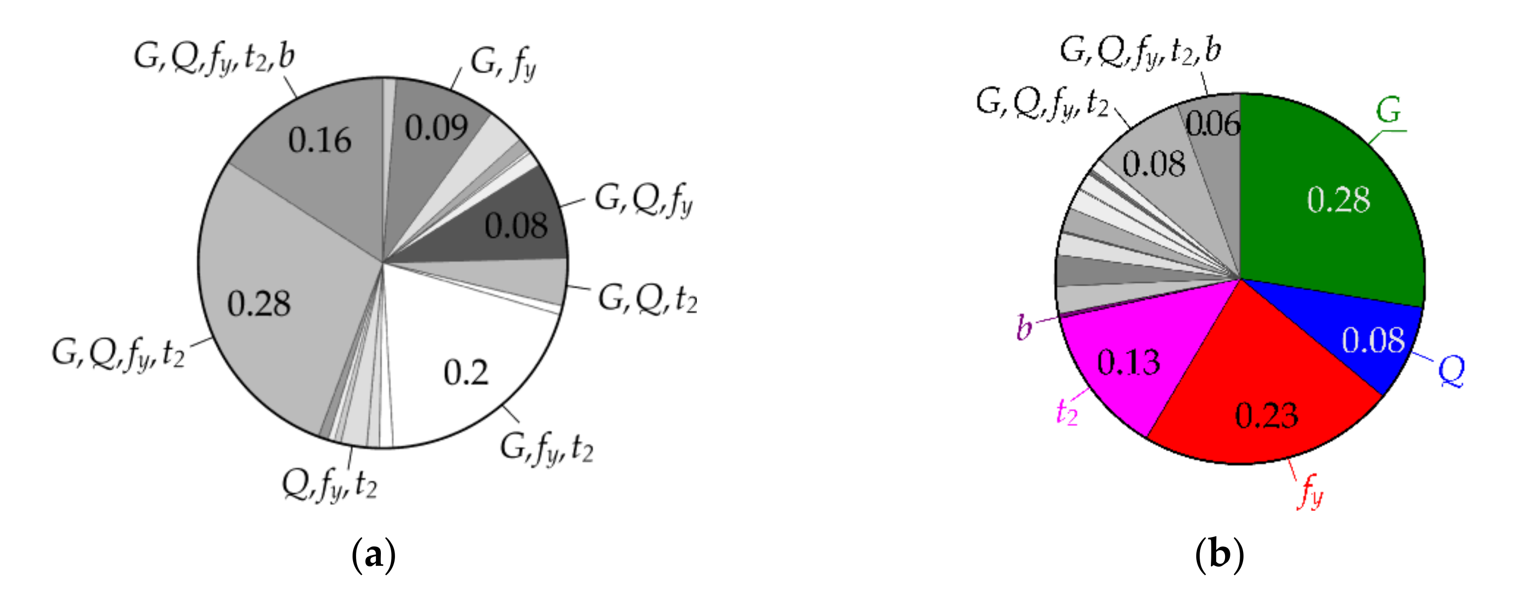
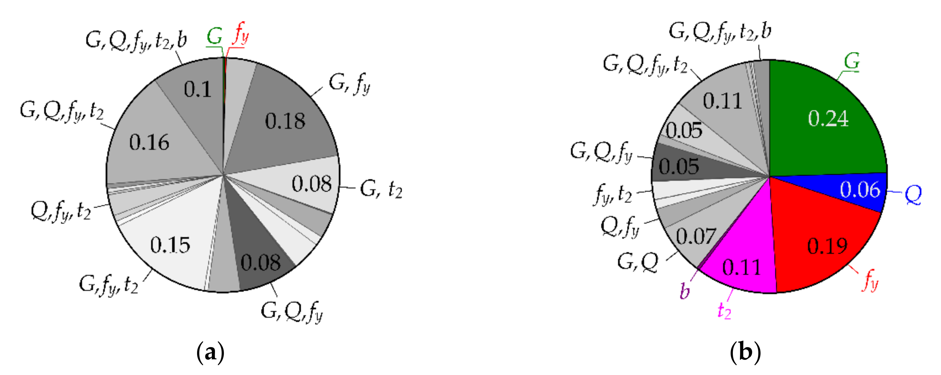
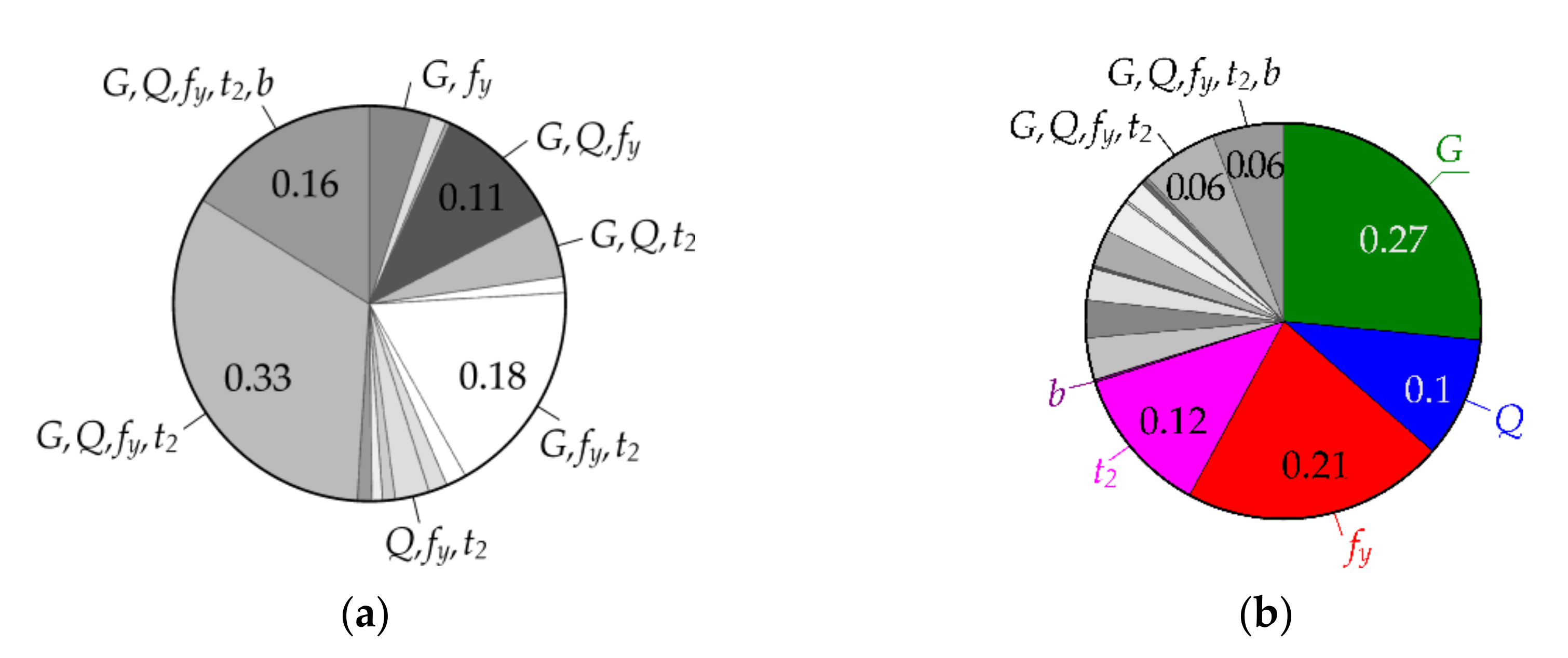
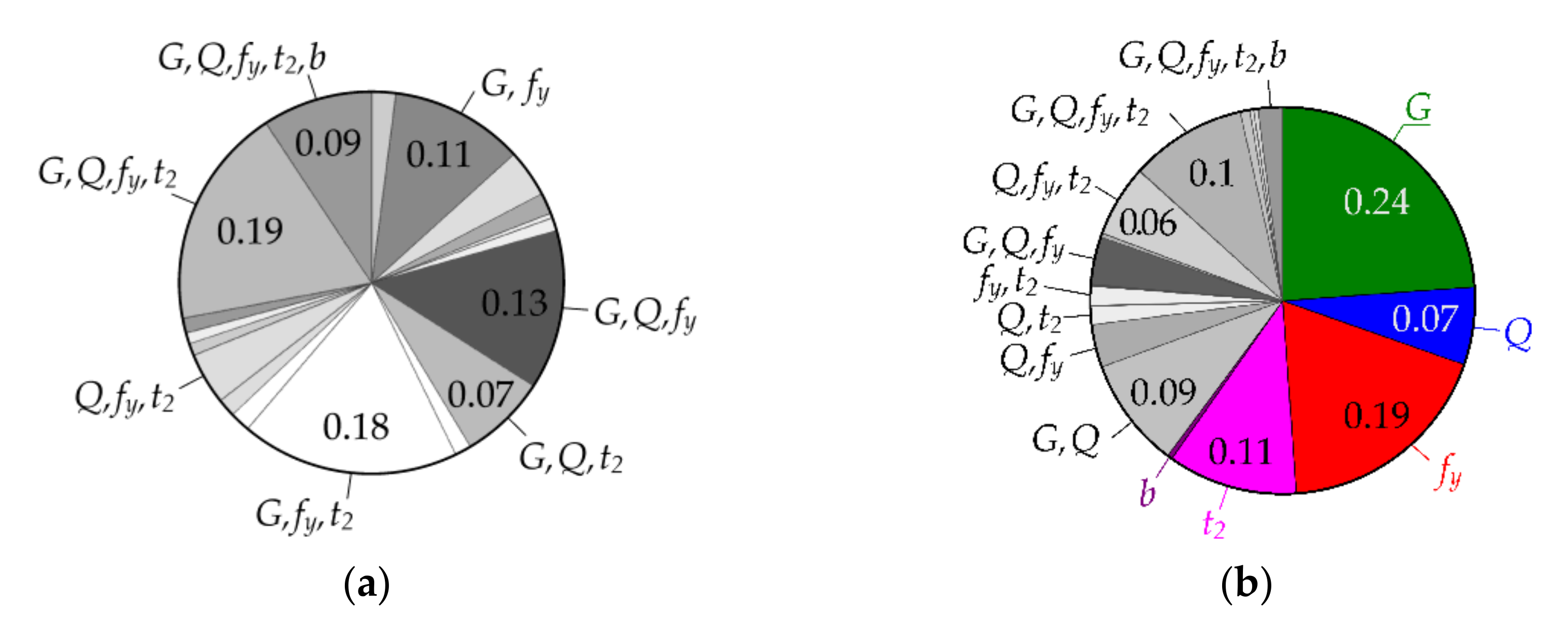
The sensitivity indices computed using the sensitivity measures ^CM(P_f), ^EM(P_f), ^P4M(P_f), and ^LM(P_f) are plotted in Figure 8, Figure 9, Figure 10 and Figure 11.

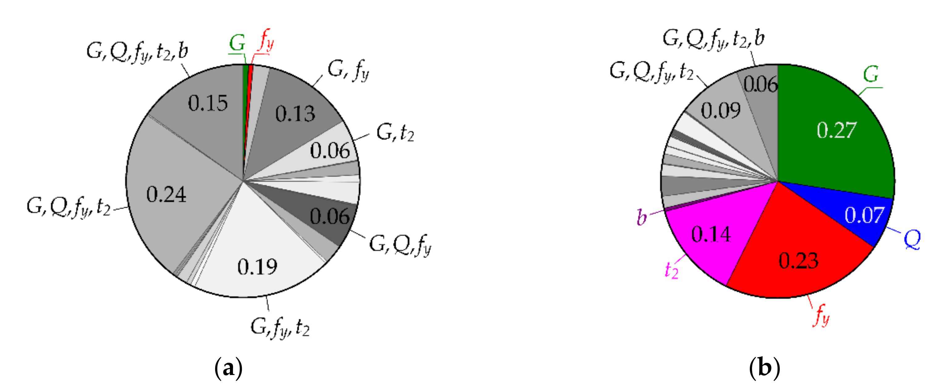
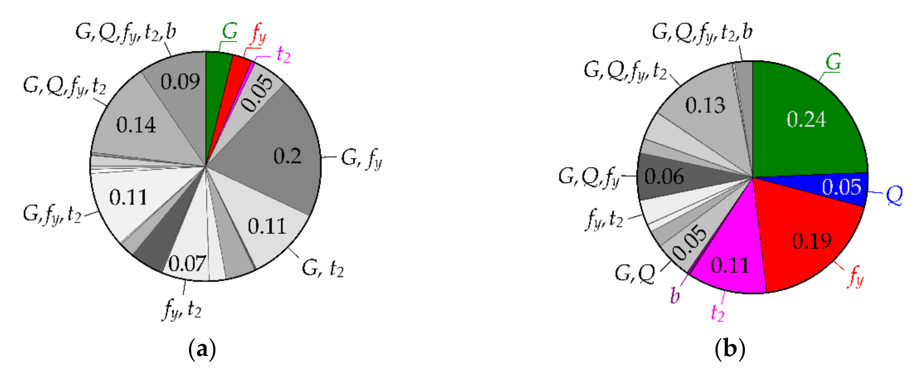
Figure 8, Figure 9, Figure 10, Figure 11, Figure 12 and Figure 13 contain a lot of information, such as the main and interaction effects of the five input variables varying between the four kinds of measures and the three levels of P_f. The sum of the main effects ∑P_i (colored regions) vary from 0 (contrast approach, P_f = 8.5 × 10⁻⁶) to 0.72 (entropy approach, P_f = 7.2 × 10⁻⁵). On the other hand, the interaction effects 1 − ∑P_i (grey regions) vary from 0.28 (entropy approach, P_f = 7.2 × 10⁻⁵) to 1 (contrast approach, P_f = 8.5 × 10⁻⁶). The pie charts on the left have the measures ^CM(P_f) and ^P4M(P_f) based on second-degree and fourth-degree parabolas, which give a very small proportion of the first-order indices. The pie charts on the right have the measures ^EM(P_f) and ^LM(P_f) based on logarithms, which give more than a sixty-percent share of the first-order indices. The colored pie charts on the right are similar to each other. The colored pie charts on the left are less similar to each other. The measure ^LM(P_f) leads to a very small proportion of the last-order sensitivity index compared to ^CM(P_f). The origin of these phenomena is not yet sufficiently understood at this stage and requires further analysis.

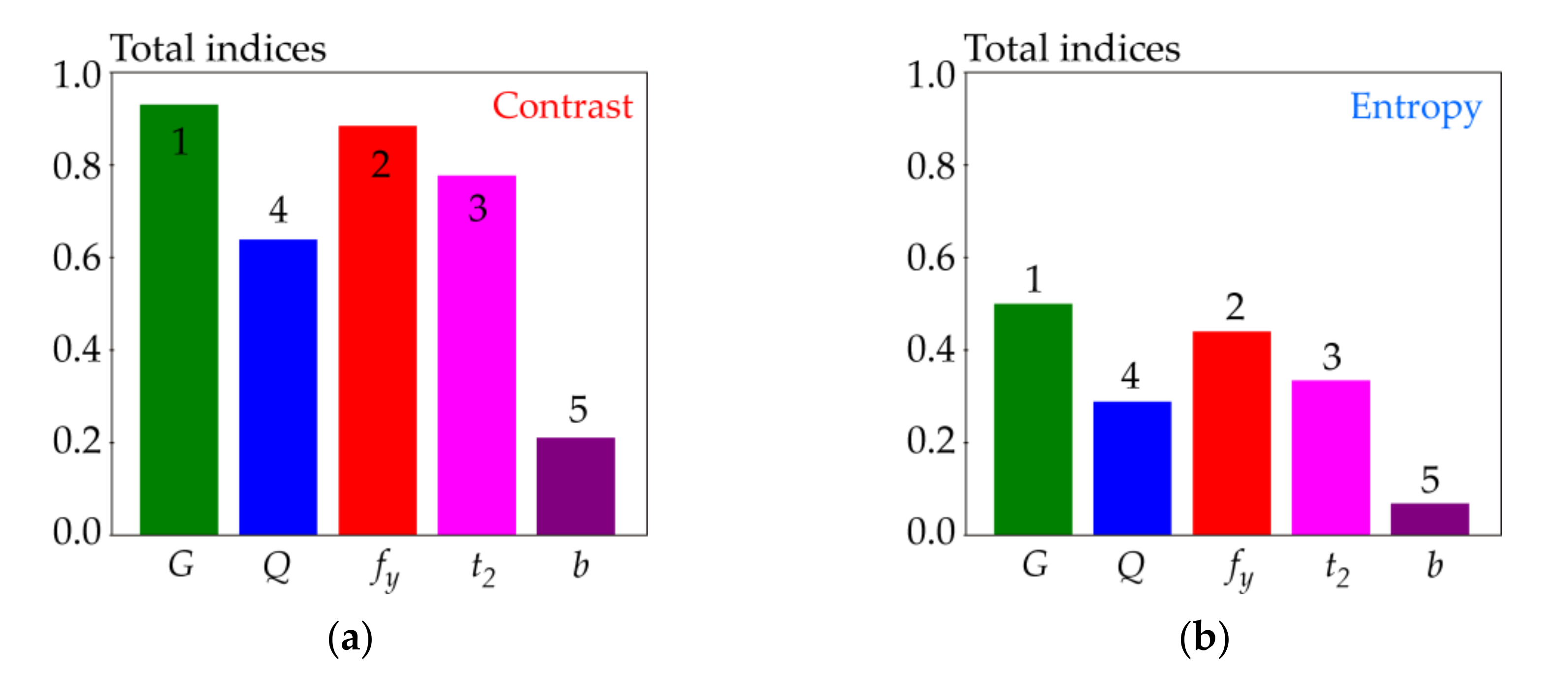
Identifying the sensitivity ranking of input variables using all sensitivity indices is all the more difficult the more the input variables and interaction effects. The sensitivity ranking can be effectively evaluated using the total indices. As all three target values of failure probability P_f have approximately the same total indices, only SA of P_f = 7.2 × 10⁻⁵ is shown; see Figure 14 and Figure 15.

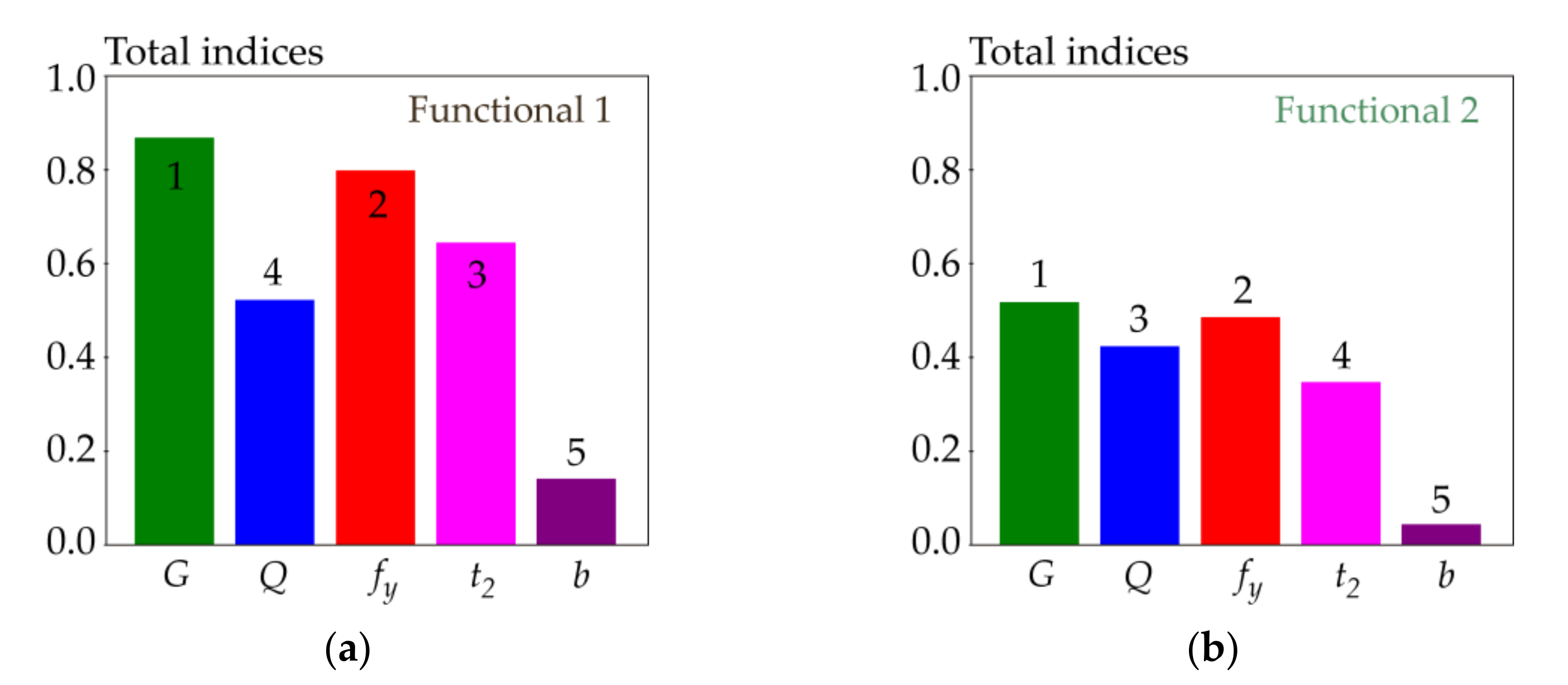
The total indices evaluated using the sensitivity measures ^CM(P_f), ^EM(P_f), and ^P4M(P_f) determined the sensitivity of the input variables to P_f in descending order as G, f_y, t₂, Q, b. The sensitivity measure ^LM(P_f) identified a different sensitivity ranking G, f_y, Q, t₂, b, which differs in the third and fourth place, but the identification of the non-influential b and the dominant G, f_y variables is the same.

A simple verification of results can be performed. Let us fix one input variable at the mean value and observe the effect on P_f. The failure probability without any fixation is P_f = 7.2 × 10⁻⁵ (μ_F = 0). The values of P_f obtained upon fixation are 1.17 × 10⁻⁶, 3.67 × 10⁻⁵, 3.82×10⁻⁶, 1.5 × 10⁻⁵, and 6.86 × 10⁻⁵. The smallest value of 1.17 × 10⁻⁶ means the greatest influence of G on P_f. The sensitivity ranking G, f_y, t₂, Q, b shows that the results are as presented above (realistic).

The Sobol SA of Z leads to the sensitivity indices S₁ = 0.363, S₂ = 0.051, S₃ = 0.346, S₄ = 0.228, and S₅ = 0.011, which are computed analytically [39,67]. The calculation of the higher-order Sobol indices or the total indices is not necessary because the sum of the first-order indices is not far from one: S₁ + S₂ + S₃ + S₄ + S₅ ≈ 1. This is a significant difference compared to the results from ^CM(P_f) and ^P4M(P_f). The sensitivity ranking G, f_y, t₂, Q, b determined using the five first-order Sobol sensitivity indices is the same as that determined by the ROSA of P_f using 31 indices. The advantage of the Sobol SA is the lower computational costs. Although the Sobol SA is not reliability-oriented, it is empathetic to reliability.

6. Discussion

The subject of this article is the global SA of a one-bit variable 1_Z<0 with Bernoulli distribution, where failure occurs with probability P_f. New alternative sensitivity measures ^EM(P_f), ^P4M(P_f), and ^LM(P_f) are formulated by approximating the variance V(1_Z<0) = P_f(1 − P_f) using entropy and other dome-shaped functions; see Figure 2.

The first case study presents a reliability design condition with two input random variables with the Gauss pdf [35]. All the presented sensitivity measures ^CM(P_f), ^EM(P_f), ^P4M(P_f), and ^LM(P_f) lead to sensitivity indices with good structure. The “good structure” means that the sensitivity indices are non-negative and their sum is equal to 1.

In the second case study, all the presented sensitivity measures provide a good structure of sensitivity indices. It is shown that the shape of the dome affects both the value of the sensitivity indices (significant influence) and the sensitivity ranking of the input variables (little influence). The sensitivity measures ^CM(P_f) and ^P4M(P_f) give an extremely high proportion of higher-order sensitivity indices; see the grey areas in the left parts of Figure 8 to Figure 13. In contrast, the sensitivity measures ^EM(P_f) and ^LM(P_f) give a pleasantly high proportion of first-order sensitivity indices; see the colored regions in the right parts of Figure 8, Figure 9, Figure 10, Figure 11, Figure 12 and Figure 13. Other sensitivity measures can be examined; for example, sin(π·P_f) gives sensitivity indices reminiscent of the contrast approach. The use of total indices to determine the sensitivity ranking is appropriate in all cases.

A certain degree of empiricism and data collection was used in the discovery of the sensitivity measures. Not every dome-shaped sensitivity measure works well in all numerical studies. For example, the introduction of a sensitivity measure in the shape of a semicircle (P_f(1 − P_f))^0.5 does not give a good structure of sensitivity indices for an SA of P_f = 7.2 × 10⁻⁵ (the sum of first-order indices is 1.62 > 1 and some higher-order indices are even negative); however, if P_f = 0.4, then a good structure of indices is obtained. From a numerical point of view, when P_f approaches zero, the direction of the tangent of the semicircle approaches infinity, which makes it difficult to measure changes in very small P_f.

Only variance V[1_{Z < 0}] strictly follows the Sobol-Hoeffding decomposition [14,64,65] by using ^CM(P_f) = P_f(1 − P_f), because contrast sensitivity indices are a special type of Sobol sensitivity indices [12]. Although the alternative sensitivity measures ^EM(P_f), ^P4M(P_f), and ^LM(P_f) always gave non-negative sensitivity indices and no other behavior was observed, general evidence has not been presented. From an engineering point of view, all the presented sensitivity measures ^CM(P_f), ^EM(P_f), ^P4M(P_f), and ^LM(P_f) can be recommended, but with the condition of checking the good structure of the sensitivity indices for alternative measures ^EM(P_f), ^P4M(P_f), and ^LM(P_f).

Preliminary studies suggest that a good structure of the sensitivity indices can also be obtained for non-linear function R with buckling [57,85], lateral-torsional buckling [86], or their interactions [87,88]. The concept of the SA of P_f can be applied to the probabilistic analysis of reliability where design reliability conditions prevail [35], with the assumption that R and A are Gauss pdf and P_f is low [89].

The studies presented here have shown that the sensitivity measure does not influence the identification of the input variables with the greatest and least influence, which is consistent with the conclusions of other types of SA; see, e.g., [38,39]. The results of the SA can be applied to the optimization of reliability-oriented stochastic models, where input variables with a small influence on P_f can be considered deterministic. On the contrary, input variables with strong influence must have statistical characteristics and a pdf shape determined with increased precision.

The dominant variables can be further studied using other types of SA if the first moments [70], or the pdf shapes [90,91], or the importance of the components [92] are not explicitly known, as is often the case in engineering practice. Conversely, non-influential inputs can be fixed at any value of their domain without affecting P_f, usually close to the mean value.

For more complex structures, resistance R can be analyzed using the finite element method (FEM); see, e.g., [70,71]. In general, P_f can be estimated using the Monte Carlo (MC) method in combination with the FEM, but the CPU time requirements can be extreme for small P_f. For example, the number of MC runs must be greater than ≈100/P_f to achieve a coefficient of variation of P_f less than 0.1. The estimation of a high number of sensitivity indices also increases the computational time due to the high dimensionality of the models. The computational limitations of the ROSA using a crude MC with a direct call to the numerical demanding model are substantial when the fixing of one or more input variables implies very small values of P_f. Advanced approximation modelling methods and improved MC methods with parallelizable algorithms may be the solution [93].

Further research should aim to use surrogate models to estimate small P_f from high-dimensional numerical models. Unfortunately, a characteristic feature of the ROSA results of small P_f is the high proportion of higher-order sensitivity indices; therefore, the surrogate models must capture most of the variation information contained in the original input. The presented sensitivity measure with a higher proportion of first-order sensitivity indices is offered as a possible solution to this problem.

There are many sensitivity measures that have not yet been discovered, which is proof that the theory is not complete. Alternative sensitivity measures may lead to non-negative and negative sensitivity indices with the sum of all the indices equal to one. If the index has a negative value, then its evaluation of ranking does not change compared to the other indices. This suggests that the occurrence of negative sensitivity indices may not be problematic. Further research on sensitivity measures would be useful.

7. Conclusions

The article presented new sensitivity measures in the global sensitivity analysis of failure probability P_f. The case studies compared sensitivity indices from all four sensitivity measures in application to small values of P_f. The sensitivity ranking of the input variables is approximately the same from each sensitivity measure, but the proportions of the main and interaction effects differ significantly. A common characteristic of the sensitivity measures is a symmetrical dome shape. The results are only affected by the shape of the dome and not its rise.

Sensitivity analysis subordinated to contrast has non-negative sensitivity indices with the sum of all the indices equal to one. These properties are inherited from Sobol but are also observed in the alternative sensitivity measures.

The alternative sensitivity measure can be viewed as a rough approximation of the dome-shaped function of the variance P_f(1 − P_f) of the contrast sensitivity measure. A good alternative to contrast is discrete entropy, which has variance-like properties but leads to significantly higher proportions of first-order sensitivity indices. The properties of the entropy and other sensitivity measures should be further studied.

References

- Derennes, P.; Morio, J.; Simatos, F. Simultaneous estimation of complementary moment independent and reliability-oriented sensitivity measures. Math. Comput. Simul. 2021, 182, 721–737. [Google Scholar] [CrossRef]
- Jebur, H.Q.; Al-Zaidee, S.R. Non-deterministic approach for reliability evaluation of steel portal frame. Civ. Eng. J. 2019, 5, 1684–1697. [Google Scholar] [CrossRef]
- Melchers, R.E. Structural Reliability Analysis and Prediction, 2nd ed.; John Wiley: Chichester, UK, 2002. [Google Scholar]
- Xiao, S.; Lu, Z. Structural reliability analysis using combined space partition technique and unscented transformation. J. Struct. Eng. 2016, 142, 04016089. [Google Scholar] [CrossRef]
- Cheng, K.; Lu, Z.; Xiao, S.; Lei, J. Estimation of small failure probability using generalized subset simulation. Mech. Syst. Signal Process. 2022, 163, 108114. [Google Scholar] [CrossRef]
- Saltelli, A.; Ratto, M.; Andres, T.; Campolongo, F.; Cariboni, J.; Gatelli, D.; Saisana, M.; Tarantola, S. Global Sensitivity Analysis: The Primer; John Wiley & Sons: West Sussex, UK, 2008. [Google Scholar]
- Cheng, K.; Lu, Z.; Ling, C.; Zhou, S. Surrogate-assisted global sensitivity analysis: An overview. Struct. Multidiscipl. Optim. 2020, 61, 1187–1213. [Google Scholar] [CrossRef]
- Javidan, M.M.; Kang, H.; Isobe, D.; Kim, J. Computationally efficient framework for probabilistic collapse analysis of structures under extreme actions. Eng. Struct. 2018, 172, 440–452. [Google Scholar] [CrossRef]
- Wagner, P.-R.; Fahrni, R.; Klippel, M.; Frangi, A.; Sudret, B. Bayesian calibration and sensitivity analysis of heat transfer models for fire insulation panels. Eng. Struct. 2020, 205, 110063. [Google Scholar] [CrossRef] [Green Version]
- Pan, L.; Novák, L.; Lehký, D.; Novák, D.; Cao, M. Neural network ensemble-based sensitivity analysis in structural engineering: Comparison of selected methods and the influence of statistical correlation. Comput. Struct. 2021, 242, 106376. [Google Scholar] [CrossRef]
- Li, L.Y.; Lu, Z.Z.; Feng, J.; Wang, B.T. Moment-independent importance measure of basic variable and its state dependent parameter solution. Struct. Saf. 2012, 38, 40–47. [Google Scholar] [CrossRef]
- Wei, P.; Lu, Z.; Hao, W.; Feng, J.; Wang, B. Efficient sampling methods for global reliability sensitivity analysis. Comput. Phys. Commun. 2012, 183, 1728–1743. [Google Scholar] [CrossRef]
- Fort, J.C.; Klein, T.; Rachdi, N. New sensitivity analysis subordinated to a contrast. Commun. Stat. Theory Methods 2016, 45, 4349–4364. [Google Scholar] [CrossRef] [Green Version]
- Sobol, I.M. Sensitivity estimates for non-linear mathematical models. Math. Model. Comput. Exp. 1993, 1, 407–414. [Google Scholar]
- Sobol, I.M. Global sensitivity indices for nonlinear mathematical models and their Monte Carlo estimates. Math. Comput. Simul. 2001, 55, 271–280. [Google Scholar] [CrossRef]
- Wei, P.; Wang, Y.; Tang, C. Time-variant global reliability sensitivity analysis of structures with both input random variables and stochastic processes. Struct. Multidisc. Optim. 2017, 55, 1883–1898. [Google Scholar] [CrossRef]
- Zhao, J.; Zeng, S.; Guo, J.; Du, S. Global reliability sensitivity analysis based on maximum entropy and 2-layer polynomial chaos expansion. Entropy 2018, 20, 202. [Google Scholar] [CrossRef] [PubMed] [Green Version]
- Perrin, G.; Defaux, G. Efficient evaluation of reliability-oriented sensitivity indices. J. Sci. Comput. 2019, 79, 1433–1455. [Google Scholar] [CrossRef] [Green Version]
- Kala, Z. Global sensitivity analysis of reliability of structural bridge system. Eng. Struct. 2019, 194, 36–45. [Google Scholar] [CrossRef]
- Liu, Y.; Li, L. Global reliability sensitivity analysis based on state dependent parameter method and efficient sampling techniques. Aerosp. Sci. Technol. 2020, 99, 105740. [Google Scholar] [CrossRef]
- Idrissi, M.I.; Chabridon, V.; Iooss, B. Developments and applications of Shapley effect to reliability-oriented sensitivity analysis with correlated inputs. Environ Model Softw. 2021, 143, 105115. [Google Scholar] [CrossRef]
- Lei, J.; Lu, Z.; He, L. The single-loop Kriging model combined with Bayes’ formula for time-dependent failure probability based global sensitivity. Structures 2021, 32, 987–996. [Google Scholar] [CrossRef]
- Lei, J.; Lu, Z.; Wang, L. An efficient method by nesting adaptive Kriging into Importance Sampling for failure-probability-based global sensitivity analysis. Eng. Comput. 2021, 141, 1–16. [Google Scholar]
- Yun, W.; Lu, Z.; Jiang, X.; He, P. An efficient dimensionality-independent algorithm for failure probability-based global sensitivity analysis by dual-stage adaptive kriging model. Eng. Optim. 2021, 53, 1613–1631. [Google Scholar] [CrossRef]
- Zhou, C.; Zhao, H.; Chang, Q.; Ji, M.; Li, C. Reliability and global sensitivity analysis for an airplane slat mechanism considering wear degradation. Chin. J. Aeronaut. 2021, 34, 163–170. [Google Scholar] [CrossRef]
- Lacaze, S.; Brevault, L.; Missoum, S.; Balesdent, M. Probability of failure sensitivity with respect to decision variables. Struct. Multidisc. Optim. 2015, 52, 375–381. [Google Scholar] [CrossRef] [Green Version]
- Madsen, H.O. Omission sensitivity factor. Struct. Saf. 1988, 5, 35–45. [Google Scholar] [CrossRef]
- Leblouba, M.; Tabsh, S.W.; Barakat, S. Reliability-based design of corrugated web steel girders in shear as per AASHTO LRFD. J. Constr. Steel Res. 2020, 169, 106013. [Google Scholar] [CrossRef]
- Xiao, S.; Lu, Z. Structural reliability sensitivity analysis based on classification of model output. Aerosp. Sci. Technol. 2017, 71, 52–61. [Google Scholar] [CrossRef]
- Wang, Y.; Xiao, S.; Lu, Z. An efficient method based on Bayes’ theorem to estimate the failure-probability-based sensitivity measure. Mech. Syst. Signal Process. 2019, 115, 607–620. [Google Scholar] [CrossRef]
- Wang, P.; Li, C.; Liu, F.; Zhou, H. Global sensitivity analysis of failure probability of structures with uncertainties of random variable and their distribution parameters. Eng. Comput. 2021, 126, 1–19. [Google Scholar]
- Ling, C.; Lu, Z.; Cheng, K.; Sun, B. An efficient method for estimating global reliability sensitivity indices. Probabilistic Eng. Mech. 2019, 56, 35–49. [Google Scholar] [CrossRef]
- Hu, Z.; Mahadevan, S. Global sensitivity analysis-enhanced surrogate (GASA) modelling for reliability analysis. Struct. Multidiscipl. Optim. 2016, 53, 501–521. [Google Scholar] [CrossRef]
- Kala, Z. Sensitivity Analysis in Probabilistic Structural Design: A Comparison of Selected Techniques. Sustainability 2020, 12, 4788. [Google Scholar] [CrossRef]
- European Committee for Standardization. EN 1990:2002: Eurocode—Basis of Structural Design; European Committee for Standardization: Brussels, Belgium, 2002. [Google Scholar]
- Joint Committee on Structural Safety (JCSS). Probabilistic Model Code. Available online: https://www.jcss-lc.org/ (accessed on 15 May 2020).
- Kala, Z. Quantile-oriented global sensitivity analysis of design resistance. J. Civ. Eng. Manag. 2019, 25, 297–305. [Google Scholar] [CrossRef] [Green Version]
- Kala, Z. Quantile-based versus Sobol sensitivity analysis in limit state design. Structures 2020, 28, 2424–2430. [Google Scholar] [CrossRef]
- Kala, Z. From probabilistic to quantile-oriented sensitivity analysis: New indices of design quantiles. Symmetry 2020, 12, 1720. [Google Scholar] [CrossRef]
- Kala, Z. Global sensitivity analysis of quantiles: New importance measure based on superquantiles and subquantiles. Symmetry 2021, 13, 263. [Google Scholar] [CrossRef]
- Gauthier, T.D. Detecting trends Using Spearman’s rank correlation coefficient. Environ. Forensics 2001, 2, 359–362. [Google Scholar] [CrossRef]
- Lehký, D.; Pan, L.; Novák, D.; Cao, M.; Šomodíková, M.; Slowik, O. A comparison of sensitivity analyses for selected prestressed concrete structures. Struct. Concr. 2019, 20, 38–51. [Google Scholar] [CrossRef] [Green Version]
- Borgonovo, E. A new uncertainty importance measure. Reliab. Eng. Syst. Saf. 2007, 92, 771–784. [Google Scholar] [CrossRef]
- Gamboa, F.; Klein, T.; Lagnoux, A. Sensitivity analysis based on Cramér-von Mises distance. SIAM-ASA J. Uncertain 2018, 6, 522–548. [Google Scholar] [CrossRef] [Green Version]
- Krykacz-Hausmann, B. Epistemic sensitivity analysis based on the concept of entropy. In Proceedings of the 3rd Intternational Conference on Sensitivity Analysis of Model Output, Madrid, Spain, 18–20 June 2001; pp. 31–35. [Google Scholar]
- Liu, H.; Sudjianto, A.; Chen, W. Relative entropy based method for probabilistic sensitivity analysis in engineering design. J. Mech. Des. 2006, 128, 326–336. [Google Scholar] [CrossRef]
- Maume-Deschamps, V.; Niang, I. Estimation of quantile oriented sensitivity indices. Stat. Probab Lett. 2018, 134, 122–127. [Google Scholar] [CrossRef] [Green Version]
- Kucherenko, S.; Song, S.; Wang, L. Quantile based global sensitivity measures. Reliab. Eng. Syst. Saf. 2019, 185, 35–48253. [Google Scholar] [CrossRef] [Green Version]
- Antucheviciene, J.; Kala, Z.; Marzouk, M.; Vaidogas, E.R. Solving civil engineering problems by means of fuzzy and stochastic MCDM methods: Current state and future research. Math. Probl. Eng. 2015, 2015, 362579. [Google Scholar] [CrossRef] [Green Version]
- Amiri, M.; Hashemi-Tabatabaei, M.; Ghahremanloo, M.; Keshavarz-Ghorabaee, M.; Zavadskas, E.K.; Kaklauskas, A. Evaluating life cycle of buildings using an integrated approach based on quantitative-qualitative and simplified best-worst methods (QQM-SBWM). Sustainability 2021, 13, 4487. [Google Scholar] [CrossRef]
- Lellep, J.; Puman, E. Plastic response of conical shells with stiffeners to blast loading. Acta Comment. Univ. Tartu. Math. 2020, 24, 5–18. [Google Scholar] [CrossRef]
- Strauss, A.; Moser, T.; Honeger, C.; Spyridis, P.; Frangopol, D.M. Likelihood of impact events in transport networks considering road conditions, traffic and routing elements properties. J. Civ. Eng. Manag. 2020, 26, 95–112. [Google Scholar] [CrossRef] [Green Version]
- Borgonovo, E.; Plischke, E. Sensitivity analysis: A review of recent advances. Eur. J. Oper. Res. 2016, 248, 869–887. [Google Scholar] [CrossRef]
- Plischke, E.; Borgonovo, E. Copula theory and probabilistic sensitivity analysis: Is there a connection? Eur. J. Oper. Res. 2019, 277, 1046–1059. [Google Scholar] [CrossRef]
- Borgonovo, E.; Hazen, G.B.; Jose, V.R.R.; Plischke, E. Probabilistic sensitivity measures as information value. Eur. J. Oper. Res. 2021, 289, 595–610. [Google Scholar] [CrossRef]
- Cui, L.; Lü, Z.; Zhao, X. Moment-independent importance measure of basic random variable and its probability density evolution solution. Sci. China Technol. Sci. 2010, 53, 1138–1145. [Google Scholar] [CrossRef]
- Kala, Z. Sensitivity assessment of steel members under compression. Eng. Struct. 2009, 31, 1344–1348. [Google Scholar] [CrossRef]
- Kotełko, M.; Lis, P.; Macdonald, M. Load capacity probabilistic sensitivity analysis of thin-walled beams. Thin-Walled Struct. 2017, 115, 142–153. [Google Scholar] [CrossRef] [Green Version]
- Li, D.; Sun, M.; Yan, E.; Yang, T. The effect of seismic coefficient on pseudo-static slope stability. Sustainability 2021, 13, 8647. [Google Scholar] [CrossRef]
- Gamannossi, A.; Amerini, A.; Mazzei, L.; Bacci, T.; Poggiali, M.; Andreini, A. Uncertainty quantification of film cooling performance of an industrial gas turbine vane. Entropy 2020, 22, 16. [Google Scholar] [CrossRef] [PubMed] [Green Version]
- Nguyen, Τ.H. Global sensitivity analysis of in-plane elastic buckling of steel arches. Eng. Technol. Appl. Sci. Res. 2020, 10, 6476–6480. [Google Scholar] [CrossRef]
- Peng, X.; Xu, X.; Li, J.; Jiang, S. A Sampling-based sensitivity analysis method considering the uncertainties of input variables and their distribution parameters. Mathematics 2021, 9, 1095. [Google Scholar] [CrossRef]
- Yin, J.; Gu, J.; Chen, Y.; Zhang, F. Global sensitivity analysis of riveting parameters based on a random sampling-high dimensional model representation. Int. J. Adv. Manuf. Technol. 2021, 113, 465–472. [Google Scholar] [CrossRef]
- Hoeffding, W. A class of statistics with asymptotically normal distribution. Ann. Math. Stat. 1948, 19, 293–325. [Google Scholar] [CrossRef]
- Owen, A. Lattice sampling revisited: Monte Carlo variance of means over randomized orthogonal arrays. Ann. Stat. 1994, 22, 930–945. [Google Scholar] [CrossRef]
- Gatel, L.; Lauvernet, C.; Carluer, N.; Weill, S.; Paniconi, C. Sobol global sensitivity analysis of a coupled surface/subsurface water flow and reactive solute transfer model on a real hillslope. Water 2020, 12, 121. [Google Scholar] [CrossRef] [Green Version]
- Kala, Z. Global sensitivity analysis based on entropy: From differential entropy to alternative measures. Entropy 2021, 23, 778. [Google Scholar] [CrossRef] [PubMed]
- Sedlacek, G.; Kraus, O. Use of safety factors for the design of steel structures according to the Eurocodes. Eng. Fail. Anal. 2007, 14, 434–441. [Google Scholar] [CrossRef]
- Sedlacek, G.; Müller, C. The European standard family and its basis. J. Constr. Steel Res. 2006, 62, 522–548. [Google Scholar] [CrossRef]
- Kala, Z.; Valeš, J. Sensitivity assessment and lateral-torsional buckling design of I-beams using solid finite elements. J. Constr. Steel Res. 2017, 139, 110–122. [Google Scholar] [CrossRef]
- Jindra, D.; Kala, Z.; Kala, J. Validation of stainless-steel CHS columns finite element models. Materials 2021, 14, 1785. [Google Scholar] [CrossRef] [PubMed]
- Yun, W.; Lu, Z.; Jiang, X.; Zhang, L. Borgonovo moment independent global sensitivity analysis by Gaussian radial basis function meta-model. Appl. Math. Model. 2018, 54, 378–392. [Google Scholar] [CrossRef]
- Song, S.; Wang, L. A Novel Global sensitivity measure based on probability weighted moments. Symmetry 2021, 13, 90. [Google Scholar] [CrossRef]
- Kala, Z. Estimating probability of fatigue failure of steel structures. Acta Comment. Univ. Tartu. Math. 2019, 23, 245–254. [Google Scholar] [CrossRef]
- Heckmann, K.; Alzbutas, R.; Wang, M.; Jevremovic, T.; Lydell, B.O.Y.; Sievers, J.; Duan, X. Comparison of sensitivity measures in probabilistic fracture mechanics. Int. J. Press. Vessel. Pip. 2021, 192, 104388. [Google Scholar] [CrossRef]
- Kmet, S.; Tomko, M.; Soltys, R.; Rovnak, M.; Demjan, I. Complex failure analysis of a cable-roofed stadium structure based on diagnostics and tests. Eng. Fail Anal. 2019, 103, 443–461. [Google Scholar] [CrossRef]
- Shannon, C.E. A Mathematical theory of communication. Bell Syst. Tech. J. 1948, 27, 379–423. [Google Scholar] [CrossRef] [Green Version]
- Csiszár, I. Axiomatic characterizations of information measures. Entropy 2008, 10, 261–273. [Google Scholar] [CrossRef] [Green Version]
- Amigó, J.M.; Balogh, S.G.; Hernández, S. A brief review of generalized entropies. Entropy 2018, 20, 813. [Google Scholar] [CrossRef] [Green Version]
- Auder, B.; Iooss, B. Global sensitivity analysis based on entropy. In Proceedings of the ESREL 2008 Conference, Valencia, Spain, 22–25 September 2008; pp. 2107–2115. [Google Scholar]
- McKey, M.D.; Beckman, R.J.; Conover, W.J. A comparison of the three methods for selecting values of input variables in the analysis of output from a computer code. Technometrics 1979, 21, 239–245. [Google Scholar]
- Iman, R.C.; Conover, W.J. Small sample sensitivity analysis techniques for computer models with an application to risk assessment. Commun. Stat. Theory Methods 1980, 9, 1749–1842. [Google Scholar] [CrossRef]
- Kala, Z. Limit states of structures and global sensitivity analysis based on Cramér-von Mises distance. Int. J. Mech. 2020, 14, 107–118. [Google Scholar]
- Melcher, J.; Kala, Z.; Holický, M.; Fajkus, M.; Rozlívka, L. Design characteristics of structural steels based on statistical analysis of metallurgical products. J. Constr. Steel Res. 2004, 60, 795–808. [Google Scholar] [CrossRef]
- Kala, Z.; Valeš, J. Imperfection sensitivity analysis of steel columns at ultimate limit state. Arch. Civ. Mech. Eng. 2018, 18, 1207–1218. [Google Scholar] [CrossRef]
- Kala, Z. Reliability analysis of the lateral torsional buckling resistance and the ultimate limit state of steel beams with random imperfections. J. Civ. Eng. Manag. 2015, 21, 902–911. [Google Scholar] [CrossRef]
- Jönsson, J.; Müller, M.S.; Gamst, C.; Valeš, J.; Kala, Z. Investigation of European flexural and lateral torsional buckling interaction. J. Constr. Steel Res. 2019, 156, 105–121. [Google Scholar] [CrossRef]
- Prokop, J.; Vičan, J.; Jošt, J. Numerical analysis of the beam-column resistance compared to methods by European standards. Appl. Sci. 2021, 11, 3269. [Google Scholar] [CrossRef]
- Pacheco, J.; Sá, M.F.; Correia, J.R.; Silvestre, N.; Sørensen, J.D. Structural safety of pultruded FRP profiles for global buckling. Part 2: Reliability-based evaluation of safety formats and partial factor calibration. Compos. Struct. 2021, 257, 113147. [Google Scholar] [CrossRef]
- Rykov, V.V.; Sukharev, M.G.; Itkin, V.Y. Investigations of the potential application of k-out-of-n systems in oil and gas industry objects. J. Mar. Sci. Eng. 2020, 8, 928. [Google Scholar] [CrossRef]
- Rykov, V.V.; Kozyrev, D.; Filimonov, A.; Ivanova, N. On reliability function of a k-out-of-n system with general repair time distribution. Probab. Eng. Inf. Sci. 2020, 51, 433–441. [Google Scholar]
- Aven, T.; Nøkland, T.E. On the use of uncertainty importance measures in reliability and risk analysis. Reliab. Eng. Syst. Saf. 2010, 95, 127–133. [Google Scholar] [CrossRef]
- Shittu, A.A.; Kolios, A.; Mehmanparast, A. A systematic review of structural reliability methods for deformation and fatigue analysis of offshore jacket structures. Metals 2021, 11, 50. [Google Scholar] [CrossRef]
Figure 1.
The failure probability Pf and Bernoulli trial.
Figure 2.
Reliability-oriented sensitivity measures.
Figure 3.
The sensitivity measure M(Pf).
Figure 4.
The contrast-based sensitivity measure CM(Pf).
Figure 5.
The entropy-based sensitivity measure EM(Pf).
Figure 6.
The functional 1-based sensitivity measure P4M(Pf).
Figure 7.
The functional 2-based sensitivity measure LM(Pf).
Figure 8.
The results of SA for Pf = 4.8 × 10⁻⁴ using: (a) CM(Pf), Equation (23); (b) EM(Pf), Equation (25).
Figure 9.
The results of SA for Pf = 4.8 × 10⁻⁴ using: (a) P4M(Pf), Equation (27); (b) LM(Pf), Equation (28).
Figure 10.
The results of SA for Pf = 7.2 × 10⁻⁵ using: (a) CM(Pf), Equation (23); (b) EM(Pf), Equation (25).
Figure 11.
The results of SA for Pf = 7.2 × 10⁻⁵ using: (a) P4M(Pf), Equation (27); (b) LM(Pf), Equation (28).
Figure 12.
The results of SA for Pf = 8.5 × 10⁻⁶ using: (a) CM(Pf), Equation (23); (b) EM(Pf), Equation (25).
Figure 13.
The results of SA for Pf = 8.5 × 10⁻⁶ using: (a) P4M(Pf), Equation (27); (b) LM(Pf), Equation (28).
Figure 14.
Total indices for Pf = 7.2 × 10⁻⁵ using: (a) CM(Pf), Equation (23); (b) EM(Pf), Equation (25).
Figure 15.
Total indices for Pf = 7.2 × 10⁻⁵ using: (a) P4M(Pf), Equation (27); (b) LM(Pf), Equation (28).