BVPs Codes for Solving Optimal Control Problems

Abstract

Optimal control problems arise in many applications and need suitable numerical methods to obtain a solution. The indirect methods are an interesting class of methods based on the Pontryagin’s minimum principle that generates Hamiltonian Boundary Value Problems (BVPs). In this paper, we review some general-purpose codes for the solution of BVPs and we show their efficiency in solving some challenging optimal control problems.

1. Introduction

Many optimal control problems arise from an interest in observing the dynamic behavior of a state variable described by a dynamic equation, namely by a differential equation, in several areas of applications such as biology, chemistry, economy, physics, and engineering. For example, we can consider the development of a specific species of animals in an ecological preserve, the dynamical behavior of a chemical process, the evolution of the selling trend of a company, or the simulation of high-performance racing vehicles. The dynamical behavior of this kind of problems is influenced by the choice of control variables, as it might be incorporating the presence of predators in the ecological preserve, moreover, both state and control variables must fulfil constraints, and minimize or maximize an objective function.

Numerical methods solving optimal control problems were considered starting from the 1950s, when Bellman introduced the dynamic programming [1], that requires solving a partial differential equation, called the Hamiltonian-Jacobi-Bellman equation. Through time the numerical approaches can be mainly divided into two classes: direct methods and indirect methods [2,3]. Perhaps the first class of direct methods is the most widely applied, it transforms the problem into a nonlinear optimization problem or nonlinear programming problem, essentially this class is focused on the use of optimization techniques. The second class of the indirect methods transforms the original optimal control problem into a two-point boundary value problem, highlighting particular attention to numerical methods solving differential equation systems. The last strategy is often considered disadvantageous for figuring out challenging optimal control problem.

As against this last opinion, this work aims to review many of the available general-purpose codes solving boundary value problems, able to figure out optimal control problems arising from adopting an indirect approach. The review is also devoted to some numerical strategies that are useful and sometime necessary to numerically solve the problem, such as continuation techniques associated with suitable penalty functions.

The most used solver for indirect methods has been the shooting method, based on guessing the value of the unknown boundary condition at one end of the interval, so that an initial value problem is solved to obtain the solution at the other end of the interval that is already known. Although the shooting method is simple to apply, it is not particularly advantageous to use when the boundary value problem is ill conditioned or stiff, and purposely when the optimal control problem is hypersensitive [4]. To overcome this matter the multiple shooting method is considered, specifically the time interval is partitioned in more subintervals and the shooting method is applied over each of these intervals. Another class of methods widely used, since it is the most robust and fast converging, is the class of collocation methods, where piecewise polynomials are used to parametrize the state and control variables. Finally, the solution is computed solving a nonlinear system by means of root finding techniques.

In the literature there exist different general-purpose open-source codes solving boundary value problems that are highly suitable in solving stiff and singular perturbations problems. Many of them have been implemented in Fortran, which has been for many years the preferred language for scientific computing. Some effort has been however accomplished to make them also available in problem-solving environments such as Matlab or R. The first bvp codes, as colsys/colnew [5,6], twpbvp [7], twpbvpl [8], acdc and colmod [9], coldae [10], mirkdc [11] and BVP_M-2 [12,13] have been written in Fortran/Fortran90. A collection of the last releases of many of the cited Fortran codes, together with the driver that allows a common input definition, and a list of numerical examples arising in several applications are available in the web site Test set for BVP solvers [14,15].

The Matlab environment allows the use of two functions, named bvp4c [16] and bvp5c [17], for solving BVPs. Other interesting codes that are usable in Matlab are bvptwp [18], TOM [19], HOFiD_bvp [20] and bvpSuite2.0 [21], based on the code sbvp [22] for the solution of singular problems. The code bvpSuite2.0 could be used also for singular BVPs and differential algebraic problems of index 1. For the R community is instead available the package called bvpSolve that allows the running in R of many of the available Fortran codes [4,23]. In Python the package scipy.integrate includes the function solve_bvp [24], a routine based on BVP_M-2 and similar to the bvp4c Matlab code. All of them solve two-point boundary value problems, this means that applied to a second order boundary value problems, they transform the original problem into a system of first-order differential equations with boundary conditions, except for the collocation codes colsys, colnew, colmod, coldae, bvpSuite, and the high-order finite difference code HOFiD_bvp, since each of them can be applied directly to higher order problems.

Our aim is to apply some of the cited codes for figuring out boundary value problems coming up using indirect methods to optimal control problems. Meanwhile, we will highlight some matters that can arise in handling bvp solvers, such as the choice of an initial mesh, or the use of a continuation technique for nonlinear problems. To this aim we show by some test problems how the proper use of these techniques and a good choice of the input parameters can allow us to obtain a solution in more efficient way than we could achieve using default parameters. Since the aim of this paper is not to make a comparison between the selected codes, we do not show the execution time, but we point out how the choice of a code depends on the problem.

We use as platform to run the experiment the Matlab environment and we consider the codes available in the Matlab distribution, bvptwp and TOM. We do not present the results for the collocation code bvpSuite2.0 because it does not give in output the same information of the other codes and it does not allow using a numerical Jacobian. For R-users all the examples could be solved using all the codes available in the bvpSolve package. Since bvpSolve run the Fortran codes by means of an interface, the results are the same obtained by the original Fortran codes.

The paper shows a list of a few interesting problems, for other applications of the same codes, here considered, to more involved optimal control problems, we refer the reader to [25,26,27,28]. Moreover, we highlight that it is not our aim to compare direct and indirect methods, but only to show the efficiency of indirect methods that often are not taken into consideration because users do not know the potentiality of general-purpose codes for BVPs.

The paper is organized as follows: in Section 2 we briefly introduce the indirect methods; in Section 3 we review codes for solving boundary value problems (BVPs) that are illustrated and classified through different programming environments, in particular Fortran codes are allocated in Section 3.1, Matlab codes in Section 3.2 and R codes in Section 3.3. Finally, in Section 4, Section 5, Section 6, Section 7 and Section 8 interesting optimal control problems are solved using indirect methods and the BVPs related. In Section 9 we give some conclusions, highlighting the potentiality of the BVP codes considered.

2. Optimal Control Problems: Indirect Methods

Given a non-empty compact time interval $[t_0,t_f]\subset \mathcal{R}$, with $t_0<t_f$, an optimal control problem is defined as

$$\begin{array}{cc}\hfill minimize& \phi (t_f,{\mathbf{x}}_f)+{\int }_{t_0}^{t_f}L(t,\mathbf{x},\mathbf{u})dt,\hfill \\ \hfill & {\mathbf{x}}^{\prime }=f(t,\mathbf{x},\mathbf{u}),\hfill \\ \hfill & \mathbf{b}(\mathbf{x}\left(t_0\right),\mathbf{x}\left(t_f\right))=\mathbf{0},\hfill \\ \hfill & \mathbf{u}\in \mathcal{U},\hfill \end{array}$$

(1)

where $\phi$ and L are sufficiently smooth functions involved in the minimization of the objective function, $\mathbf{x}\left(t\right)\in {\mathbb{R}}^n$ is the state variable of the dynamical system, $\mathbf{u}\left(t\right)\in \mathcal{U}\subset {\mathbb{R}}^m$ is the control variable and $\mathcal{U}$ the set of admissible controls, f is a regular function and $\mathbf{b}(\mathbf{x}\left(t_0\right),\mathbf{x}\left(t_f\right))=\mathbf{0}$ are the general boundary conditions. Furthermore, Problem (1) might be subject to a path constraint that can be expressed by a mixed control-state constraint $\mathbf{c}(t,\mathbf{x},\mathbf{u})\le \mathbf{0}$ or a pure state constraint $s(t,\mathbf{x})\le \mathbf{0}$.

There exist two main approaches solving optimal control problems (1), direct methods and indirect methods [2,29]. Direct methods suitably discretize an infinite-dimensional optimal control problem, giving back a finite-dimensional optimization problem that can be solved using appropriate nonlinear programming methods, such as sequential quadratic programming. This approach results robust and efficient if applied to several problems, besides not requiring a strong knowledge in optimal control theory, it becomes highly advantageous to use.

On the other hand, indirect methods are instead related to the Pontryagin’s minimum principle [29], a necessary condition for optimality that transforms the original Problem (1) into a two-point boundary value problem for state and adjoint Lagrange multiplier functions, defined as

$$\begin{array}{cc}\hfill & {\mathbf{x}}^{\prime }=f(t,\mathbf{x},\mathbf{u}),\hfill \\ \hfill & {\mathbf{\lambda }}^{\prime }=-H_{\mathbf{x}}(t,\mathbf{x},\mathbf{u},\lambda ),\hfill \\ \hfill & \mathbf{b}(\mathbf{x}\left(t_0\right),\mathbf{x}\left(t_f\right))=\mathbf{0},\hfill \\ \hfill & {\mathbf{b}}_{\mathbf{x}\left(t_0\right)}(\mathbf{x}\left(t_0\right),\mathbf{x}\left(t_f\right))\omega =\mathbf{\lambda }\left(t_0\right),\hfill \\ \hfill & {\mathbf{b}}_{\mathbf{x}\left(t_f\right)}(\mathbf{x}\left(t_0\right),\mathbf{x}\left(t_f\right))\omega =-{\phi }_{\mathbf{x}}(t_f,{\mathbf{x}}_f)-\mathbf{\lambda }\left(t_f\right),\hfill \end{array}$$

(2)

where $H(t,\mathbf{x},\mathbf{u},\lambda )=L(t,\mathbf{x},\mathbf{u})+\mathbf{\lambda }·f(t,\mathbf{x},\mathbf{u})$ is the Hamiltonian function and the optimal control ${\mathbf{u}}^{*}\left(t\right)$ is obtained by a local optimization of the Hamiltonian, namely ${\displaystyle {\mathbf{u}}^{*}\left(t\right)=\underset{u\in \mathcal{U}}{arg\; min}H(t,\mathbf{x},\mathbf{u},\lambda )}$. Pro this approach there is the possibility to compute an accurate numerical solution; however, against we find some drawbacks, such as the necessity to have a good initial guess for the solution of the generated nonlinear boundary value problem. Now, to overcome this matter we focus on the application of some well-known two-point boundary value codes that are considered extremely efficient and robust to solve the BVP (2).

3. Codes for BVPs

Boundary value problems arise in many fields of application, so in the last 40 years a great effort has been done to develop efficient methods solving this kind of problems. Among them many are methods applied to two-point boundary value problems, i.e., to systems of first-order ordinary differential equations with boundary conditions, others can be applied directly to second or high-order boundary value problems without any transformation of the original problem. Moreover, these codes are available in different programming environment, so in the following we will give information about their characteristics.

3.1. Fortran Codes

The code colsys was written by U. Ascher, R. Matteij and R. Russell [5] and it is based on method of spline collocation at Gaussian points and solves mixed-order systems of multipoint BVPs, high-order equations, problems with non-separated boundary conditions and problems with singularity. The code computes the solution on a sequence of meshes that are refined using the equidistribution of error to satisfy the required input tolerance. The error estimate is obtained roughly at each step halving the mesh. The components of the collocation solution are expressed by B-spline basis, which are evaluated by the de Boor’s algorithms. Indeed, the damped Newton’s method of quasilinearization is used for solving the nonlinear problems.

The code colnew [6,30] is the descendant of colsys and, contrary to this last, it uses a Runge–Kutta monomial representation for the piecewise polynomial solution, instead of B-spline basis. This change returns a code faster than the native version colsys.

The codes twpbvp, twpbvpl and acdc were written by J. R. Cash and his collaborators. The code twpbvp [7], differently from colsys, uses mono-implicit Runge–Kutta formulae and a deferred correction method for solving two-point boundary value problems. The mono-implicit Runge–Kutta formulae are implemented applying the deferred correction procedure, which allows discovery of the solution of a high-order method using only low order schemes. The code guarantees to construct a mesh refinement that is very suitable for singular perturbation problems.

The code twpbvpl, differently from twpbvp, is based on three Lobatto Runge–Kutta formulae of order 4, 6, 8, which are implemented using a suitable deferred correction scheme, solved with a damped Newton iteration scheme. The code is devoted in solving efficiently nonlinear stiff two-point boundary value problems.

The code acdc [9] has been developed from twpbvpl including an automatic continuation strategy, implemented to suitably solve linear and nonlinear singular perturbation problems characterized from a small parameter $ϵ$. The parameter $ϵ$ often brings about stiffness in the problem, so that for a nonlinear problem a good initial solution is required to reach the convergence of the Newton method. The continuation strategy arises to overcome these matters, specifically it consists of selecting an initial perturbation parameter ${ϵ}_0$, chosen to compute a solution of a problem not particularly stiff, usually for ${ϵ}_0\approx 1$, and satisfying a certain exit tolerance $tol$. The idea is to obtain an initial rough profile of the solution of the problem for a desired perturbation parameter $ϵ$. Then, chosen an integer $N_{ϵ}$ the interval $[{ϵ}_0,ϵ]$ is discretized in $N_{ϵ}$ subintervals, so that

$${ϵ}_0>{ϵ}_1>\cdots >\cdots >{ϵ}_{N_{ϵ}-1}>{ϵ}_{N_{ϵ}}.$$

Now, $N_{ϵ}+1$ boundary value problems satisfying an exit tolerance $tol$ are iteratively computed, so that the solution of the problem obtained at iteration $i=0,\cdots ,N_{ϵ}-1$, for ${ϵ}_i$ on a mesh ${\pi }_i$, is the initial solution of the next problem with perturbation parameter ${ϵ}_{i+1}$. A crucial point of this strategy is the selection of the initial parameter ${ϵ}_0$ and the value of discretizazion $N_{ϵ}$, both depend on the problem. In codes such as acdc${ϵ}_0$ is set equal to 0.5 by default; however the suggestion is to consider ${ϵ}_0$ as a value not extremely small allowing the obtaining of an accurate solution of the problem for that value of perturbation; The code acdc chooses the sequences of parameters and the total number of continuation steps automatically. It is however possible to implement a continuation strategy for the other codes, in this case for $N_{ϵ}$ it would be convenient to start with a small integer and then double or increment it, if the procedure does not converge.

The code colmod [9] is a modified version of the code colsys using the same continuation strategy adopted in acdc.

The codes twpbvpc, twpbvplc and acdcc [14] are the modified version of the codes twpbvp, twpbvpl and acdc that implement a mesh selection strategy based on the estimation of the local error and of two conditioning parameters [31]. This hybrid mesh strategy has first been used in the Matlab code TOM, described in the next section.

The code mirkdc written by W. Enright and P. Muir [11] uses MIRK method and controls the defect, also BVP_M-2 written by J.J. Boisvert, P. Muir and R. Spiteri [12] is based on MIRK methods, but this last controls both the defect and/or the global error, giving, moreover, information about the conditioning constant.

Detailed information about all the numerical schemes and techniques related to the Fortran codes in this subsection can be found in [32] where a review of global methods for solving BVPs is presented.

3.2. Matlab Codes

The BVP codes available officially in the Matlab environment are bvp4c [33] and bvp5c [34]. The code bvp4c [16] is based on a collocation method with a ${\mathcal{C}}^1$ piecewise cubic polynomial, or equivalently on an implicit Runge–Kutta formula with a continuous extension, namely the collocation method is equivalent to a three-stages Lobatto IIIa implicit Runge–Kutta formula. This code implements a method of order four and solves a large class of BVP, such as equations with non-separated boundary conditions, singular problems, Sturm–Liouville problems. An advantage of this code is being able to compute numerical partial derivatives and use a vectorized finite difference Jacobian. Differently from the other codes the error estimation and the mesh selection are based on the residual estimation. We recall that if $S\left(x\right)$ approximates the solution $y\left(x\right)$, then the residual control in the differential equation $y^{\prime }\left(x\right)=f(x,y\left(x\right))$ is given by $r\left(x\right)=|S^{\prime }\left(x\right)-f(x,S\left(x\right))|$.

The code bvp5c is based on the four-stages Lobatto IIIa formula, giving a method of order five. Contrarily to bvp4c, bvp5c controls the residual and the true approximate error. It is clear that if the BVP is well-conditioned a small residual implies a small true error, but this is not satisfied if the BVP is ill-conditioned, hence the strategy to control the residual and the true error is more efficient than the one applied in bvp4c.

The next two codes TOM and HOFiD_bvp belong to the class of Boundary Value Methods [35], especially suitable for solving BVPs.

The code TOM [19], based on the TOP Order Methods and the BS method of order four, six, eight and ten distinguishes for the use of conditioning in the mesh selection strategy. In [36] the authors analyzed how the conditioning and the stiffness of a problem depend on the estimation of the following conditioning parameters:

$\kappa$

conditioning constant with respect to all type of perturbation, computed using the maximum norm;

${\kappa }_1$

conditioning constant with respect to a perturbation of the boundary conditions, computed using the maximum norm;

${\kappa }_2$

conditioning constant with respect to a perturbation of the differential problem, computed using the maximum norm;

${\gamma }_1$

conditioning constant with respect to a perturbation of the boundary conditions, computed using the one norm;

$\sigma$

the stiffness ratio.

Specifically, the problem is: well-conditioned if $\kappa$, ${\kappa }_1$, ${\gamma }_1$ and $\sigma$ are of moderate size; stiff if $\sigma \gg 1$; ill-conditioned if $\kappa \gg 1$ and $\gamma \gg 1$; ill posed if ${\kappa }_2>{\kappa }_1$. A complete description of the parameters and the algorithms used to compute their approximation is presented in [37]. The hybrid mesh selection algorithm controls the approximation of conditioning parameters and chooses the mesh points to have an estimation of those discrete quantities close to the continuous ones. Meanwhile, the code controls that the error of the solution computed is less than a prescribed tolerance. The error approximation is computed using a deferred correction technique with a higher order method, moreover a quasi-linearization technique is implemented to solve nonlinear problem. The release of May 2021, which has been used for the numerical tests in this paper, has the possibility to choose two different mesh selections, one suitable for regular problem and the other one for stiff or singular perturbation problems.

The code HOFiD_bvp [20] is based on high-order finite difference schemes (HOFiD) of order four, six, eight and ten, and an upwind method. Each derivative in the high-order boundary value problem is approximated directly by these schemes, hence it is not required any transformation of the problem in a system of first-order differential equations. The error estimation is computed applying the deferred correction technique to two consecutive order methods. The mesh selection is based on the error equidistribution. For nonlinear problems, the code uses a continuation strategy, as explained previously, and also combines an order variation strategy, this means that a solution of the problem obtained with a lower order and tolerance can be considered to be initial solution to run the code with higher order and tolerance. The strategy adopted returns a code suitable to solve high-order boundary value problems that can be singularly perturbed, singular, with discontinuous terms and multipoint. Other versions of the code solve singular second order initial value problems [38], Sturm–Liouville problems [39] and multi-parameters spectral problems [40].

An interesting code for solving high-order BVPs is the bvpSuite2.0 package, based on collocation methods. The collocation points could be chosen by the users among Gauss, Lobatto, uniform or user defined points. The code solves implicit BVPs, eigenvalue problems, differential algebraic problems of index 1 and it is particularly suited for singular problems. BvpSuite2.0 [21] is the evolution of two previous versions of the code with improved usability. The mesh selection strategy used is described in [41].

Finally, we consider the Matlab code bvptwp [18] based on an efficient translation of the Fortran codes twpbvp, twpbvpl and acdc in the Matlab environment, which are named twpbvp_m, twpbvp_l, acdc. Moreover, the Matlab package also contains the translation of the Fortran version of the same codes that use a hybrid mesh selection based on conditioning, similar to the one used in the code TOM, called twpbvpc_m, twpbvpc_l, acdcc. The code bvptwp is available on the calgo website and on the web-page called Test Set for BVP Solvers [15]. The version used in this paper is the release of May 2021.

3.3. R Codes

In recent years, the use of the open-source software R is upward among the problem-solving environments (PSEs), and although it is mainly used as a software for statistics and visualization, several powerful methods solving differential equations have been developed. In this regard we highlight the package bvpSolve [23], which, using an interface, implements all the Fortran codes introduced in Section 3.1.

3.4. Experiments

Since our aim is to show the suitability and the efficiency of the BVP solvers in computing the solution of the Hamiltonian boundary value problems deriving from the application of the indirect method to optimal control problems, in the following sections we carry out some interesting numerical tests. We run experiments using the Matlab codes bvp4c, bvp5c, and bvptwp. For the last solver we consider all the codes available, i.e., twpbvp_m, twpbvp_l, twpbvpc_m, twpbvpc_l, acdc, acdcc. We also add the results obtained with the new release of the code TOM (May 2021). This code allows the choice of a boundary value method of specific order and a mesh variation strategy. For all the examples we choose the BS method of order 4 and we denote by tom the code run using a mesh variation for regular problems and by tomc the one implementing a mesh variation suited for stiff problems. For R-users all the examples could be solved applying all the codes included in the bvpSolve package. Since bvpSolve runs the Fortran codes by an interface, the obtained results are similar to those computed by means of the original Fortran codes. We also observe that some of the codes considered here for the numerical tests are also present in the R package bvpSolve rel. 1.4.2. The R version of these codes on the same examples show comparable results.

In our tests we use an initial mesh with 16 equidistant points and an initial solution with zero elements, except in some examples where specified. Moreover, the maximal mesh allowed has been set to ${10}^4$ and the function evaluations have been vectorized. In the tables we report the number of points in the final mesh $fM$ (in reading this value we recall that the code TOM does not use any auxiliary steps but all the others codes needs also several intermediate steps depending on the order of the methods used), the total number of vectorized function evaluation $NVF$ and the mixed relative error on some significant components of the solution defined for a generic component x by the following formula

$$\underset{i}{max}\frac{|x_i-x\left(t_i\right)|}{(1+|x\left(t_i\right)\left|\right)}$$

where $x_i$ is the numerical approximation of $x\left(t_i\right)$. If the exact solution of the test problem is not available, the error is computed by running the code twpbvpc_l using a doubled mesh and a halved input tolerance. For all the codes we give in input equal absolute and relative tolerances. If the codes twpbvp_m/twpbvpc_m, twpbvp_l/twpbvpc_l, acdc/acdcc give the same results we report only one result in the tables. If a code cannot solve the problem, we put * in the tables.

4. Hypersensitive Optimal Control Problems

The first class of examples we consider is the class of hypersensitive optimal control problems. Problems in this class are stiff, and need a suitable mesh variation strategy when solved using both direct and indirect methods. Usually, they are considered extremely difficult to be solved by indirect methods, because the solution is sensitive to changes in the initial conditions. In [42] the authors describe a dichotomic basis method which is inspired to the computation of the solution of singular perturbation problems for stiff initial value problems. In the following examples we show that general-purpose finite differences codes can solve very efficiently this class of problems. The codes can be applied for the numerical solution of completely hypersensitive problems whose solution has fast rates in all directions and partially hypersensitive problems, with the fast rate in only one direction.

4.1. Nonlinear Mass Spring System with Quadratic Cost

As first example we consider a hypersensitive nonlinear mass spring system [43], where the mass position x is defined such that the spring is unstretched when $x=0$. The spring force is $F_s\left(x\right)=-k_{1}x-k_2{x}^3$. The control is exerted on the mass by an external force denoted by $F\left(t\right)$, hence the control input is $u\left(t\right)=F\left(t\right)$. The equation of motion of the mass is $m{x}^{\prime \prime }=F_s\left(x\right)+F\left(t\right)$. We assume that $k_1=1$, $k_2=1$ and $m=1$.

The optimal control problem needs to determine the control u on the fixed time interval $[0,T]$ such that

$$\left\{\begin{array}{c}{\displaystyle \underset{x,u}{min}\frac{1}{2}{\int }_0^T(x^2+v^2+u^2)dt}\hfill \\ x^{\prime }=v\hfill \\ v^{\prime }=-x-x^3+u\hfill \\ x\left(0\right)=1,v\left(0\right)=0,x\left(T\right)=0.75,v\left(T\right)=0.\hfill \end{array}\right.$$

The associated Hamiltonian is

$$H(x,v,\lambda ,\mu ,u)=\frac{1}{2}(x^2+v^2+u^2)+\lambda v+\mu (-x-x^3+u)$$

and the optimal control, obtained by computing $\frac{\partial H}{\partial u}=0$, is given by $u^{*}=-\mu$. Therefore, applying the indirect method the optimal control problem is equivalent to solve the following BVP

$$\begin{array}{cc}\hfill x^{\prime }& =v\hfill \\ \hfill v^{\prime }& =-x-x^3-\mu \hfill \\ \hfill {\lambda }^{\prime }& =-x+\mu (1+3x^2)\hfill \\ \hfill {\mu }^{\prime }& =-v-\lambda \hfill \\ \hfill x\left(0\right)& =1,v\left(0\right)=0,x\left(T\right)=0.75,v\left(T\right)=0.\hfill \end{array}$$

(3)

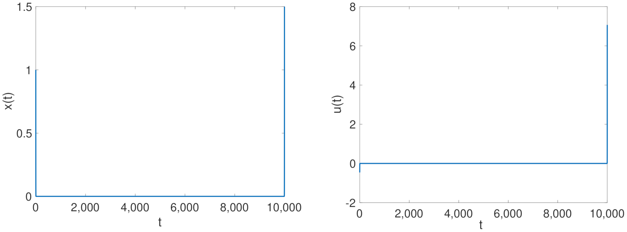
In Figure 1 we show the solution for $T=20$ and $T=40$. In

Table 1. Nonlinear Mass spring: final mesh (fM), total number of vectorized function evaluation (NVF) and mixed errors for $x,v,u$. The solution is computed starting from an initial mesh with 16 equidistant points.

	$\mathit{t}\mathit{o}\mathit{l}={10}^{-4}$
	$\mathit{T}=20$					$\mathit{T}=2\times {10}^4$
	fM	NVF	Error x	Error v	Error u	fM	NVF	Error x	Error v	Error u
bvp4c	71	35	$6.0\times {10}^{-6}$	$9.8\times {10}^{-6}$	$1.7\times {10}^{-5}$	*	*	*	*	*
bvp5c	294	1001	$9.0\times {10}^{-9}$	$2.0\times {10}^{-8}$	$4.7\times {10}^{-8}$	*	*	*	*	*
twpbvp_m	23	52	$2.5\times {10}^{-6}$	$4.4\times {10}^{-6}$	$4.8\times {10}^{-6}$	158	263	$3.8\times {10}^{-6}$	$2.4\times {10}^{-6}$	$3.0\times {10}^{-7}$
twpbvpc_m	38	52	$2.4\times {10}^{-6}$	$4.5\times {10}^{-6}$	$5.1\times {10}^{-6}$	201	246	$1.2\times {10}^{-6}$	$1.7\times {10}^{-6}$	$2.3\times {10}^{-6}$
twpbvp_l	27	54	$1.7\times {10}^{-6}$	$2.1\times {10}^{-6}$	$4.4\times {10}^{-6}$	97	200	$6.9\times {10}^{-6}$	$1.1\times {10}^{-5}$	$3.2\times {10}^{-5}$
twpbvpc_l	27	54	$1.7\times {10}^{-6}$	$2.1\times {10}^{-6}$	$4.4\times {10}^{-6}$	104	246	$5.7\times {10}^{-6}$	$6.2\times {10}^{-6}$	$2.8\times {10}^{-5}$
tom	116	14	$2.8\times {10}^{-6}$	$1.7\times {10}^{-6}$	$3.1\times {10}^{-6}$	426	30	$7.7\times {10}^{-6}$	$4.5\times {10}^{-6}$	$7.6\times {10}^{-6}$
tomc	136	16	$1.2\times {10}^{-6}$	$1.6\times {10}^{-6}$	$2.4\times {10}^{-6}$	526	41	$7.5\times {10}^{-7}$	$1.1\times {10}^{-6}$	$1.5\times {10}^{-6}$
	$\mathit{t}\mathit{o}\mathit{l}={\mathbf{10}}^{-\mathbf{6}}$
bvp4c	254	49	$2.4\times {10}^{-8}$	$6.6\times {10}^{-8}$	$1.5\times {10}^{-7}$	*	*	*	*	*
bvp5c	392	1221	$1.2\times {10}^{-10}$	$1.2\times {10}^{-10}$	$1.7\times {10}^{-10}$	*	*	*	*	*
twpbvp_m	42	50	$1.1\times {10}^{-8}$	$1.3\times {10}^{-8}$	$2.3\times {10}^{-8}$	254	271	$1.3\times {10}^{-7}$	$1.0\times {10}^{-7}$	$1.1\times {10}^{-7}$
twpbvpc_m	57	73	$3.2\times {10}^{-8}$	$4.4\times {10}^{-8}$	$5.0\times {10}^{-8}$	306	306	$8.1\times {10}^{-7}$	$7.1\times {10}^{-7}$	$6.3\times {10}^{-7}$
twpbvp_l	48	78	$2.0\times {10}^{-8}$	$1.9\times {10}^{-8}$	$2.3\times {10}^{-8}$	152	207	$1.7\times {10}^{-8}$	$2.2\times {10}^{-8}$	$2.5\times {10}^{-8}$
twpbvpc_l	58	78	$2.0\times {10}^{-8}$	$1.9\times {10}^{-8}$	$2.3\times {10}^{-8}$	136	253	$1.7\times {10}^{-8}$	$2.2\times {10}^{-8}$	$2.5\times {10}^{-8}$
tom	196	19	$1.6\times {10}^{-7}$	$2.2\times {10}^{-7}$	$2.8\times {10}^{-7}$	481	33	$4.5\times {10}^{-7}$	$4.1\times {10}^{-7}$	$5.1\times {10}^{-7}$
tomc	166	17	$7.2\times {10}^{-7}$	$6.8\times {10}^{-7}$	$7.4\times {10}^{-7}$	511	44	$2.1\times {10}^{-7}$	$2.7\times {10}^{-7}$	$3.1\times {10}^{-7}$

we present some results obtained increasing the value of T from 20 to $T=2\times {10}^6$. First, we choose an initial mesh of 16 equidistant points and try to run all the codes, except the codes acdc and acdcc, since for this formulation of the problem there is not a parameter to be used for continuation. If on one hand, for $T=20$ all the methods converge to the solution, and for $T=2\times {10}^4$ only the codes bvp4c and bvp5 fail, on the other hand for $T=2\times {10}^6$ no one goes to convergence except the codes tom and tomc (see

Table 2. Nonlinear Mass spring, $T=2\times {10}^6$: final mesh (fM), total number of vectorized function evaluation (NVF) and mixed errors for $x,v,u$, initial mesh with 16 equidistant points.

	fM	NVF	Error x	Error v	Error u	fVM	NVF	Error x	Error v	Error u
tom	6266	256	$6.4\times {10}^{-7}$	$8.9\times {10}^{-7}$	$1.1\times {10}^{-6}$	6266	256	$6.4\times {10}^{-7}$	$8.9\times {10}^{-7}$	$1.1\times {10}^{-6}$
tomc	1291	177	$6.6\times {10}^{-7}$	$7.5\times {10}^{-7}$	$1.4\times {10}^{-6}$	1236	180	$1.7\times {10}^{-7}$	$1.6\times {10}^{-7}$	$1.8\times {10}^{-7}$

). Essentially, there are some troubles with a singular Jacobian for bvp4c and bvp5c, or a drawback with the maximum number of mesh points allowed with the other codes. In the last case we could increase the maximum value of mesh points; however, we will try to differently overcome this matter and to debunk the idea that the indirect methods are not as competitive as direct ones.

First, we point out that the results presented in Table 2 clearly show that the mesh selection based on conditioning allows the solution of the problem using a reduced number of mesh points and vectorial function evaluations. To gain the convergence for the other codes, it can be sufficient, in some cases, to increase the number of points in the initial mesh. To this aim, in

Table 3. Nonlinear Mass spring, initial mesh (IM) with 501, 1001 and 2501 equidistant points and $T=2\times {10}^4$: final mesh (fM), total number of vectorized function evaluation (NVF) and mixed errors for $x,v,u$.

	IM	fM	NVF	Error x	Error v	Error u
bvp4c	2501	421	57	$9.5\times {10}^{-6}$	$1.1\times {10}^{-5}$	$1.0\times {10}^{-5}$
bvp5c	501	261	7200	$4.2\times {10}^{-6}$	$4.9\times {10}^{-6}$	$4.8\times {10}^{-6}$
bvp5c	1001	641	13,088	$4.1\times {10}^{-6}$	$4.7\times {10}^{-6}$	$4.6\times {10}^{-6}$
$\mathit{t}\mathit{o}\mathit{l}={\mathbf{10}}^{-\mathbf{6}}$
bvp4c	2501	471	71	$1.4\times {10}^{-7}$	$1.4\times {10}^{-7}$	$1.5\times {10}^{-7}$
bvp5c	501	333	7578	$3.9\times {10}^{-8}$	$5.7\times {10}^{-8}$	$6.1\times {10}^{-8}$
bvp5c	1001	512	13,880	$3.9\times {10}^{-8}$	$5.7\times {10}^{-8}$	$6.1\times {10}^{-8}$

we show the numerical results obtained for bvp5c using 501 or 1001 initial equidistant points and $T=2\times {10}^4$. This strategy is advantageous for bvp5c, not yet for bvp4c, that needs an initial mesh of 2501 mesh points to reach the convergence. However, we observe that bvp5c is not able to reach convergence if we use an initial mesh of 2501 mesh points. For the other classes of methods increasing the number of mesh points is not advantageous in terms of computational cost and time execution.

To improve the performance of all considered codes, the BVP (3) is reformulated using a variable transformation. Let $\tau =t/T$ with $\tau \in [0,1]$, we solve the following BVP

$$\begin{array}{cc}\hfill x^{\prime }& =Tv\hfill \\ \hfill v^{\prime }& =-T(x+x^3+\mu )\hfill \\ \hfill {\lambda }^{\prime }& =T\left(-x+\mu (1+3x^2)\right)\hfill \\ \hfill {\mu }^{\prime }& =-T\left(v+\lambda \right)\hfill \\ \hfill x\left(0\right)& =1,v\left(0\right)=0,x\left(1\right)=0.75,v\left(1\right)=0.\hfill \end{array}$$

(4)

Now, we set the perturbation parameter $ϵ=1/T$, so that we can run for parameters less than 1 the codes acdc and acdcc that use an automatic continuation strategy. For all the other codes, we can adopt a continuation strategy starting with an initial value of ${ϵ}_0$ that guarantees the convergence, in our case we use ${ϵ}_0=1/20$ and we change this value up to reach the required value. To this aim we consider the perturbation parameter changing in the interval $[{ϵ}_0,ϵ]$ among the values $0.5\times {10}^{-j},j=-2,\cdots ,-6$. This means that we discretize the interval with $N_{ϵ}=3$ and $N_{ϵ}=5$ respectively for $T=2\times {10}^4$ and $T=2\times {10}^6$. In

Table 4. Nonlinear Mass spring using the variable $\tau =t/T$, initial mesh with starting mesh with 11 equidistant points and continuation strategy on $ϵ=1/T$, final mesh (fM), total number of vectorized function evaluation (NVF) and mixed errors for $x,v,u$.

	$\mathit{t}\mathit{o}\mathit{l}={10}^{-4}$
	$\mathit{T}=20$					$\mathit{T}=2\times {10}^4$					$\mathit{T}=2\times {10}^6$
	fM	NVF	Error x	Error v	Error u	fM	NVF	Error x	Error v	Error u	fM	NVF	Error x	Error v	Error u
bvp4c	78	45	$6.3\times {10}^{-6}$	$9.6\times {10}^{-6}$	$2.8\times {10}^{-5}$	199	178	$4.3\times {10}^{-4}$	$4.5\times {10}^{-4}$	$5.9\times {10}^{-4}$	2093	334	$2.5\times {10}^{-3}$	$3.5\times {10}^{-3}$	$3.5\times {10}^{-3}$
bvp5c	38	220	$1.6\times {10}^{-6}$	$1.1\times {10}^{-6}$	$9.5\times {10}^{-7}$	148	1658	$3.3\times {10}^{-6}$	$7.1\times {10}^{-6}$	$8.4\times {10}^{-6}$	1784	11,712	$3.0\times {10}^{-6}$	$4.5\times {10}^{-6}$	$4.8\times {10}^{-6}$
twpbvp_m	24	56	$1.4\times {10}^{-6}$	$9.2\times {10}^{-7}$	$1.3\times {10}^{-6}$	137	233	$6.8\times {10}^{-5}$	$8.2\times {10}^{-5}$	$9.2\times {10}^{-5}$	163	358	$2.6\times {10}^{-6}$	$2.9\times {10}^{-6}$	$2.9\times {10}^{-6}$
twpbvpc_m	39	81	$3.2\times {10}^{-6}$	$1.9\times {10}^{-6}$	$2.3\times {10}^{-6}$	421	221	$3.5\times {10}^{-6}$	$2.6\times {10}^{-6}$	$2.0\times {10}^{-6}$	141	335	$2.5\times {10}^{-5}$	$4.8\times {10}^{-5}$	$6.8\times {10}^{-5}$
twpbvp_l	28	51	$6.3\times {10}^{-6}$	$9.6\times {10}^{-6}$	$2.8\times {10}^{-5}$	76	346	$1.1\times {10}^{-5}$	$1.4\times {10}^{-5}$	$1.9\times {10}^{-5}$	83	557	$1.1\times {10}^{-5}$	$1.4\times {10}^{-5}$	$1.9\times {10}^{-5}$
twpbvpc_l	28	51	$6.3\times {10}^{-6}$	$9.6\times {10}^{-6}$	$2.8\times {10}^{-5}$	102	237	$6.0\times {10}^{-6}$	$9.4\times {10}^{-6}$	$1.1\times {10}^{-5}$	139	343	$6.0\times {10}^{-6}$	$9.4\times {10}^{-6}$	$1.1\times {10}^{-5}$
tom	156	16	$7.3\times {10}^{-7}$	$1.2\times {10}^{-6}$	$1.5\times {10}^{-6}$	481	49	$1.1\times {10}^{-5}$	$6.7\times {10}^{-6}$	$1.1\times {10}^{-5}$	711	73	$7.0\times {10}^{-7}$	$6.9\times {10}^{-7}$	$8.1\times {10}^{-7}$
tomc	141	16	$1.6\times {10}^{-6}$	$1.1\times {10}^{-6}$	$2.6\times {10}^{-6}$	681	31	$1.6\times {10}^{-6}$	$2.1\times {10}^{-6}$	$2.4\times {10}^{-6}$	1356	49	$9.0\times {10}^{-8}$	$1.7\times {10}^{-7}$	$2.4\times {10}^{-7}$
acdc	25	155	$2.8\times {10}^{-5}$	$2.7\times {10}^{-5}$	$3.0\times {10}^{-5}$	66	485	$2.6\times {10}^{-6}$	$4.0\times {10}^{-6}$	$6.2\times {10}^{-6}$	110	749	$2.9\times {10}^{-6}$	$1.6\times {10}^{-6}$	$3.3\times {10}^{-6}$
acdcc	25	155	$2.8\times {10}^{-5}$	$2.7\times {10}^{-5}$	$3.0\times {10}^{-5}$	106	375	$2.3\times {10}^{-5}$	$1.4\times {10}^{-5}$	$1.5\times {10}^{-5}$	176	501	$2.3\times {10}^{-5}$	$3.0\times {10}^{-5}$	$3.7\times {10}^{-5}$
	$\mathit{t}\mathit{o}\mathit{l}={\mathbf{10}}^{-\mathbf{6}}$
bvp4c	296	57	$2.6\times {10}^{-8}$	$2.5\times {10}^{-8}$	$2.8\times {10}^{-8}$	319	160	$1.6\times {10}^{-6}$	$2.0\times {10}^{-6}$	$2.6\times {10}^{-6}$	374	280	$1.5\times {10}^{-5}$	$1.6\times {10}^{-5}$	$1.7\times {10}^{-5}$
bvp5c	87	464	$1.2\times {10}^{-8}$	$9.3\times {10}^{-9}$	$4.9\times {10}^{-9}$	203	3535	$1.4\times {10}^{-8}$	$1.9\times {10}^{-8}$	$2.7\times {10}^{-8}$	1305	19,524	$2.5\times {10}^{-8}$	$4.0\times {10}^{-8}$	$4.4\times {10}^{-8}$
twpbvp_m	39	83	$8.2\times {10}^{-8}$	$8.7\times {10}^{-8}$	$9.5\times {10}^{-8}$	178	341	$7.0\times {10}^{-8}$	$8.8\times {10}^{-8}$	$9.2\times {10}^{-8}$	497	459	$5.4\times {10}^{-9}$	$7.1\times {10}^{-9}$	$8.3\times {10}^{-9}$
twpbvpc_m	50	83	$8.2\times {10}^{-8}$	$8.7\times {10}^{-8}$	$9.5\times {10}^{-8}$	190	255	$7.9\times {10}^{-8}$	$5.5\times {10}^{-8}$	$6.4\times {10}^{-8}$	423	375	$8.1\times {10}^{-9}$	$8.1\times {10}^{-9}$	$8.9\times {10}^{-9}$
twpbvp_l	50	90	$9.8\times {10}^{-9}$	$1.1\times {10}^{-8}$	$1.2\times {10}^{-8}$	114	284	$1.9\times {10}^{-8}$	$2.5\times {10}^{-8}$	$1.0\times {10}^{-7}$	103	446	$1.0\times {10}^{-8}$	$1.1\times {10}^{-8}$	$1.7\times {10}^{-8}$
twpbvpc_l	61	90	$9.8\times {10}^{-9}$	$1.1\times {10}^{-8}$	$1.2\times {10}^{-8}$	120	246	$2.4\times {10}^{-8}$	$2.2\times {10}^{-8}$	$3.3\times {10}^{-8}$	127	350	$2.4\times {10}^{-8}$	$2.2\times {10}^{-8}$	$3.3\times {10}^{-8}$
tom	161	17	$8.0\times {10}^{-7}$	$1.3\times {10}^{-6}$	$1.6\times {10}^{-6}$	426	62	$5.8\times {10}^{-7}$	$7.6\times {10}^{-7}$	$9.4\times {10}^{-7}$	751	95	$2.1\times {10}^{-7}$	$2.6\times {10}^{-7}$	$2.9\times {10}^{-7}$
tomc	186	19	$2.1\times {10}^{-7}$	$4.1\times {10}^{-7}$	$4.5\times {10}^{-7}$	831	36	$2.4\times {10}^{-7}$	$2.0\times {10}^{-7}$	$2.5\times {10}^{-7}$	826	56	$2.2\times {10}^{-7}$	$2.3\times {10}^{-7}$	$2.6\times {10}^{-7}$
acdc	50	158	$1.4\times {10}^{-8}$	$1.8\times {10}^{-8}$	$2.1\times {10}^{-8}$	95	382	$1.0\times {10}^{-8}$	$1.8\times {10}^{-8}$	$2.0\times {10}^{-8}$	89	581	$2.7\times {10}^{-8}$	$3.8\times {10}^{-8}$	$4.4\times {10}^{-8}$
acdcc	50	158	$1.4\times {10}^{-8}$	$1.8\times {10}^{-8}$	$2.1\times {10}^{-8}$	183	371	$1.8\times {10}^{-7}$	$2.0\times {10}^{-7}$	$2.1\times {10}^{-7}$	184	513	$1.8\times {10}^{-7}$	$2.0\times {10}^{-7}$	$2.1\times {10}^{-7}$

we show the results obtained applying this successful continuation strategy. All the methods converge for all the values of T using a low computational cost. In this case, the codes based on automatic continuation strategy are very efficient, using acdc/acdcc the users do not need to decide how to change the continuation parameters, even if in some cases the automatic continuation could fail to reach the final desired value.

More information about this problem could be obtained by analyzing the conditioning parameters given in output by the codes twpbvpc_m and tomc, reported in  

Table 5. Nonlinear Mass spring: conditioning parameters computed using $tol={10}^{-6}$ and initial mesh with 11 equidistant points.

	$\mathit{\sigma }$	$\mathit{\kappa }$	${\mathit{\kappa }}_1$	${\mathit{\kappa }}_2$	${\mathit{\gamma }}_1$
$T=20$
twpbvpc_m	$1.90\times {10}^1$	$1.33\times {10}^1$	$4.72\times {10}^0$	$8.57\times {10}^0$	$2.16\times {10}^{-1}$
tomc	$2.04\times {10}^1$	$1.33\times {10}^1$	$4.79\times {10}^0$	$8.61\times {10}^0$	$5.28\times {10}^{-1}$
$T=2\times {10}^4$
twpbvpc_m	$1.97\times {10}^4$	$1.34\times {10}^1$	$4.73\times {10}^0$	$8.65\times {10}^0$	$5.09\times {10}^{-4}$
tomc	$2.08\times {10}^4$	$1.66\times {10}^1$	$5.42\times {10}^0$	$1.12\times {10}^1$	$2.11\times {10}^{-4}$
$T=2\times {10}^6$
twpbvpc_m	$1.90\times {10}^6$	$1.34\times {10}^1$	$4.75\times {10}^0$	$8.61\times {10}^0$	$5.28\times {10}^{-6}$
tomc	$2.03\times {10}^6$	$1.66\times {10}^1$	$5.45\times {10}^0$	$1.11\times {10}^1$	$2.17\times {10}^{-6}$

. As we can see the stiffness parameter $\sigma$ grows with the width of the interval, and depends on this last, moreover ${\kappa }_2>{\kappa }_1$ shows that the problem could be ill posed, and ${\gamma }_1$ tending to zeros shows the presence of different time scales. The transformation of time interval in $[0,1]$ does not change the stiffness of the problem, but the problem is well posed (see 

Table 6. Nonlinear Mass spring using the variable $\tau =t/T$: conditioning parameters computed using $tol={10}^{-6}$ and initial mesh with 11 equidistant points.

	$\mathit{\sigma }$	$\mathit{\kappa }$	${\mathit{\kappa }}_1$	${\mathit{\kappa }}_2$	${\mathit{\gamma }}_1$
$T=20$
twpbvpc_m	$1.90\times {10}^1$	$5.15\times {10}^0$	$4.72\times {10}^0$	$4.31\times {10}^{-1}$	$5.28\times {10}^{-1}$
tomc	$2.06\times {10}^1$	$5.18\times {10}^0$	$4.75\times {10}^0$	$4.30\times {10}^{-1}$	$2.12\times {10}^{-1}$
$T=2\times {10}^4$
twpbvpc_m	$1.90\times {10}^4$	$4.73\times {10}^0$	$4.73\times {10}^0$	$4.30\times {10}^{-4}$	$5.26\times {10}^{-4}$
tomc	$2.08\times {10}^4$	$4.75\times {10}^0$	$4.75\times {10}^0$	$4.31\times {10}^{-4}$	$2.10\times {10}^{-4}$
$T=2\times {10}^6$
twpbvpc_m	$1.90\times {10}^6$	$4.75\times {10}^0$	$4.75\times {10}^0$	$4.31\times {10}^{-6}$	$5.28\times {10}^{-6}$
tomc	$2.09\times {10}^6$	$4.75\times {10}^0$	$4.75\times {10}^0$	$4.31\times {10}^{-6}$	$2.09\times {10}^{-6}$

).

4.2. Completely Hypersensitive Control Problem

This example is a hypersensitive optimal control problem implemented in ICLOCS2, defined as a problem “extremely difficult” to solve using an indirect method [42,44] and given by

$$\left\{\begin{array}{c}{\displaystyle \underset{x,u}{min}{\int }_0^T(x^2+u^2)dt}\hfill \\ x^{\prime }=-x^3+u\hfill \\ x\left(0\right)=1,x\left(T\right)=1.5.\hfill \end{array}\right.$$

(5)

Considered the Hamiltonian $H(x,\lambda ,u)=x^2+u^2+\lambda (-x^3+u)$, the first-order necessary conditions for optimality leads to the following boundary value problem (BVP)

$$\begin{array}{cc}\hfill x^{\prime }& =-x^3-\frac{\lambda }{2}\hfill \\ \hfill {\lambda }^{\prime }& =-2x+3\lambda x^2\hfill \\ \hfill x\left(0\right)& =1,x\left(T\right)=1.5,\hfill \end{array}$$

(6)

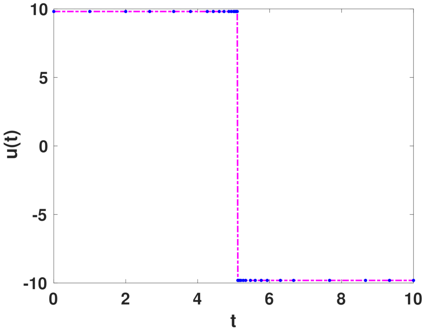
where the optimal control is $u^{*}=-\frac{\lambda }{2}$. We choose $T={10}^4,T={10}^6$ and an initial mesh of 11 equidistant points, the solution is plotted in Figure 2. Numerical results shown in  

Table 7. Hypersensitive problem solved with an initial mesh with 11 equidistant points: final mesh (fM), total number of vectorized function evaluation (NVF) and mixed errors for $x,v,u$.

	fM	NVF	Error x	Error v	Error u	fM	NVF	Error x	Error v	Error u
twpbvp_m	117	239	$1.5\times {10}^{-6}$	$3.1\times {10}^{-6}$	$1.5\times {10}^{-6}$	1821	394	$1.9\times {10}^{-5}$	$3.8\times {10}^{-5}$	$1.9\times {10}^{-5}$
twpbvpc_m	140	237	$1.7\times {10}^{-6}$	$3.4\times {10}^{-6}$	$1.7\times {10}^{-6}$	650	456	$3.3\times {10}^{-5}$	$6.7\times {10}^{-5}$	$5.0\times {10}^{-5}$
twpbvp_l	105	224	$7.0\times {10}^{-6}$	$2.7\times {10}^{-5}$	$1.7\times {10}^{-5}$	*	*	*	*	*
twpbvpc_l	91	286	$6.6\times {10}^{-9}$	$1.3\times {10}^{-8}$	$6.6\times {10}^{-9}$	1176	425	$8.2\times {10}^{-9}$	$3.0\times {10}^{-8}$	$1.9\times {10}^{-8}$
tom	691	33	$2.8\times {10}^{-9}$	$5.5\times {10}^{-9}$	$2.8\times {10}^{-9}$	636	169	$2.5\times {10}^{-6}$	$2.3\times {10}^{-5}$	$2.1\times {10}^{-5}$
tomc	681	46	$5.7\times {10}^{-7}$	$1.1\times {10}^{-6}$	$5.7\times {10}^{-7}$	1941	134	$4.0\times {10}^{-9}$	$8.0\times {10}^{-9}$	$4.0\times {10}^{-9}$
	$\mathit{t}\mathit{o}\mathit{l}={\mathbf{10}}^{-\mathbf{6}}$
twpbvp_m	357	245	$9.8\times {10}^{-9}$	$2.0\times {10}^{-8}$	$1.3\times {10}^{-8}$	1859	392	$2.6\times {10}^{-8}$	$5.3\times {10}^{-8}$	$2.6\times {10}^{-8}$
twpbvpc_m	265	239	$3.2\times {10}^{-7}$	$6.4\times {10}^{-7}$	$3.2\times {10}^{-7}$	536	475	$4.4\times {10}^{-8}$	$8.8\times {10}^{-8}$	$4.4\times {10}^{-8}$
twpbvp_l	94	248	$5.3\times {10}^{-8}$	$1.1\times {10}^{-7}$	$5.3\times {10}^{-8}$	*	*	*	*	*
twpbvpc_l	91	286	$6.6\times {10}^{-9}$	$1.3\times {10}^{-8}$	$6.6\times {10}^{-9}$	1176	425	$8.2\times {10}^{-9}$	$3.0\times {10}^{-8}$	$1.9\times {10}^{-8}$
tom	691	33	$2.8\times {10}^{-9}$	$5.5\times {10}^{-9}$	$2.8\times {10}^{-9}$	691	172	$8.8\times {10}^{-8}$	$2.5\times {10}^{-7}$	$2.3\times {10}^{-7}$
tomc	681	46	$5.7\times {10}^{-7}$	$1.1\times {10}^{-6}$	$5.7\times {10}^{-7}$	1941	134	$4.0\times {10}^{-9}$	$8.0\times {10}^{-9}$	$4.0\times {10}^{-9}$

point out good performance of all the codes except bvp4c and bvp5c, which are not suitable for stiff problems, indeed we underline as they converge to the solution respectively up to $T=38$ and $T=29$.

In  

Table 8. Hypersensitive problem: conditioning parameters computed using $tol={10}^{-6}$ and initial mesh with 11 equidistant points.

	$\mathit{\sigma }$	$\mathit{\kappa }$	${\mathit{\kappa }}_1$	${\mathit{\kappa }}_2$	${\mathit{\gamma }}_1$
$T=10$
twpbvpc_m	$5.94\times {10}^1$	$3.09\times {10}^1$	$2.67\times {10}^1$	$4.23\times {10}^0$	$5.51\times {10}^{-1}$
twpbvpc_l	$5.95\times {10}^1$	$3.09\times {10}^1$	$2.67\times {10}^1$	$4.23\times {10}^0$	$5.49\times {10}^{-1}$
tomc	$6.83\times {10}^1$	$3.09\times {10}^1$	$2.67\times {10}^1$	$4.23\times {10}^0$	$3.90\times {10}^{-1}$
$T={10}^4$
twpbvpc_m	$6.34\times {10}^4$	$3.09\times {10}^1$	$2.66\times {10}^1$	$4.23\times {10}^0$	$5.24\times {10}^{-4}$
twpbvpc_l	$5.80\times {10}^4$	$3.09\times {10}^1$	$2.67\times {10}^1$	$4.23\times {10}^0$	$5.61\times {10}^{-4}$
tomc	$6.74\times {10}^4$	$3.09\times {10}^1$	$2.66\times {10}^1$	$4.23\times {10}^0$	$3.96\times {10}^{-4}$
$T={10}^6$
twpbvpc_m	$6.44\times {10}^6$	$3.09\times {10}^1$	$2.66\times {10}^1$	$4.23\times {10}^0$	$5.11\times {10}^{-6}$
twpbvpc_l	$5.97\times {10}^6$	$3.09\times {10}^1$	$2.67\times {10}^1$	$4.23\times {10}^0$	$5.54\times {10}^{-6}$
tomc	$6.92\times {10}^6$	$4.70\times {10}^1$	$9.15\times {10}^0$	$3.78\times {10}^1$	$3.85\times {10}^{-6}$

the approximations of the conditioning constants show the dependence of the stiffness on the width of the interval. Moreover, the numerical results underline the necessity of adopting a good mesh selection strategy for computing the solution.

For the purpose of improving the performance and overcoming some drawbacks, we propose, as already done for the test problem in Section 4.1, to use the transformation of the variable $\tau =t/T$, such that the BVP (6) can be reformulated for $\tau \in [0,1]$ as

$$\begin{array}{cc}\hfill x^{\prime }& =T\left(-x^3-\frac{\lambda }{2}\right)\hfill \\ \hfill {\lambda }^{\prime }& =T\left(-2x+3\lambda x^2\right)\hfill \\ \hfill x\left(0\right)& =1,x\left(1\right)=1.5.\hfill \end{array}$$

(7)

The advantage of this formulation is that considering $ϵ=1/T$ as a perturbation parameter, we can apply the continuation strategy on that parameter. In

Table 9. Hypersensitive problem using the variable $\tau =t/T$, initial mesh with 11 equidistant points and continuation strategy on T: final mesh (fM), total number of vectorized function evaluation (NVF) and mixed errors for x,v,u.

	$\mathit{T}={10}^4$
	$\mathit{t}\mathit{o}\mathit{l}={10}^{-4}$					$\mathit{t}\mathit{o}\mathit{l}={10}^{-6}$
	fM	NVF	Error x	Error v	Error u	fM	NVF	Error x	Error v	Error u
bvp4c	107	198	$1.1\times {10}^{-4}$	$4.5\times {10}^{-4}$	$3.8\times {10}^{-4}$	242	170	$1.1\times {10}^{-6}$	$4.6\times {10}^{-6}$	$3.6\times {10}^{-6}$
bvp5c	70	1277	$8.5\times {10}^{-7}$	$1.7\times {10}^{-6}$	$8.5\times {10}^{-7}$	132	2874	$4.9\times {10}^{-9}$	$9.8\times {10}^{-9}$	$4.9\times {10}^{-9}$
twpbvp_m	59	266	$2.2\times {10}^{-5}$	$4.4\times {10}^{-5}$	$2.2\times {10}^{-5}$	124	311	$4.9\times {10}^{-6}$	$8.1\times {10}^{-6}$	$4.9\times {10}^{-6}$
twpbvpc_m	101	210	$9.1\times {10}^{-5}$	$1.8\times {10}^{-4}$	$9.1\times {10}^{-5}$	190	226	$9.5\times {10}^{-8}$	$1.9\times {10}^{-7}$	$9.5\times {10}^{-8}$
twpbvp_l	45	389	$3.5\times {10}^{-6}$	$1.9\times {10}^{-5}$	$1.8\times {10}^{-5}$	63	306	$4.9\times {10}^{-8}$	$1.9\times {10}^{-7}$	$1.8\times {10}^{-7}$
twpbvpc_l	76	229	$1.3\times {10}^{-5}$	$2.6\times {10}^{-5}$	$1.3\times {10}^{-5}$	79	234	$4.7\times {10}^{-8}$	$9.4\times {10}^{-8}$	$4.7\times {10}^{-8}$
tom	571	56	$7.9\times {10}^{-7}$	$1.8\times {10}^{-7}$	$1.2\times {10}^{-7}$	746	59	$1.1\times {10}^{-8}$	$2.6\times {10}^{-8}$	$2.1\times {10}^{-8}$
tomc	951	46	$4.9\times {10}^{-9}$	$7.2\times {10}^{-9}$	$5.8\times {10}^{-9}$	1231	52	$1.2\times {10}^{-8}$	$3.7\times {10}^{-9}$	$2.3\times {10}^{-9}$
acdc	56	491	$4.0\times {10}^{-6}$	$1.5\times {10}^{-5}$	$1.4\times {10}^{-5}$	60	425	$5.7\times {10}^{-8}$	$1.9\times {10}^{-7}$	$1.7\times {10}^{-7}$
acdcc	130	672	$2.1\times {10}^{-5}$	$5.6\times {10}^{-5}$	$3.6\times {10}^{-5}$	144	478	$5.2\times {10}^{-8}$	$1.8\times {10}^{-7}$	$1.2\times {10}^{-7}$

we report the results using as starting value ${ϵ}_0=1/10$ and changing the continuation parameters in the interval $[{ϵ}_0,ϵ]$ among the value of the set ${10}^{-2},{10}^{-3},{10}^{-4}$. We remember that acdc and acdcc, using an automatic continuation strategy, needs only to insert the desired value of $ϵ$ and uses as ${ϵ}_0$ the default value $0.5$. The numerical tests and the conditioning parameters in Table 8 and

Table 10. Hypersensitive problem using the variable $\tau =t/T$: conditioning parameters computed using $tol={10}^{-6}$ and initial mesh with 11 equidistant points.

	$\mathit{\sigma }$	$\mathit{\kappa }$	${\mathit{\kappa }}_1$	${\mathit{\kappa }}_2$	${\mathit{\gamma }}_1$
$T=10$
twpbvpc_m	$5.94\times {10}^1$	$2.71\times {10}^1$	$2.67\times {10}^1$	$4.23\times {10}^{-1}$	$5.51\times {10}^{-1}$
twpbvpc_l	$5.95\times {10}^1$	$2.71\times {10}^1$	$2.67\times {10}^1$	$4.23\times {10}^{-1}$	$5.49\times {10}^{-1}$
tomc	$6.86\times {10}^1$	$2.71\times {10}^1$	$2.66\times {10}^1$	$4.23\times {10}^{-1}$	$3.88\times {10}^{-1}$
$T={10}^4$
twpbvpc_m	$6.34\times {10}^4$	$2.66\times {10}^1$	$2.66\times {10}^1$	$4.23\times {10}^{-4}$	$5.24\times {10}^{-4}$
twpbvpc_l	$5.80\times {10}^4$	$2.67\times {10}^1$	$2.67\times {10}^1$	$4.23\times {10}^{-4}$	$5.61\times {10}^{-4}$
tomc	$6.74\times {10}^4$	$2.66\times {10}^1$	$2.66\times {10}^1$	$4.23\times {10}^{-4}$	$3.95\times {10}^{-4}$
$T={10}^6$
twpbvpc_m	$6.52\times {10}^6$	$2.66\times {10}^1$	$2.66\times {10}^1$	$4.23\times {10}^{-6}$	$5.06\times {10}^{-6}$
twpbvpc_l	$5.72\times {10}^6$	$2.67\times {10}^1$	$2.67\times {10}^1$	$4.23\times {10}^{-6}$	$5.72\times {10}^{-6}$
tomc	$6.87\times {10}^6$	$2.66\times {10}^1$	$2.66\times {10}^1$	$4.23\times {10}^{-6}$	$3.88\times {10}^{-6}$

clearly show that for this class of problems, if we cannot use a continuation of parameters, the codes able to give a solution are the ones suited for stiff problems that work still better if also the mesh selection is appropriate for this class of problems.

5. Bang-Bang Optimal Control Problem

The bang-bang optimal control problem [45] is among the more challenging ones. It arises from a model in which a point unit mass m subjects to a limited force in one-dimensional space, i.e., $m{x}^{″}\left(t\right)=u\left(t\right)$ and $u\left(t\right)\le 1$. The main feature of optimal control problem of moving the mass from $x=0$ to the maximum distance x in one second can be formulated as follows

$$\begin{array}{cc}\hfill min-x\left(1\right)& ={\int }_0^1(-v)dt,\hfill \\ \hfill x^{\prime }& =v,\hfill \\ \hfill v^{\prime }& =u,t\in [0,1],\hfill \\ \hfill x\left(0\right)& =v\left(0\right)=v\left(1\right)=0,\hfill \\ \hfill \left|u\right|& \le 1,\hfill \end{array}$$

(8)

The associated Hamiltonian function is defined as

$$H(x,v,\lambda ,\mu ,u)=-v+\lambda v+\mu u$$

and the optimal control is given by

$$u^{*}=\underset{\left|u\right|\le 1}{arg\; min}H(x,v,\lambda ,\mu ,u)=-sign\left(\mu \right).$$

Now, by applying the indirect method the solution of the optimal control Problem (8) is equivalent to solve the following BVP problem

$$\begin{array}{cc}\hfill x^{\prime }& =v,\hfill \\ \hfill v^{\prime }& =u,\hfill \\ \hfill {\lambda }^{\prime }& =0,\hfill \\ \hfill {\mu }^{\prime }& =1-\lambda ,\hfill \\ \hfill x\left(0\right)& =v\left(0\right)=v\left(1\right)=\lambda \left(1\right)=0.\hfill \end{array}$$

(9)

We observe that the optimal control is defined as

$$u\left(t\right)=-sign\left(\mu \right)=\left\{\begin{array}{cc}1\hfill & \mu <0,\hfill \\ -1\hfill & \mu >0,\hfill \\ \mathrm{any} \mathrm{value} \mathrm{in}[-1,1]\hfill & \mu =0,\hfill \end{array}\right.$$

and the exact solution is given by

$$\begin{array}{cc}x\left(t\right)=\left\{\begin{array}{cc}{\displaystyle \frac{t^2}{2}}\hfill & t<1/2\hfill \\ {\displaystyle t-\frac{t^2}{2}-\frac{1}{4}}\hfill & t>1/2\hfill \end{array}\right.,\hfill & v\left(t\right)=\left\{\begin{array}{cc}t\hfill & t<1/2\hfill \\ 1-t\hfill & t>1/2\hfill \end{array}\right.,\hfill \\ u\left(t\right)=\left\{\begin{array}{cc}1\hfill & t<1/2,\hfill \\ -1\hfill & t>1/2,\hfill \end{array}\right.,\hfill & {\displaystyle \lambda \left(t\right)=0,\mu \left(t\right)=t-\frac{1}{2}.}\hfill \end{array}$$

The discontinuity of the switching function is overcome by a smoothing technique that can be executed by different strategies. We choose two of them in particular. The first strategy, given a small parameter $ϵ$, consists of using the approximation

$$sign\left(\mu \right)\approx \frac{2}{\pi }arctan\left(\frac{\mu \pi }{2ϵ}\right).$$

The exact bang-bang solution is better approximated when $ϵ$ becomes smaller; however, this for value around smaller than ${10}^{-4}$ can give ill-conditioning problems.

Table 11. Bang-Bang optimal control Problem (9): final mesh (fM), total number of vectorized function evaluation (NVF) and mixed errors for x, v, u.

	$\mathit{t}\mathit{o}\mathit{l}={10}^{-4}$
	$\mathit{ϵ}={10}^{-3}$					$\mathit{ϵ}={10}^{-6}$
	fM	NVF	Error x	Error v	Error u	fM	NVF	Error x	Error v	Error u
bvp4c	25	51	$3.2\times {10}^{-4}$	$1.8\times {10}^{-3}$	0	27	97	$3.2\times {10}^{-7}$	$4.0\times {10}^{-6}$	0
twpbvp_m	16	11	$3.0\times {10}^{-4}$	$7.5\times {10}^{-4}$	0	16	11	$2.1\times {10}^{-5}$	$7.5\times {10}^{-7}$	0
twpbvp_l	16	13	$2.5\times {10}^{-4}$	$7.5\times {10}^{-4}$	0	16	13	$7.6\times {10}^{-5}$	$7.5\times {10}^{-7}$	0
tom	111	10	$3.2\times {10}^{-4}$	$1.0\times {10}^{-3}$	0	31	16	$1.8\times {10}^{-4}$	$8.8\times {10}^{-4}$	0
tomc	121	10	$3.2\times {10}^{-4}$	$1.0\times {10}^{-3}$	0	31	28	$1.8\times {10}^{-4}$	$8.8\times {10}^{-4}$	0
acdc	9	157	$3.2\times {10}^{-4}$	$8.7\times {10}^{-4}$	0	9	221	$3.2\times {10}^{-7}$	$1.5\times {10}^{-6}$	0
	$\mathit{t}\mathit{o}\mathit{l}={\mathbf{10}}^{-\mathbf{6}}$
bvp4c	79	57	$3.2\times {10}^{-4}$	$2.0\times {10}^{-3}$	0	47	93	$3.2\times {10}^{-7}$	$4.0\times {10}^{-6}$	0
twpbvp_m	10	32	$3.3\times {10}^{-4}$	$1.0\times {10}^{-3}$	0	10	32	$5.1\times {10}^{-6}$	$1.0\times {10}^{-6}$	0
twpbvp_l	17	66	$3.2\times {10}^{-4}$	$1.3\times {10}^{-3}$	0	15	130	$3.2\times {10}^{-7}$	$2.1\times {10}^{-6}$	0
tom	231	19	$3.2\times {10}^{-4}$	$1.1\times {10}^{-3}$	0	281	32	$3.3\times {10}^{-7}$	$1.1\times {10}^{-6}$	0
tomc	201	19	$3.2\times {10}^{-4}$	$1.1\times {10}^{-3}$	0	231	40	$3.3\times {10}^{-7}$	$1.1\times {10}^{-6}$	0
acdc	20	170	$3.2\times {10}^{-4}$	$1.3\times {10}^{-3}$	0	17	242	$3.2\times {10}^{-7}$	$2.2\times {10}^{-6}$	0

contains all the results obtained using the Matlab codes, the solution is plotted in Figure 3. Only bvp5c fails, and for getting the solution is necessary to use the continuation strategy. To this regard we consider as initial perturbation parameter ${ϵ}_0=1$ and then we change it choosing $N_{ϵ}=10$ logarithmically equispaced points between 1 and the value required $ϵ$. When $tol={10}^{-4}$bvp5c converges using 19 points for both $ϵ$ equal to ${10}^{-3}$ and ${10}^{-6}$, instead when $tol={10}^{-4}$bvp5c gets the solution with 36 and 28 points respectively for $ϵ={10}^{-3}$ and $ϵ={10}^{-6}$.

For the second smoothing technique we can add a barrier or a penalty function. In this regard, we consider a piecewise quadratic penalty function defined as in [45]

$$P(u;ϵ,\sigma )=\frac{ϵ}{2}{u}^2+\frac{1}{{\sigma }^2}\left\{\begin{array}{cc}{\left(\right|u|-1+\sigma )}^2\hfill & \hfill \left|u\right|>1-\sigma ,\\ 0\hfill & \hfill \mathrm{otherwise}\end{array}\right.$$

where the parameter $\sigma$ gives the distance from the border where the penalty changes fast.

Consequently, the Problem (8) is reformulated without inequality constraint as follows

$$\begin{array}{cc}\hfill min{\int }_0^1& P(u;ϵ,\sigma )-vdt,\hfill \\ \hfill x^{\prime }& =v,\hfill \\ \hfill v^{\prime }& =u,t\in [0,1],\hfill \\ \hfill x\left(0\right)& =v\left(0\right)=v\left(1\right)=0.\hfill \end{array}$$

(10)

The optimal control u, obtained as a solution of the equation

$$P_u(u;ϵ,\sigma )+\mu =0,$$

is equal to

$$u=\left\{\begin{array}{cc}{\displaystyle \frac{2-2\sigma -{\sigma }^2\mu }{ϵ{\sigma }^2+2}}\hfill & u\ge 1-\sigma \hfill \\ {\displaystyle \frac{-2+2\sigma -{\sigma }^2\mu }{ϵ{\sigma }^2+2}}\hfill & u<\sigma -1\hfill \\ 0\hfill & \mathrm{otherwise}.\hfill \end{array}\right.$$

In

Table 12. Bang-Bang optimal control problem-solving (8) using a piecewise quadratic penalty function with $\sigma ={10}^{-4}$: final mesh (fM), total number of vectorized function evaluation (NVF) and mixed errors for x, v, u.

	$\mathit{t}\mathit{o}\mathit{l}={10}^{-4}$
	$\mathit{ϵ}={10}^{-3}$					$\mathit{ϵ}={10}^{-6}$
	fM	NVF	Error x	Error v	Error u	fM	NVF	Error x	Error v	Error u
twpbvp_m	16	11	$9.8\times {10}^{-6}$	$3.2\times {10}^{-5}$	$5.0\times {10}^{-5}$	16	11	$9.8\times {10}^{-6}$	$3.2\times {10}^{-5}$	$5.0\times {10}^{-5}$
twpbvp_l	16	13	$6.4\times {10}^{-5}$	$3.2\times {10}^{-5}$	$5.0\times {10}^{-5}$	16	13	$6.4\times {10}^{-5}$	$3.2\times {10}^{-5}$	$5.0\times {10}^{-5}$
tom	111	10	$2.2\times {10}^{-5}$	$6.3\times {10}^{-5}$	$5.0\times {10}^{-5}$	31	27	$1.9\times {10}^{-4}$	$8.5\times {10}^{-4}$	$5.0\times {10}^{-5}$
tomc	126	9	$2.1\times {10}^{-5}$	$6.6\times {10}^{-5}$	$5.0\times {10}^{-5}$	31	20	$1.9\times {10}^{-4}$	$8.5\times {10}^{-4}$	$5.0\times {10}^{-5}$
	$\mathit{t}\mathit{o}\mathit{l}={\mathbf{10}}^{-\mathbf{6}}$
twpbvp_m	8	32	$2.4\times {10}^{-5}$	$3.3\times {10}^{-5}$	$5.0\times {10}^{-5}$	8	32	$2.4\times {10}^{-5}$	$3.3\times {10}^{-5}$	$5.0\times {10}^{-5}$
twpbvp_l	9	93	$2.0\times {10}^{-5}$	$3.3\times {10}^{-5}$	$5.0\times {10}^{-5}$	8	130	$2.0\times {10}^{-5}$	$3.7\times {10}^{-5}$	$5.0\times {10}^{-5}$
tom	231	19	$2.0\times {10}^{-5}$	$3.4\times {10}^{-5}$	$5.0\times {10}^{-5}$	381	51	$2.0\times {10}^{-5}$	$3.3\times {10}^{-5}$	$5.0\times {10}^{-5}$
tomc	261	20	$2.0\times {10}^{-5}$	$3.3\times {10}^{-5}$	$5.0\times {10}^{-5}$	241	56	$2.0\times {10}^{-5}$	$3.3\times {10}^{-5}$	$5.0\times {10}^{-5}$

we show the numerical results obtained for $\sigma ={10}^{-4}$ and $ϵ={10}^{-4},{10}^{-6}$, starting with an initial mesh of 16 equidistant points and a null initial solution. It is clear that all the codes have a good performance, we do not report the results for bvp4c and bvp5c because they fail. To overcome this drawback in

Table 13. Bang-Bang optimal control problem-solving (8) using a piecewise quadratic penalty function with $\sigma ={10}^{-4}$ and the continuation strategy: final mesh (fM), total number of vectorized function evaluation (NVF) and mixed errors for x, v, u.

	$\mathit{t}\mathit{o}\mathit{l}={10}^{-4}$
	$\mathit{ϵ}={10}^{-3}$						$\mathit{ϵ}={10}^{-6}$
	${\mathit{N}}_{\mathit{ϵ}}$	fM	NVF	Error x	Error v	Error u	${\mathit{N}}_{\mathit{ϵ}}$	fM	NVF	Error x	Error v	Error u
bvp4c	10	12	1899	$2.0\times {10}^{-5}$	$3.3\times {10}^{-5}$	$5.0\times {10}^{-5}$	5	13	1214	$2.0\times {10}^{-5}$	$2.0\times {10}^{-5}$	$5.0\times {10}^{-5}$
bvp5c	10	9	1551	$2.0\times {10}^{-5}$	$3.3\times {10}^{-5}$	$5.0\times {10}^{-5}$	10	13	1442	$2.0\times {10}^{-5}$	$3.3\times {10}^{-5}$	$5.0\times {10}^{-5}$
acdc		4	326	$1.5\times {10}^{-5}$	$3.3\times {10}^{-5}$	$5.0\times {10}^{-5}$		4	326	$1.5\times {10}^{-5}$	$3.3\times {10}^{-5}$	$5.0\times {10}^{-5}$
	$\mathit{t}\mathit{o}\mathit{l}={\mathbf{10}}^{-\mathbf{6}}$
bvp4c	10	16	3168	$2.0\times {10}^{-5}$	$3.3\times {10}^{-4}$	$5.0\times {10}^{-5}$	10	19	3421	$2.0\times {10}^{-5}$	$2.0\times {10}^{-5}$	$5.0\times {10}^{-5}$
bvp5c	10	13	3235	$2.0\times {10}^{-5}$	$3.3\times {10}^{-5}$	$5.0\times {10}^{-5}$	100	14	21747	$2.0\times {10}^{-5}$	$3.3\times {10}^{-5}$	$5.0\times {10}^{-5}$
acdc		9	380	$2.0\times {10}^{-5}$	$6.7\times {10}^{-5}$	$5.0\times {10}^{-5}$		9	380	$2.0\times {10}^{-5}$	$3.3\times {10}^{-5}$	$5.0\times {10}^{-5}$

we consider the continuation strategy, this means that the codes bvp4c and bvp5c are run for different values of $ϵ$ starting from ${ϵ}_0=10$ up to the desired value $ϵ$. In particular, we choose $N_{ϵ}=10$ values logarithmically equispaced.

We also report the results of acdc and acdcc that use an automatic continuation strategy. The results point out the suitability and efficiency of the strategy in solving this kind of problems, also for bvp4c and bvp5c when the nonlinear solution is approximated using a continuation strategy. The conditioning parameters reported in

Table 14. Bang-Bang optimal control problem: conditioning parameters computed using $tol={10}^{-6}$.

	$\mathit{\sigma }$	$\mathit{\kappa }$	${\mathit{\kappa }}_1$	${\mathit{\kappa }}_2$	${\mathit{\gamma }}_1$
$ϵ={10}^{-3}$
twpbvpc_m	1.8	3.3	2.0	1.3	1.6
twpbvpc_l	1.4	3.3	2.0	1.3	1.6
tomc	1.5	3.3	2.0	1.2	1.0
$ϵ={10}^{-6}$
twpbvpc_m	2.0	3.2	2.0	1.2	1.6
twpbvp_l	2.0	3.3	2.0	1.3	1.7
tomc	2.1	3.3	2.0	1.2	1.0

and

Table 15. Bang-Bang optimal control problem with penalty: conditioning parameters computed using $tol={10}^{-6}$.

	$\mathit{\sigma }$	$\mathit{\kappa }$	${\mathit{\kappa }}_1$	${\mathit{\kappa }}_2$	${\mathit{\gamma }}_1$
$ϵ={10}^{-3}$
twpbvpc_m	1.8	3.2	2.0	1.2	1.6
twpbvpc_l	1.4	3.3	2.0	1.3	1.7
tomc	1.4	3.3	2.0	1.2	1.0
$ϵ={10}^{-6}$
twpbvpc_m	2.0	3.2	2.0	1.2	1.6
twpbvpc_l	2.0	3.3	2.0	1.3	1.7
tomc	1.3	3.3	2.0	1.2	1.0

show that the problem is not stiff since $\sigma$ is of moderate size, indeed the main difficulty is caused by the convergence of the nonlinear discretization schemes. In this regard we highlight as the results of the codes twpbvpc_m and twpbvpc_l are the same of those gained by the codes twpbvp_m and twpbvp_l, confirming the non-necessity of these codes to use a mesh selection strategy based on conditioning for this non-stiff problem.

6. Longitudinal Dynamics of a Vehicle

We consider an example of nonlinear optimal control problem derived from a model of the longitudinal dynamics of a vehicle with the aerodynamic down-force [2]. In particular, a vehicle, supposed to be a point mass, is moved in a fixed time T from an initial zero velocity to a final zero velocity

$$\begin{array}{cc}\hfill min\left\{x\right(0)-x(T\left)\right\}& =min\left(-{\int }_0^{T}vdt\right)\hfill \\ \hfill x^{\prime }& =v,\hfill \\ \hfill v^{\prime }& =u-k_0-k_{1}v-k_2{v}^2,t\in [0,T],\hfill \\ \hfill x\left(0\right)& =v\left(0\right)=v\left(T\right)=0,\hfill \\ \hfill \left|u\right|& \le g+k_3{v}^2.\hfill \end{array}$$

(11)

The Hamiltonian function associated with this problem is

$$H(x,v,\lambda ,\mu ,u)=-v+\lambda v+\mu \left(u-k_0-k_{1}v-k_2{v}^2\right)$$

and the optimal control is given by

$$u^{*}=\underset{\left|u\right|\le g+k_3{v}^2}{arg\; min}H(x,v,\lambda ,\mu ,u)=-(g+k_3{v}^2)sign\left(\mu \right).$$

Now, applying the indirect method the global optimal control problem is reduced to the boundary value problem

$$\begin{array}{cc}\hfill x^{\prime }& =v,\hfill \\ \hfill v^{\prime }& =u-k_0-k_{1}v-k_2{v}^2,\hfill \\ \hfill {\lambda }^{\prime }& =0,\hfill \\ \hfill {\mu }^{\prime }& =1-\lambda +\mu (k_1+2v{k}_2),\hfill \\ \hfill x\left(0\right)& =v\left(0\right)=v\left(T\right)=\lambda \left(T\right)=0.\hfill \end{array}$$

(12)

We observe that the optimal control problem has a theoretical solution given by

$$u=-sign\left(\mu \right)(g+k_3{v}^2)$$

that can be approximated using a barrier function defined as

$$u=-\frac{2}{\pi }(g+k_3{v}^2)arctan\left(\frac{2\mu }{\pi ϵ}\right).$$

Let $g_{+}=g+k_0$ and $g_{-}=g-k_0$, if ${\displaystyle t_s=\frac{1}{k_1}ln\frac{g_{-}+g_{+}{e}^{k_{1}T}}{2g}}$ is the switching time, then the solution for the optimal control is defined as

$$u\left(t\right)=\left\{\begin{array}{cc}1\hfill & t\le t_s,\hfill \\ -1\hfill & t>t_s.\hfill \end{array}\right.$$

Moreover, the exact solution for the space and the velocity is expressed by

$$x\left(t\right)=\left\{\begin{array}{cc}{k}_1^{-2}{g}_{-}\left(k_{1}t+e^{-k_{1}t}-1\right)\hfill & t\le t_s,\hfill \\ k_1^{-2}\left(g_{+}+e^{-k_{1}t}\left(g_{-}-2g{e}^{k_1{t}_s}\right)+k_1\left(2g{t}_s-t{g}_{+}\right)\right)\hfill & t>t_s,\hfill \end{array}\right.$$

and

$$v\left(t\right)=\left\{\begin{array}{cc}{k}_1^{-1}{g}_{-}\left(1-e^{-k_{1}t}\right)\hfill & t\le t_s,\hfill \\ k_1^{-1}{g}_{+}\left(e^{k_1(T-t)}-1\right)\hfill & t>t_s,\hfill \end{array}\right.$$

while the multipliers assume the form

$${\displaystyle \lambda \left(t\right)=0,\mu \left(t\right)=\frac{1}{k_1}\left(\frac{2g{e}^{k_1(t-T)}}{g_{-}{e}^{-k_{1}t}+g_{+}}-1\right).}$$

In

Table 16. Longitudinal dynamics of a vehicle $T=10$, $g=9.81$, $k_0=0.02g$, $k_1={10}^{-5}g$, $k_2=0$, $k_3=0$: final mesh (fM), total number of vectorized function evaluation (NVF) and mixed errors for x, v, u.

	$\mathit{t}\mathit{o}\mathit{l}={10}^{-4}$
	$\mathit{ϵ}={10}^{-3}$					$\mathit{ϵ}={10}^{-6}$
	fM	NVF	Error x	Error v	Error u	fM	NVF	Error x	Error v	Error u
bvp4c	38	125	$4.4\times {10}^{-4}$	$1.8\times {10}^{-3}$	0	32$\left(c\right)$	242	$4.4\times {10}^{-7}$	$3.1\times {10}^{-6}$	0
bvp5c	18	270	$4.4\times {10}^{-4}$	$1.7\times {10}^{-3}$	0	18$\left(c\right)$	662	$4.4\times {10}^{-7}$	$2.1\times {10}^{-6}$	0
twpbvp_m	38	54	$4.4\times {10}^{-4}$	$1.6\times {10}^{-3}$	0	13	146	$4.0\times {10}^{-7}$	$5.2\times {10}^{-4}$	0
twpbvp_l	38	57	$4.4\times {10}^{-4}$	$2.0\times {10}^{-3}$	0	28	134	$4.0\times {10}^{-7}$	$7.4\times {10}^{-4}$	0
tom	176	23	$4.4\times {10}^{-4}$	$1.6\times {10}^{-3}$	0	176$\left(c\right)$	50	$4.7\times {10}^{-7}$	$4.0\times {10}^{-5}$	0
tomc	131	20	$4.4\times {10}^{-4}$	$1.6\times {10}^{-3}$	0	131$\left(c\right)$	48	$1.1\times {10}^{-6}$	$2.3\times {10}^{-4}$	0
acdc	15	320	$4.4\times {10}^{-4}$	$1.1\times {10}^{-3}$	0	8	550	$2.0\times {10}^{-6}$	$1.1\times {10}^{-6}$	0

are shown all the numerical results obtained using all the Matlab codes considered starting with an initial mesh of 11 equispaced points and an initial approximation with null elements, the solution is plotted in Figure 4. For this problem only the codes of the bvptwp package are able to give a solution for $ϵ={10}^{-6}$, so for the other codes we have used a continuation strategy with a starting value ${ϵ}_0={10}^{-3}$ and $N_{ϵ}=10$ logarithmic equispaced intermediate points. In  Table 16 all the results obtained are shown in order that the symbol c in bracket labels those computed using the continuation strategy. Moreover, the results emphasize that not always the automatic continuation is advantageous and cheaper from a computational cost of view, since it is evident that the total number of vectorial functions evaluation is much greater for acdc than for twpbvp_m and twpbvp_l. Remember that they use the same numerical scheme. The conditioning parameters in

Table 17. Longitudinal dynamics of a vehicle $T=10$, $g=9.81$, $k_0=0.02g$, $k_1={10}^{-5}g$, $k_2=0$, $k_3=0$: conditioning parameters computed using $tol={10}^{-6}$.

	$\mathit{\sigma }$	$\mathit{\kappa }$	${\mathit{\kappa }}_1$	${\mathit{\kappa }}_2$	${\mathit{\gamma }}_1$
$\mathit{ϵ}={10}^{-3}$
twpbvpc_m	$3.04\times {10}^0$	$4.88\times {10}^1$	$1.11\times {10}^1$	$4.36\times {10}^1$	$7.22\times {10}^0$
twpbvpc_l	$3.11\times {10}^0$	$4.89\times {10}^1$	$1.11\times {10}^1$	$4.36\times {10}^1$	$7.15\times {10}^0$
tomc	$3.78\times {10}^0$	$2.94\times {10}^2$	$7.43\times {10}^1$	$2.20\times {10}^2$	$4.02\times {10}^0$
$\mathbf{ϵ}={\mathbf{10}}^{-\mathbf{6}}$
twpbvpc_m	$3.81\times {10}^0$	$4.84\times {10}^1$	$1.10\times {10}^1$	$4.33\times {10}^1$	$6.47\times {10}^0$
twpbvpc_l	$3.83\times {10}^0$	$4.84\times {10}^1$	$1.10\times {10}^1$	$4.33\times {10}^1$	$6.47\times {10}^0$
tomc	$3.86\times {10}^0$	$2.99\times {10}^2$	$7.48\times {10}^1$	$2.24\times {10}^2$	$4.02\times {10}^0$

are all moderate size, hence the problem is not stiff.

7. Gottard Rocket

Now, we consider an example of optimal control problem with a singular arc [46]. A rocket of mass m lifts off vertically at time $t=0$ with (normalized) altitude $h\left(0\right)=1$ and velocity $v\left(0\right)=0$. Known the initial mass, the fuel mass and the drag characteristics of the rocket, the aim is to choose the thrust $u\left(t\right)$ and the final time T to maximize the altitude $h\left(T\right)$ at the final time T. The optimal control problem is given by

$$\begin{array}{cc}\hfill \underset{T,v}{min}{\int }_0^T& (-v)dt,\hfill \\ \hfill h^{\prime }& =v,\hfill \\ \hfill v^{\prime }& =\frac{u-D(h,v)}{m}-g\left(h\right),\hfill \\ \hfill m^{\prime }& =-\frac{u}{c},\hfill \\ \hfill 0\le & u\le u_{max},\hfill \\ \hfill h\left(0\right)& =1,v\left(0\right)=0,m\left(0\right)=1,m\left(T\right)=0.6.\hfill \end{array}$$

(13)

Given the constants $D_c$ and $h_c$, the aerodynamic drag is defined by

$$D(h,v)=D_c{v}^2{e}^{-h_c\left(\frac{h-h\left(0\right)}{h\left(0\right)}\right)}.$$

Moreover, if $g_0$ is the gravitational force at the earth’s surface, then the gravitational force is given by

$$g\left(h\right)=g_0{\left(\frac{h\left(0\right)}{h}\right)}^2.$$

The equation is scaled choosing the model parameters $m\left(0\right)$, $h\left(0\right)$ and $g_0$, which allows management of dimension-free equations. As in [46], we consider

$$u_{max}=3.5g_{0}m\left(0\right),D_c=\frac{1}{2}{v}_c\frac{m\left(0\right)}{g_0},c=\frac{1}{2}{\left(g_{0}h\left(0\right)\right)}^{1/2},$$

where $g_0=1$, $h_c=500$, $m_c=0.6$ and $v_c=620$.

Since the problem (13) has a free final time, we fix the time interval using the variable transformation $t\left(\tau \right):=\tau T$, with $\tau \in [0,1]$. A new state variable T satisfying the differential constrain $\dot{T}=0$ is added to the problem and a penalty function $P(u;ϵ,\overline{\sigma })$ is used as smoothing technique, so that the problem can be reformulated as follows

$$\begin{array}{cc}\hfill \underset{T,v,u}{min}{\int }_0^1& (-Tv+TP(u;ϵ,\overline{\sigma }))d\tau ,\hfill \\ \hfill h^{\prime }& =Tv,\hfill \\ \hfill v^{\prime }& =\frac{T}{m}\left(u-\frac{1}{2}{v}_c{v}^2{e}^{h_c(1-h)}\right)-\frac{T}{h^2},\hfill \\ \hfill m^{\prime }& =-T\frac{u}{c},\hfill \\ \hfill T^{\prime }& =0,\hfill \\ \hfill h\left(0\right)& =1,v\left(0\right)=0,m\left(0\right)=1,m\left(1\right)=0.6.\hfill \end{array}$$

(14)

As in Section 5, $P(u;ϵ,\overline{\sigma })$ is a piecewise quadratic penalty function defined as

$$P(u;ϵ;\overline{\sigma })=\frac{ϵ}{2}{\left(u-\frac{u_{max}}{2}\right)}^2+\frac{1}{{\overline{\sigma }}^2}\left\{\begin{array}{cc}{(u-u_{max}+\overline{\sigma })}^2\hfill & \hfill u>u_{max}-\overline{\sigma }\\ {(\overline{\sigma }-u)}^2\hfill & \hfill u<\overline{\sigma }\\ 0\hfill & \hfill \mathrm{otherwise}.\end{array}\right.$$

Now, the Hamiltonian formulation of the problem (14) gives as a result the following BVP

$$\begin{array}{cc}\hfill h^{\prime }& =Tv,\hfill \\ \hfill v^{\prime }& =\frac{T}{m}\left(u-\frac{1}{2}{v}_c{v}^2{e}^{h_c(1-h)}\right)-\frac{T}{h^2},\hfill \\ \hfill m^{\prime }& =-T\frac{u}{c},\hfill \\ \hfill T^{\prime }& =0,\hfill \\ \hfill {\lambda }_1^{\prime }& =-T{\lambda }_2\left(\frac{1}{2m}{h}_c{v}_c{v}^2{e}^{h_c(1-h)}+\frac{2}{h^3}\right),\hfill \\ \hfill {\lambda }_2^{\prime }& =-T\left({\lambda }_1-{\lambda }_2\frac{v_{c}v{e}^{h_c(1-h)}}{m}-1\right),\hfill \\ \hfill {\lambda }_3^{\prime }& =\frac{T}{m^2}{\lambda }_2\left(u-\frac{1}{2}{v}_c{v}^2{e}^{h_c(1-h)}\right),\hfill \\ \hfill {\lambda }_4^{\prime }& =v-P(u;ϵ,\overline{\sigma })-{\lambda }_{1}v-{\lambda }_2\left(\frac{u-\frac{1}{2}{v}_c{v}^2{e}^{h_c(1-h)}}{m}-\frac{1}{h^2}\right)+{\lambda }_3\frac{u}{c},\hfill \\ \hfill h\left(0\right)& =1,v\left(0\right)=0,m\left(0\right)=1,m\left(1\right)=0.6,\hfill \\ \hfill {\lambda }_1\left(1\right)& =0,{\lambda }_2\left(1\right)=0,{\lambda }_4\left(0\right)=0,{\lambda }_4\left(1\right)=0,\hfill \end{array}$$

(15)

where the thrust u, computed by solving the equation

$$P_u(u;ϵ,\overline{\sigma })+\frac{{\lambda }_2}{m}-\frac{{\lambda }_3}{c}=0,$$

is equivalent to

$$u=\left\{\begin{array}{cc}{\displaystyle \frac{1}{ϵ{\overline{\sigma }}^2+2}\left(ϵ{\overline{\sigma }}^2\frac{u_{max}}{2}+2u_{max}-2\overline{\sigma }+{\overline{\sigma }}^2\left(\frac{{\lambda }_2}{m}-\frac{{\lambda }_3}{c}\right)\right)}\hfill & u>u_{max}-\overline{\sigma }\hfill \\ {\displaystyle \frac{\overline{\sigma }}{ϵ{\overline{\sigma }}^2+2}\left(ϵ\overline{\sigma }\frac{u_{max}}{2}+2-\overline{\sigma }\left(\frac{{\lambda }_2}{m}-\frac{{\lambda }_3}{c}\right)\right)}\hfill & u<\overline{\sigma }\hfill \\ {\displaystyle \frac{1}{ϵ}\left(ϵ\frac{u_{max}}{2}-\frac{{\lambda }_2}{m}+\frac{{\lambda }_3}{c}\right)}\hfill & \mathrm{otherwise}.\hfill \end{array}\right.$$

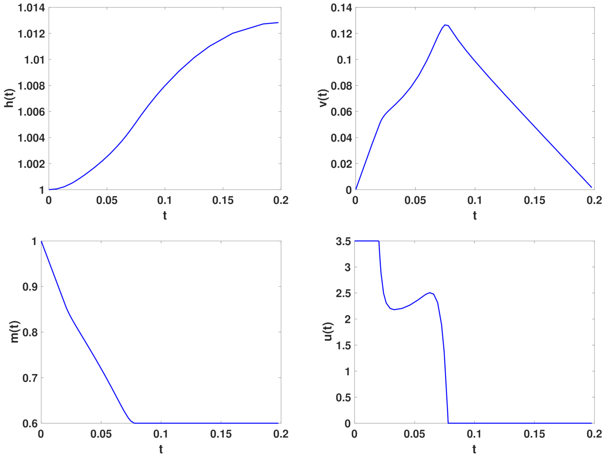
Since the problem is highly nonlinear, it is chosen as starting approximation of the solution $h={\lambda }_1={\lambda }_2={\lambda }_3=1$, ${\lambda }_4=0$, $v\left(\tau \right)=\tau (1-\tau )$, $m\left(\tau \right)=\left(m\right(1)-m(0\left)\right)\tau +m\left(0\right)$ and $T=0.01$. The choice of a good initial approximation is the main matter when the parameters of the penalty function $\overline{\sigma }$ and $ϵ$ become extremely small. In this case, it is helpful to apply a continuation strategy for the parameter $ϵ$, changing the value of this parameter from ${ϵ}_0={10}^{-1}$ to the desired value of $ϵ$. To highlight the advantages of this strategy, we solve the optimal control problem (15) choosing $\overline{\sigma }={10}^{-4}$ and two different values of $ϵ={10}^{-3},{10}^{-6}$, the solution is plotted in Figure 5.

In

Table 18. Goddard Rocket problem (15) solved using a piecewise quadratic penalty function with $\overline{\sigma }={10}^{-4}$ and $ϵ={10}^{-3}$: final mesh (fM), total number of vectorized function evaluation (NVF) and mixed errors for h, v, m, T and u.

$\mathit{t}\mathit{o}\mathit{l}={10}^{-4}$
	fM	NVF	Error h	Error v	Error m	Error T	Error u
bvp4c	1388	8058	$8.9\times {10}^{-10}$	$4.9\times {10}^{-7}$	$4.7\times {10}^{-9}$	$4.6\times {10}^{-8}$	$3.0\times {10}^{-5}$
twpbvp_m	31	86	$6.0\times {10}^{-7}$	$3.8\times {10}^{-5}$	$4.0\times {10}^{-5}$	$1.1\times {10}^{-5}$	$1.0\times {10}^{-3}$
twpbvp_l	31	91	$1.0\times {10}^{-6}$	$6.9\times {10}^{-5}$	$7.5\times {10}^{-5}$	$1.2\times {10}^{-5}$	$1.7\times {10}^{-3}$
$\mathit{t}\mathit{o}\mathit{l}={\mathbf{10}}^{-\mathbf{6}}$
bvp4c	1466	20,898	$4.9\times {10}^{-12}$	$2.7\times {10}^{-9}$	$2.6\times {10}^{-9}$	$3.1\times {10}^{-10}$	$1.7\times {10}^{-7}$
twpbvp_m	32	142	$4.6\times {10}^{-9}$	$1.6\times {10}^{-6}$	$1.5\times {10}^{-6}$	$1.4\times {10}^{-7}$	$9.8\times {10}^{-5}$
twpbvp_l	33	169	$3.7\times {10}^{-10}$	$6.8\times {10}^{-8}$	$6.5\times {10}^{-8}$	$3.3\times {10}^{-9}$	$3.9\times {10}^{-6}$

the results are computed without applying the continuation strategy, hence we observe that if on one hand only the codes bvp5c, tom and tomc fail for $ϵ={10}^{-3}$, on the other all the codes do not converge for $ϵ={10}^{-6}$. Consequently, in

Table 19. Goddard Rocket Problem (15) solved using a piecewise quadratic penalty function with $\overline{\sigma }={10}^{-4}$ and the continuation strategy: final mesh (fM), total number of vectorized function evaluation (NVF) and mixed errors for h, v, m, T and u. ${}^{*}$ Observe that acdc for $tol={10}^{-4},ϵ={10}^{-6}$ obtains a solution for $ϵ=3.98\times {10}^{-6}$.

	$\mathit{t}\mathit{o}\mathit{l}={10}^{-4}$
	$\mathbf{ϵ}={\mathbf{10}}^{-\mathbf{3}}$							$\mathbf{ϵ}={\mathbf{10}}^{-\mathbf{6}}$
	fM	NVF	Error $\mathit{h}$	Error $\mathit{v}$	Error $\mathit{m}$	Error $\mathit{T}$	Error $\mathit{u}$	fM	NVF	Error $\mathit{h}$	Error $\mathit{v}$	Error $\mathit{m}$	Error $\mathit{T}$	Error $\mathit{u}$
bvp4c	47	2823	$3.2\times {10}^{-9}$	$1.2\times {10}^{-6}$	$1.1\times {10}^{-6}$	$1.2\times {10}^{-7}$	$7.9\times {10}^{-5}$	138	46,507	$5.0\times {10}^{-9}$	$3.8\times {10}^{-7}$	$4.1\times {10}^{-7}$	$4.4\times {10}^{-8}$	$2.3\times {10}^{-3}$
twpbvp_m	16	268	$7.0\times {10}^{-7}$	$4.0\times {10}^{-5}$	$4.4\times {10}^{-5}$	$4.6\times {10}^{-6}$	$8.5\times {10}^{-4}$	93	484	$4.5\times {10}^{-9}$	$3.4\times {10}^{-5}$	$3.3\times {10}^{-5}$	$2.4\times {10}^{-7}$	$9.4\times {10}^{-2}$
twpbvp_l	16	304	$1.1\times {10}^{-6}$	$7.3\times {10}^{-5}$	$7.9\times {10}^{-5}$	$9.4\times {10}^{-6}$	$1.7\times {10}^{-3}$	225	627	$3.2\times {10}^{-9}$	$5.2\times {10}^{-7}$	$4.9\times {10}^{-7}$	$5.6\times {10}^{-8}$	$1.5\times {10}^{-3}$
tom	401	66	$1.4\times {10}^{-7}$	$6.8\times {10}^{-5}$	$6.7\times {10}^{-5}$	$1.7\times {10}^{-7}$	$4.2\times {10}^{-3}$	541	224	$1.6\times {10}^{-8}$	$3.7\times {10}^{-5}$	$3.2\times {10}^{-5}$	$1.7\times {10}^{-7}$	$4.2\times {10}^{-2}$
tomc	291	62	$5.4\times {10}^{-8}$	$3.9\times {10}^{-5}$	$3.7\times {10}^{-5}$	$8.7\times {10}^{-7}$	$2.1\times {10}^{-3}$	286	210	$1.1\times {10}^{-8}$	$9.5\times {10}^{-5}$	$9.2\times {10}^{-5}$	$8.7\times {10}^{-7}$	$1.2\times {10}^{-1}$
acdc	17	341	$7.2\times {10}^{-7}$	$8.2\times {10}^{-5}$	$8.4\times {10}^{-5}$	$9.3\times {10}^{-6}$	$5.1\times {10}^{-3}$	24 ${}^{*}$	2066	$3.8\times {10}^{-9}$	$8.7\times {10}^{-7}$	$7.1\times {10}^{-7}$	$9.2\times {10}^{-8}$	$4.8\times {10}^{-3}$
	$\mathit{t}\mathit{o}\mathit{l}={\mathbf{10}}^{-\mathbf{6}}$
bvp4c	148	9189	$3.8\times {10}^{-11}$	$7.7\times {10}^{-9}$	$6.9\times {10}^{-9}$	$9.1\times {10}^{-11}$	$8.2\times {10}^{-7}$	1385	52,028	$5.2\times {10}^{-11}$	$2.9\times {10}^{-9}$	$3.5\times {10}^{-9}$	$7.9\times {10}^{-10}$	$1.9\times {10}^{-5}$
twpbvp_m	29	593	$2.3\times {10}^{-8}$	$2.3\times {10}^{-6}$	$2.3\times {10}^{-6}$	$3.4\times {10}^{-9}$	$1.4\times {10}^{-4}$	149	681	$1.8\times {10}^{-10}$	$2.9\times {10}^{-7}$	$2.8\times {10}^{-7}$	$8.0\times {10}^{-9}$	$8.2\times {10}^{-4}$
twpbvp_l	32	646	$4.5\times {10}^{-9}$	$2.3\times {10}^{-6}$	$2.2\times {10}^{-6}$	$2.1\times {10}^{-7}$	$1.4\times {10}^{-4}$	119	969	$8.9\times {10}^{-10}$	$2.9\times {10}^{-6}$	$2.5\times {10}^{-6}$	$1.1\times {10}^{-8}$	$6.9\times {10}^{-3}$
tom	551	80	$1.6\times {10}^{-8}$	$1.4\times {10}^{-5}$	$1.4\times {10}^{-5}$	$3.0\times {10}^{-8}$	$7.3\times {10}^{-4}$	661	279	$6.3\times {10}^{-9}$	$1.7\times {10}^{-5}$	$1.5\times {10}^{-5}$	$3.0\times {10}^{-8}$	$3.5\times {10}^{-2}$
tomc	321	74	$1.1\times {10}^{-7}$	$1.7\times {10}^{-5}$	$1.6\times {10}^{-5}$	$2.4\times {10}^{-8}$	$7.7\times {10}^{-4}$	731	286	$7.3\times {10}^{-10}$	$5.6\times {10}^{-6}$	$5.4\times {10}^{-6}$	$2.4\times {10}^{-8}$	$1.2\times {10}^{-2}$
acdc	28	496	$4.5\times {10}^{-9}$	$2.3\times {10}^{-6}$	$2.2\times {10}^{-6}$	$2.1\times {10}^{-7}$	$1.4\times {10}^{-4}$	58	942	$2.3\times {10}^{-10}$	$3.5\times {10}^{-7}$	$3.4\times {10}^{-7}$	$3.5\times {10}^{-9}$	$9.7\times {10}^{-4}$

we run the codes using the continuation strategy. All the numerical tests use an initial mesh of 16 equidistant points. For the continuation strategy in Table 19, except for acdc and acdcc, the parameter $ϵ$ is initially set to ${ϵ}_0={10}^{-1}$ ( ${ϵ}_0=1$ for tom and tomc), and then it is changed using $N_{ϵ}=10$ logarithmically equispaced values up to reach the value required $ϵ$. However, to obtain the convergence of bvp4c for $ϵ={10}^{-6}$, we put the value of $N_{ϵ}=100$ when $tol={10}^{-4}$ and $N_{ϵ}=20$ when $tol={10}^{-6}$ and for tom/tomc we put the value of $N_{ϵ}=55$. The conditioning parameters reported in

Table 20. Goddard Rocket problem: conditioning parameters computed using $tol={10}^{-6}$.

	$\mathit{\sigma }$	$\mathit{\kappa }$	${\mathit{\kappa }}_1$	${\mathit{\kappa }}_2$	${\mathit{\gamma }}_1$
$ϵ={10}^{-3}$
twpbvpc_m	4.8	$9.1\times {10}^2$	$7.3\times {10}^2$	$1.8\times {10}^2$	$2.2\times {10}^2$
twpbvpc_l	4.9	$9.0\times {10}^2$	$7.2\times {10}^2$	$1.8\times {10}^2$	$2.2\times {10}^2$
tomc	5.4	$9.0\times {10}^2$	$7.3\times {10}^2$	$1.8\times {10}^2$	$1.7\times {10}^2$
$ϵ={10}^{-6}$
twpbvpc_m	5.3	$1.0\times {10}^3$	$8.2\times {10}^2$	$2.0\times {10}^2$	$2.0\times {10}^2$
twpbvpc_l	5.2	$1.0\times {10}^3$	$8.1\times {10}^2$	$2.0\times {10}^2$	$2.0\times {10}^2$
tomc	5.5	$1.0\times {10}^3$	$8.1\times {10}^2$	$2.0\times {10}^2$	$1.7\times {10}^2$

show that the problem is not stiff, but it is ill conditioned since ${\kappa }_1>{\kappa }_2$.

8. Minimization of the Fuel Cost in the Operation of a Train

As in [2,47] an optimal control problem in transportation is to minimize fuel cost in the operation of a train. To simplify the track is supposed to be straight. Let x be the position along the track measured from a fixed reference point and v the velocity of the train, such that the minimization problem is equivalent to solve the optimal control problem

$$\begin{array}{cc}\hfill \underset{v,u_a}{min}& {\int }_0^{4.8}{u}_{a}vdt,\hfill \\ \hfill x^{\prime }& =v,\hfill \\ \hfill v^{\prime }& =h\left(x\right)-F\left(v\right)+u_a-u_b,\hfill \\ \hfill 0& \le u_a\le 10,0\le u_b\le 2,\hfill \\ \hfill x\left(0\right)& =v\left(0\right)=v\left(4.8\right)=0,x\left(4.8\right)=6,\hfill \end{array}$$

(16)

where $F\left(v\right(t\left)\right)$ models the friction due to the rolling of the wheels and the air resistance and $h\left(x\right)$ is the active component of the gravitational force due to hill slopes that are respectively defined as

$$\begin{array}{cc}\hfill h\left(x\right)& {\displaystyle =\frac{2}{\pi }\left(ta{n}^{-1}\left({\displaystyle \frac{x-2}{\delta }}\right)+ta{n}^{-1}\left({\displaystyle \frac{x-4}{\delta }}\right)\right),\delta =0.05,}\hfill \\ \hfill F\left(v\right)& =0.3+0.14\left|v\right|+0.16v^2.\hfill \end{array}$$

Moreover, the control variables $u_a$ and $u_b$ represent respectively the acceleration provided by the engine and the deceleration from applying the brakes.

First, as smoothing technique let us consider piecewise quadratic penalty functions defined as

$$\begin{array}{cc}\hfill P^a(u_a;ϵ;\tau )& =\frac{ϵ}{2}{\left(u_a-5\right)}^2+\frac{1}{{\tau }^2}\left\{\begin{array}{cc}{(u_a-10+\tau )}^2\hfill & \hfill u_a>10-\tau \\ {(\tau -u_a)}^2\hfill & \hfill u_a<\tau \\ 0\hfill & \hfill \mathrm{otherwise},\end{array}\right.\hfill \\ \hfill P^b(u_b;ϵ;\tau )& =\frac{ϵ}{2}{\left(u_b-1\right)}^2+\frac{1}{{\tau }^2}\left\{\begin{array}{cc}{(u_b-2+\tau )}^2\hfill & \hfill u_b>2-\tau \\ {(\tau -u_b)}^2\hfill & \hfill u_b<\tau \\ 0\hfill & \hfill \mathrm{otherwise}.\end{array}\right.\hfill \end{array}$$

so that the Problem (16) can be written as

$$\begin{array}{cc}\hfill \underset{v,u_a}{min}& {\int }_0^{4.8}\left(u_{a}v+P^a(u_a;ϵ,\tau )+P^b(u_b;ϵ,\tau )\right)dt,\hfill \\ \hfill x^{\prime }& =v,\hfill \\ \hfill v& =h\left(x\right)-F\left(v\right)+u_a-u_b,\hfill \\ \hfill x\left(0\right)& =v\left(0\right)=v\left(4.8\right)=0,x\left(4.8\right)=6.\hfill \end{array}$$

(17)

From the Hamiltonian formulation we obtain the following BVP

$$\begin{array}{cc}\hfill x^{\prime }& =v,\hfill \\ \hfill v^{\prime }& =h\left(x\right)-F\left(v\right)+u_a-u_b,\hfill \\ \hfill {\lambda }^{\prime }& =-\mu h_x\left(x\right),\hfill \\ \hfill {\mu }^{\prime }& =-\lambda +\mu F_v\left(v\right)-u_a,\hfill \\ \hfill x\left(0\right)& =v\left(0\right)=v\left(4.8\right)=0,x\left(4.8\right)=6,\hfill \end{array}$$

(18)

where $u_a$ and $u_b$, computed by solving the equations

$$P_{u_a}^a(u_a;ϵ,\tau )+\mu +v=0,P_{u_b}^a(u_b;ϵ,\tau )-\mu =0,$$

are respectively

$$\begin{array}{cc}\hfill u_a& =\left\{\begin{array}{cc}{\displaystyle \frac{5ϵ{\tau }^2+20-2\tau -{\tau }^2(\mu +v)}{ϵ{\tau }^2+2}}\hfill & u_a>10-\tau \hfill \\ {\displaystyle \frac{\tau \left(5ϵ\tau +2-\tau (\mu +v)\right)}{ϵ{\tau }^2+2}}\hfill & u_a<\tau \hfill \\ {\displaystyle \frac{5ϵ-(\mu +v)}{ϵ}}\hfill & \mathrm{otherwise},\hfill \end{array}\right.\hfill \\ \hfill u_b& =\left\{\begin{array}{cc}{\displaystyle \frac{ϵ{\tau }^2+4-2\tau +{\tau }^2\mu }{ϵ{\tau }^2+2}}\hfill & u_b>2-\tau \hfill \\ {\displaystyle \frac{\tau \left(ϵ\tau +2+\tau \mu \right)}{ϵ{\tau }^2+2}}\hfill & u_b<\tau \hfill \\ {\displaystyle \frac{ϵ+\mu }{ϵ}}\hfill & \mathrm{otherwise}.\hfill \end{array}\right.\hfill \end{array}$$

As shown in

Table 21. Minimization of the fuel cost in the operation of a train (18) using a piecewise quadratic penalty function with $\tau ={10}^{-2}$: final mesh (fM), total number of vectorized function evaluation (NVF) and mixed errors for x, v, $u_a$, $u_b$.

	$\mathit{t}\mathit{o}\mathit{l}={10}^{-4}$
	$\mathbf{ϵ}=\mathbf{1}$						$\mathbf{ϵ}=\mathbf{0}.\mathbf{5}$
	fM	NVF	Error $\mathit{x}$	Error $\mathit{v}$	Error ${\mathit{u}}_{\mathit{a}}$	Error ${\mathit{u}}_{\mathit{b}}$	fM	NVF	Error $\mathit{x}$	Error $\mathit{v}$	Error ${\mathit{u}}_{\mathit{a}}$	Error ${\mathit{u}}_{\mathit{b}}$
bvp4c	121	1747	$3.0\times {10}^{-6}$	$6.7\times {10}^{-6}$	$3.4\times {10}^{-5}$	$1.7\times {10}^{-5}$	116	2414	$1.4\times {10}^{-6}$	$1.8\times {10}^{-6}$	$5.1\times {10}^{-5}$	$6.3\times {10}^{-5}$
bvp5c	52	3259	$9.8\times {10}^{-7}$	$5.9\times {10}^{-6}$	$3.3\times {10}^{-5}$	$1.8\times {10}^{-5}$	56	4295	$5.3\times {10}^{-7}$	$4.8\times {10}^{-6}$	$1.4\times {10}^{-4}$	$1.5\times {10}^{-4}$
twpbvp_m	34	132	$5.6\times {10}^{-6}$	$2.3\times {10}^{-5}$	$2.0\times {10}^{-4}$	$9.1\times {10}^{-5}$	52	124	$2.6\times {10}^{-2}$	$3.3\times {10}^{-2}$	$1.5\times {10}^{-2}$	$6.1\times {10}^{-3}$
twpbvpc_m	47	132	$5.7\times {10}^{-6}$	$2.3\times {10}^{-5}$	$2.0\times {10}^{-4}$	$9.1\times {10}^{-5}$	55	104	$2.6\times {10}^{-2}$	$3.3\times {10}^{-2}$	$1.5\times {10}^{-2}$	$6.2\times {10}^{-3}$
twpbvp_l	33	136	$9.0\times {10}^{-6}$	$2.8\times {10}^{-5}$	$4.3\times {10}^{-4}$	$1.0\times {10}^{-4}$	223	124	$2.2\times {10}^{-2}$	$2.6\times {10}^{-2}$	$9.9\times {10}^{-3}$	$8.7\times {10}^{-4}$
twpbvpc_l	46	136	$9.0\times {10}^{-6}$	$2.8\times {10}^{-5}$	$4.3\times {10}^{-4}$	$1.0\times {10}^{-4}$	115	104	$2.2\times {10}^{-2}$	$2.6\times {10}^{-2}$	$9.9\times {10}^{-3}$	$8.7\times {10}^{-4}$
tom	1471	44	$5.9\times {10}^{-5}$	$3.9\times {10}^{-4}$	$4.0\times {10}^{-4}$	$1.4\times {10}^{-4}$	1091	45	$4.9\times {10}^{-6}$	$2.6\times {10}^{-5}$	$1.1\times {10}^{-4}$	$8.9\times {10}^{-5}$
tomc	1406	148	$4.0\times {10}^{-7}$	$1.5\times {10}^{-6}$	$2.2\times {10}^{-5}$	$8.7\times {10}^{-6}$	2896	93	$1.2\times {10}^{-7}$	$3.7\times {10}^{-6}$	$3.5\times {10}^{-5}$	$1.5\times {10}^{-5}$

, all the methods, starting with an initial mesh of 16 equidistant points and initial solution $x=v=\lambda =\mu =1$, converge when $ϵ=1,0.5$ and $tol={10}^{-4}$.

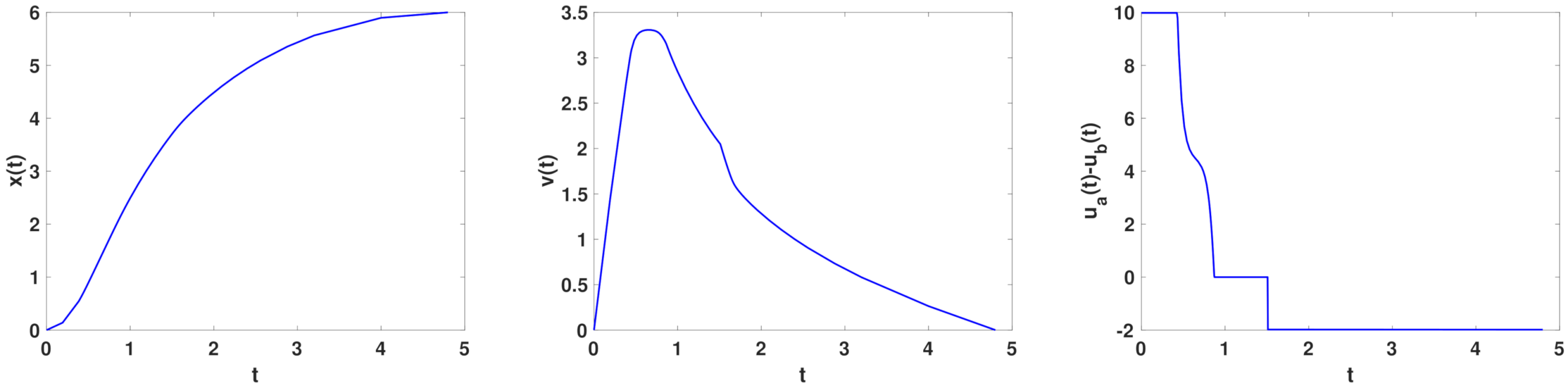
Now, decreasing the value of $ϵ$, all these methods fail, since the Problem (18) is highly ill conditioned and strongly depends on perturbations. However, these methods can reach the convergence using a continuation strategy on the parameter $ϵ$. As initial $ϵ$ we can choose 1 or 0.5, since we know that all the methods converge for those values. Moreover, we need to define the discretization for the perturbation parameter, namely we consider $N_{ϵ}$ logarithmically equispaced points in the range ${ϵ}_0$, $ϵ$. Since the continuation depends on the choice of $N_{ϵ}$ and the initial value ${ϵ}_0$, in

Table 22. Minimization of the fuel cost in the operation of a train (18) using a piecewise quadratic penalty function with $\tau ={10}^{-2}$ and continuation strategy: final mesh (fM), total number of vectorized function evaluation (NVF) and mixed errors for x, v, $u_a$, $u_b$.

	$\mathit{t}\mathit{o}\mathit{l}={10}^{-4}$
	$\mathit{ϵ}={10}^{-2}$						$\mathit{ϵ}={10}^{-3}$
	fM	NVF	Error x	Error v	Error ${\mathit{u}}_{\mathit{a}}$	Error ${\mathit{u}}_{\mathit{b}}$	fM	NVF	Error x	Error v	Error ${\mathit{u}}_{\mathit{a}}$	Error ${\mathit{u}}_{\mathit{b}}$
bvp4c	69	6055	$1.1\times {10}^{-5}$	$3.4\times {10}^{-5}$	$2.1\times {10}^{-3}$	$1.9\times {10}^{-2}$	78	8213	$1.3\times {10}^{-5}$	$3.4\times {10}^{-5}$	$5.2\times {10}^{-3}$	$1.9\times {10}^{-1}$
bvp5c	39	7180	$6.0\times {10}^{-6}$	$6.0\times {10}^{-5}$	$5.5\times {10}^{-4}$	$1.6\times {10}^{-2}$	59	8012	$1.3\times {10}^{-6}$	$5.0\times {10}^{-5}$	$6.2\times {10}^{-5}$	$1.6\times {10}^{-2}$
twpbvp_m	415	432	$4.0\times {10}^{-6}$	$7.8\times {10}^{-6}$	$1.2\times {10}^{-3}$	$4.8\times {10}^{-8}$	589	319	$4.1\times {10}^{-6}$	$9.0\times {10}^{-5}$	$2.0\times {10}^{-3}$	$2.4\times {10}^{-8}$
twpbvpc_m	132	359	$5.5\times {10}^{-5}$	$3.8\times {10}^{-4}$	$4.2\times {10}^{-3}$	$2.4\times {10}^{-2}$	589	319	$4.1\times {10}^{-6}$	$9.0\times {10}^{-5}$	$2.0\times {10}^{-3}$	$2.4\times {10}^{-8}$
twpbvp_l	202	312	$4.3\times {10}^{-5}$	$3.9\times {10}^{-4}$	$2.8\times {10}^{-3}$	$9.0\times {10}^{-3}$	589	332	$3.3\times {10}^{-6}$	$8.1\times {10}^{-5}$	$1.9\times {10}^{-3}$	$1.6\times {10}^{-8}$
twpbvpc_l	202	312	$4.3\times {10}^{-5}$	$3.9\times {10}^{-4}$	$2.8\times {10}^{-3}$	$9.0\times {10}^{-3}$	589	332	$3.3\times {10}^{-6}$	$8.1\times {10}^{-5}$	$1.9\times {10}^{-3}$	$1.6\times {10}^{-8}$
tom	2201	99	$1.5\times {10}^{-6}$	$1.2\times {10}^{-4}$	$1.7\times {10}^{-4}$	$1.3\times {10}^{-3}$	2166	102	$3.7\times {10}^{-5}$	$6.8\times {10}^{-4}$	$1.8\times {10}^{-2}$	$1.4\times {10}^{-1}$
tomc	2211	218	$4.8\times {10}^{-6}$	$1.2\times {10}^{-4}$	$1.1\times {10}^{-3}$	$5.2\times {10}^{-3}$	2886	230	$6.3\times {10}^{-6}$	$5.9\times {10}^{-5}$	$4.2\times {10}^{-3}$	$2.2\times {10}^{-1}$
acdc	36	723	$2.2\times {10}^{-6}$	$1.2\times {10}^{-5}$	$3.6\times {10}^{-4}$	$9.4\times {10}^{-3}$	40	1219	$9.4\times {10}^{-7}$	$1.7\times {10}^{-5}$	$7.6\times {10}^{-4}$	$5.2\times {10}^{-9}$

we show the results obtained using ${ϵ}_0=1$ and $N_{ϵ}=5$, except for tom/tomc for which we need to consider for the convergence $N_{ϵ}=10$. Our interest is to analyze the performance of the codes for small perturbation parameters, as $ϵ={10}^{-2},{10}^{-3}$, requiring an exit tolerance $tol={10}^{-3}$. In Figure 6 we show the solution for $ϵ={10}^{-2}$. The conditioning parameters in  

Table 23. Minimization of the fuel cost in the operation of a train: conditioning parameters computed using $tol={10}^{-6}$, cond is the condition number of the matrix associated with the last nonlinear iteration.

	$\mathit{\sigma }$	$\mathit{\kappa }$	${\mathit{\kappa }}_1$	${\mathit{\kappa }}_2$	${\mathit{\gamma }}_1$	Cond
	$ϵ={10}^{-3}$
twpbvpc_m	$6.6\times {10}^5$	$9.9\times {10}^{12}$	$9.9\times {10}^{12}$	$1.1\times {10}^3$	$1.5\times {10}^7$	$9.9\times {10}^{25}$
twpbvpc_l	$5.8\times {10}^7$	$7.3\times {10}^9$	$7.3\times {10}^9$	$7.3\times {10}^2$	$1.6\times {10}^2$	$5.3\times {10}^{19}$
tomc	$6.6\times {10}^0$	$2.8\times {10}^3$	$1.5\times {10}^3$	$1.3\times {10}^3$	$2.0\times {10}^2$	$2.4\times {10}^{15}$
	$ϵ={10}^{-6}$
twpbvpc_m	$1.1\times {10}^8$	$5.0\times {10}^{10}$	$5.0\times {10}^{10}$	$4.7\times {10}^2$	$4.9\times {10}^2$	$2.5\times {10}^{21}$
twpbvpc_l	$8.6\times {10}^7$	$7.1\times {10}^9$	$7.1\times {10}^9$	$4.7\times {10}^2$	$1.1\times {10}^2$	$5.1\times {10}^{19}$
tomc	$3.2\times {10}^0$	$1.4\times {10}^3$	$5.1\times {10}^2$	$8.9\times {10}^2$	$1.4\times {10}^2$	$2.8\times {10}^{14}$

suggest that the problem is ill conditioned but not stiff, in fact $\kappa ,{\kappa }_1,{\kappa }_2,{\gamma }_1$ are all much greater than 1. The condition number of the matrix of the last step of the integration procedure (last column of Table 23) is very high and confirms the ill-conditioning of the problem.

9. Conclusions

In this paper, after a review of general-purpose codes for solving boundary value problems we have solved some challenging optimal control problems derived using the indirect method. The presented results show that this approach could be a good alternative to the direct methods for the solution of this kind of problems, especially if the mesh selection strategy adopted is suitable for stiff problems in the case of hypersensitive problems, or an appropriate initial condition is computed for the nonlinear iteration using a continuation strategy. All these techniques can sometimes require the application of some regularization procedure, as in the presence of singular arc. Our goal with this paper is to give some indications useful to handle the input parameters of a BVP code to achieve an accurate solution, since the default values assigned usually works for very simple regular problems. Moreover, some codes give in output information about the stiffness and the conditioning of the problems, which could be used in choosing the correct solution method.

References

- Bellman, R. Dynamic Programming; Princeton University Press: Princeton, NJ, USA, 1957. [Google Scholar]
- Biral, F.; Bertolazzi, E.; Bosetti, P. Notes on Numerical Methods for Solving Optimal Control Problems. IEEE J. Ind. Appl. 2016, 5, 154–166. [Google Scholar] [CrossRef] [Green Version]
- Rao, A.V. A Survey of Numerical Methods for Optimal Control (AAS 09-334). In Astrodynamics 2009, Proceedings of the AAS/AIAA Astrodynamics Specialist Conference, Pittsburgh, PA, USA, 9–13 August 2009; American Astronautical Society by Univelt: San Diego, CA, USA, 2010; pp. 497–528. [Google Scholar]
- Soetaert, K.; Cash, J.; Mazzia, F. Solving Differential Equations in R; Springer: Berlin/Heidelberg, Germany, 2012. [Google Scholar]
- Ascher, U.; Christiansen, J.; Russell, R.D. Collocation software for boundary value odes. ACM Trans. Math. Softw. 1981, 7, 209–222. [Google Scholar] [CrossRef]
- Ascher, U.M.; Mattheij, R.M.M.; Russell, R.D. Numerical Solution of Boundary Value Problems for Ordinary Differential Equations; Classics in Applied Mathematics Series; SIAM: Philadelphia, PA, USA, 1995; Volume 13. [Google Scholar]
- Cash, J.R.; Wright, M.H. A Deferred Correction Method for Nonlinear Two-Point Boundary Value Problems: Implementation and Numerical Evaluation. SIAM J. Sci. Statist. Comput. 1991, 12, 971–989. [Google Scholar] [CrossRef]
- Bashir-Ali, Z.; Cash, J.R.; Silva, H.H.M. Lobatto deferred correction for stiff two-point boundary value problems. Comput. Math. Appl. 1998, 36, 59–69. [Google Scholar] [CrossRef] [Green Version]
- Cash, J.R.; Moore, G.; Wright, R. An automatic continuation strategy for the solution of singularly perturbed nonlinear boundary value problems. ACM Trans. Math. Softw. 2001, 27, 245–266. [Google Scholar] [CrossRef]
- Ascher, U.M.; Spiteri, R.J. Collocation software for boundary value differential-algebraic equations. SIAM J. Sci. Comput. 1994, 15, 938–952. [Google Scholar] [CrossRef]
- Enright, W.H.; Muir, P.H. Runge-Kutta software with defect control for boundary value odes. SIAM J. Sci. Comput. 1996, 17, 479–497. [Google Scholar] [CrossRef]
- Boisvert, J.J.; Muir, P.H.; Spiteri, R.J. A Runge-Kutta BVODE solver with global error and defect control. ACM Trans. Math. Softw. 2013, 39, 11. [Google Scholar] [CrossRef]
- Boisvert, J.J.; Muir, P.H.; Spiteri, R.J. BVP_SOLVER-2. Available online: https://cs.stmarys.ca/~muir/BVP_SOLVER_Webpage.shtm (accessed on 25 May 2021).
- Mazzia, F.; Cash, J.R. A Fortran test set for boundary value problem solvers. AIP Conf. Proc. 2015, 1648, 020009. [Google Scholar] [CrossRef]
- Test Set for BVP Solver. Available online: https://archimede.dm.uniba.it/~bvpsolvers/testsetbvpsolvers/?page_id=27 (accessed on 26 February 2021).
- Kierzenka, J.; Shampine, L.F. A BVP solver based on residual control and the MATLAB pse. ACM Trans. Math. Softw. 2001, 27, 299–316. [Google Scholar] [CrossRef]
- Kierzenka, J.; Shampine, L.F. A BVP solver that controls residual and error. J. Numer. Anal. Ind. Appl. Math. 2008, 3, 27–41. [Google Scholar]
- Cash, J.R.; Hollevoet, D.; Mazzia, F.; Nagy, A.M. Algorithm 927: The MATLAB Code bvptwp.m for the Numerical Solution of Two Point Boundary Value Problems. ACM Trans. Math. Softw. 2013, 39, 15. [Google Scholar] [CrossRef]
- Mazzia, F.; Sestini, A.; Trigiante, D. The continous extension of the B-spline linear multistep metods for BVPs on non-uniform meshes. Appl. Numer. Math. 2009, 59, 723–738. [Google Scholar] [CrossRef]
- Amodio, P.; Settanni, G. A finite differences MATLAB code for the numerical solution of second order singular perturbation problems. J. Comput. Appl. Math. 2012, 236, 3869–3879. [Google Scholar] [CrossRef] [Green Version]
- Auzinger, W.; Fallahpour, M.; Koch, O.; Weinmüller, E.B. Implementation of a pathfollowing strategy with an automatic step-length control: New MATLAB package bvpsuite2.0. Tech. Rep. ASC. 2019. Available online: https://www.asc.tuwien.ac.at/~ewa/software_development5.htm/ (accessed on 25 May 2021).
- Auzinger, W.; Kneisl, G.; Koch, O.; Weinmüller, E.B. A Collocation Code for Boundary Value Problems in Ordinary Differential Equations. Numer. Algorithm. 2003, 33, 27–39. [Google Scholar] [CrossRef]
- Mazzia, F.; Cash, J.R.; Soetaert, K. Solving boundary value problems in the open source software R: Package bvpSolve. Opuscula Math. 2014, 34, 387–403. [Google Scholar] [CrossRef] [Green Version]
- scipy.integrate.solve_bvp. Available online: https://docs.scipy.org/doc/scipy/reference/generated/scipy.integrate.solve_bvp.html (accessed on 25 May 2021).
- De Marinis, A.; Iavernaro, F.; Mazzia, F. A minimum-time obstacle-avoidance path planning algorithm for UAVs. Numer. Algor. 2021. [Google Scholar] [CrossRef]
- Zong, L.; Luo, J.; Wang, M. Optimal Concurrent Control for Space Manipulators Rendezvous and Capturing Targets under Actuator Saturation. IEEE Trans. Aerosp. Electron. Syst. 2020, 56, 4841–4855. [Google Scholar] [CrossRef]
- Zong, L.; Emami, M.R. Concurrent base-arm control of space manipulators with optimal rendezvous trajectory. Aerosp. Sci. Technol. 2020, 100, 105822. [Google Scholar] [CrossRef]
- Putkaradze, V.; Rogers, S. Constraint Control of Nonholonomic Mechanical Systems. J. Nonlinear Sci. 2018, 28, 193–234. [Google Scholar] [CrossRef]
- Gerdts, M. Optimal Control of ODEs and DAEs; De Gruyter Textbook: Berlin, Germany, 2012. [Google Scholar]
- Bader, G.; Ascher, U. A New Basis Implementation for a Mixed Order Boundary Value ODE Solver. SIAM J. Sci. Stat. Comput. 1987, 8, 483–500. [Google Scholar] [CrossRef]
- Capper, S.; Cash, J.; Mazzia, F. On the development of effective algorithms for the numerical solution of singularly perturbed two-point boundary value problems. Int. J. Comput. Sci. Math. 2007, 1, 42–57. [Google Scholar] [CrossRef]
- Cash, J.R.; Mazzia, F. Efficient global methods for the numerical solution of nonlinear systems of two point boundary value problems. In Recent Advances in Computational and Applied Mathematics; Simos, T., Ed.; Springer: Dordrecht, The Netherlands, 2011; pp. 23–39. [Google Scholar] [CrossRef]
- Kierzenka, J. Tutorial on Solving BVPs with BVP4C. MATLAB Central File Exchange. Available online: https://www.mathworks.com/matlabcentral/fileexchange/3819-tutorial-on-solving-bvps-with-bvp4c) (accessed on 25 February 2021).
- bvp5c. Help MATLAB. Available online: https://www.mathworks.com/help/matlab/ref/bvp5c.html (accessed on 25 February 2021).
- Brugnano, L.; Trigiante, D. Differential Problems by Multistep Initial and Boundary Value Methods; Gordon and Breach Science Publishers: Amsterdam, The Netherland, 1998. [Google Scholar]
- Mazzia, F.; Trigiante, D. A hybrid mesh selection strategy based on conditioning for boundary value ODE problems. Numer. Algorithms 2004, 36, 169–187. [Google Scholar] [CrossRef]
- Cash, J.R.; Mazzia, F. Conditioning and hybrid mesh selection algorithms for two-point boundary value problems. Scalable Comput. 2009, 10, 347–361. [Google Scholar]
- Amodio, P.; Budd, C.J.; Koch, O.; Settanni, G.; Weinmüller, E.B. Asymptotical computations for a model of flow in satured porous media. Appl. Math. Comput. 2014, 237, 155–167. [Google Scholar]
- Amodio, P.; Settanni, G. Variable-step finite difference schemes for the solution of Sturm-Liouville problems. Commun. Nonlinear Sci. 2015, 20, 641–649. [Google Scholar] [CrossRef] [Green Version]
- Amodio, P.; Settanni, G. Numerical Strategies for Solving Multiparameter Spectral Problems. In Proceedings of the Numerical Computations: Theory and Algorithms, NUMTA 2019, Crotone, Italy, 15–21 June 2019; Sergeyev, Y., Kvasov, D., Eds.; Lecture Notes in Computer Science. 2020; Volume 11974, pp. 298–305. [Google Scholar]
- Pulverer, G.; Söderlind, G.; Weinmüller, E. Automatic grid control in adaptive BVP solvers. Numer. Algorithm. 2011, 56, 61–92. [Google Scholar] [CrossRef] [Green Version]
- Rao, A.V.; Mease, K.D. Eigenvector approximate dichotomic basis method for solving hyper-sensitive optimal control problems. Optim. Control Appl. Methods 2000, 21, 1–19. [Google Scholar] [CrossRef]
- Aykutlug, E.; Topcu, U.; Mease, K.D. Manifold-Following Approximate Solution of Completely Hypersensitive Optimal Control Problems. J. Optim. Theory Appl. 2016, 170, 220–242. [Google Scholar] [CrossRef]
- ICLOCS2 (Version 2.5). Imperial College London Optimal Control Software. Available online: http://www.ee.ic.ac.uk/ICLOCS/default.htm (accessed on 2 February 2021).
- Bertolazzi, E.; Biral, F. Approximating Bang–Bang solutions in optimal control with indirect methods. In Proceedings of the Multibody Dynamics 2007, ECCOMAS Thematic Conference, Milan, Italy, 25–28 June 2007; Bottasso, C.L., Masarati, P., Trainelli, L., Eds.; Dipartimento di Ingegneria Aerospaziale, Politecnico: Milano, Italy, 2007. [Google Scholar]
- Dolan, E.D.; Moré, J.J.; Munson, T.S. Benchmarking Optimization Software with COPS 3.0; Technical Memorandum ANL/MCS-TM-273; Argonne National Laboratory, Mathematica and Computer Science, Division: Lemont, IL, USA, 2004.
- Vanderbei, R.J. Cases Studies in Trajectory Optimization: Trains, Planes, and other Pastimes. Optim. Eng. 2001, 2, 215–243. [Google Scholar] [CrossRef]
Figure 1.
Mass spring: solution in time for the mass position x on the left and the control u on the right. Final time (blue line) and (red dash-dot line).
Figure 2.
Hypersensitive: solution in time for the mass position x on the left and the control u on the right, final time .
Figure 3.
Bang-Bang, : solution in time for the mass position x on the (left), for the velocity in the (center) and the control u on the (right).
Figure 4.
Longitudinal dynamics of a vehicle, , , , , , , : theoretical (dash-dot line) and numerical (dot line) solution in time for the control u.
Figure 5.
Goddard rocket, , : from left to right solutions in time for altitude h and mass m (on the top), for velocity v and thrust u (on the bottom).