Combining Nyström Methods for a Fast Solution of Fredholm Integral Equations of the Second Kind

Abstract

In this paper, we propose a suitable combination of two different Nyström methods, both using the zeros of the same sequence of Jacobi polynomials, in order to approximate the solution of Fredholm integral equations on $[-1,1]$. The proposed procedure is cheaper than the Nyström scheme based on using only one of the described methods . Moreover, we can successfully manage functions with possible algebraic singularities at the endpoints and kernels with different pathologies. The error of the method is comparable with that of the best polynomial approximation in suitable spaces of functions, equipped with the weighted uniform norm. The convergence and the stability of the method are proved, and some numerical tests that confirm the theoretical estimates are given.

1. Introduction

Let the following be a Fredholm Integral Equation (FIE) of the second kind:

$$f\left(y\right)=g\left(y\right)+\mu {\int }_{-1}^{1}f\left(x\right)k(x,y)\rho \left(x\right)dx,y\in (-1,1),$$

(1)

where $\rho$ is a Jacobi weight, g and k are known functions defined in $(-1,1)$ and ${(-1,1)}^2$, respectively, $\mu$ is a non zero real parameter and f is the unknown function we want to look for. The kernel function k is also allowed to be weakly singular along the diagonal $y=x$, or it could show some other pathologies such as high oscillating behaviour or a “nearly singular” factor. The nature of the kernel, with the presence of the Jacobi weight inside the integral, implies that the solution f can have a singular behaviour at the endpoints of the definition interval (see for instance [1,2]); therefore, the natural choice is to study Equation (1) in suitable spaces of weighted functions.

A high number of papers on the numerical methods for FIEs is disposable in the literature, and in the last two decades a deep attention was devoted, in the case under consideration, to the so-called “global approximation methods”. They are essentially based on polynomial approximation and use zeros of orthogonal polynomials (see for instance [3,4] and the references therein). There are also examples of global approximation methods based on equispaced points [5], which are especially convenient when the data are available in discrete form but are limited to the unweighted case (see [5,6]). Global methods, more or less, behave as the best polynomial approximation of the solution in suitable spaces of weighted functions; consequently, this approximation strategy provides a powerful performance in the case of very smooth functions. On the other hand, these methods can converge slowly if the functions are not smooth or if the kernel has pathologies as described above.

Recently in [4], a new method based on the collocation approach using the so-called Extended Interpolation was proposed in order to reduce the computational effort in the cases where the solution is not so smooth [7]. Moreover the method delays the computation of high degree polynomial zeros that becomes progressively unstable as the degree increases.

Following a similar idea, we propose here a Mixed Nyström scheme based on product quadrature rules of the “extended” type, i.e., based on the zeros of the polynomial $p_{m+1}\left(w\right)p_m\left(w\right)$, where ${\left\{p_n\left(w\right)\right\}}_n$ denotes the orthonormal sequence with respect to a suitable fixed Jacobi weight w [8]. The advantages of using a Nyström scheme with respect to a collocation one include several benefits. Indeed, first of all, we will use here only one sequence of orthonormal polynomials, while in the collocation method in [4] two different sequences (${\left\{p_n\left(w\right)\right\}}_n$ and ${\left\{p_n\left({\phi }^{2}w\right)\right\}}_n$, where $\phi \left(x\right)=\sqrt{1-x^2}$) were required to obtain optimal Lebesgue constants of the interpolating operators. Secondly, due to its nature, the Nyström strategy with a fixed kernel provides a faster convergence with respect to the collocation approach if the right-hand side g in (1) is not so smooth. Third, a Nyström method based on a product rule allows treating kernel functions having different pathologies.

The idea of the proposed scheme is the following. Consider two sequences of Nyström interpolants ${\left\{f_m\right\}}_m$ and ${\left\{{\tilde{f}}_{2m+1}\right\}}_m$: The first is based on the product rule using the zeros of $p_m\left(w\right)$, and the second one is based on the extended product rule using the zeros of $p_{m+1}\left(w\right)p_m\left(w\right)$. Each step of the procedure consists in solving, for a fixed m, the first Nyström method and in using the coefficients defining the corresponding Nyström interpolant $f_m$ in order to “reduce” about one half of the computation of the coefficients of the Extended Nyström interpolant ${\tilde{f}}_{2m+1}$. In other words, we will assume that the two interpolants “coincide” on the zeros of $p_m\left(w\right)$. This assumption results in solving only a linear system of order $m+1$ instead of one of dimension $2m+1$ in order to obtain an approximating function that is comparable with ${\tilde{f}}_{2m+1}$ from the convergence point of view.

The outline of the paper is the following. Section 2 contains preliminary notations and a collection of tools needed to introduce the main results stated in Section 3. Here, we present an extended Nyström method, and the combined algorithm that allows us to solve Equation (1) faster based on this. In Section 4, we provide some computational details for the effective construction of the linear systems. Section 5 concerns the numerical tests, while Section 6 contains the proofs.

2. Notation and Preliminary Results

Throughout the paper, we use $\mathcal{C}$ in order to denote a positive constant, which may have different values at different occurrences, and we write $\mathcal{C}\ne \mathcal{C}(n,f,\dots )$ to mean that $\mathcal{C}>0$ is independent of $n,f,\dots$.

2.1. Function Spaces

Let u be the Jacobi weight defined as follows:

$$u\left(x\right)=v^{\gamma ,\delta }\left(x\right):={(1-x)}^{\gamma }{(1+x)}^{\delta },x\in (-1,1),\gamma ,\delta \ge 0.$$

We denote by $C_u$ the Banach space of the locally continuous functions f on $(-1,1)$ such that the following limit conditions are satisfied:

$$\underset{x\to 1^{-}}{lim}f\left(x\right)u\left(x\right)=0,if\gamma >0,and\underset{x\to -1^{+}}{lim}f\left(x\right)u\left(x\right)=0,if\delta >0.$$

(2)

$C_u$ is equipped with the following norm:

$${\parallel f\parallel }_{C_u}:={\parallel fu\parallel }_{\infty }=\underset{x\in [-1,1]}{max}\left|f\left(x\right)\right|u\left(x\right).$$

The limit conditions (2) are necessary in order to assure that the following is the case (see for instance [9]):

$$\underset{m\to \infty }{lim}{E}_m{\left(f\right)}_u=0,\forall f\in C_u$$

where, denoted by ${\mathbb{P}}_m$ the space of all algebraic polynomials having degree at most m, it is

$$E_m{\left(f\right)}_u:=\underset{P\in {\mathbb{P}}_m}{inf}{\parallel f-P\parallel }_{C_u}$$

the error of best polynomial approximation of $f\in C_u$.

For smoother functions, we consider the following Sobolev-type subspaces of $C_u$ of order $r\in \mathbb{N}$, defined as the following:

$$W_r\left(u\right)=\left\{f\in C_u:f^{(r-1)}\in AC\left((-1,1)\right),{\parallel f^{\left(r\right)}{\phi }^{r}u\parallel }_{\infty }<\infty \right\},r\in \mathbb{N},$$

where $AC$ denotes the space of all the functions that are absolutely continuous on every closed subset of $(-1,1)$, and $\phi \left(x\right):=\sqrt{1-x^2}$. $W_r\left(u\right)$ is equipped with the following norm:

$${\parallel f\parallel }_{W_r\left(u\right)}:={\parallel f\parallel }_{C_u}+{\parallel f^{\left(r\right)}{\phi }^{r}u\parallel }_{\infty }.$$

Finally, by $L{log}^{+}L$, we denote the set of all measurable function f defined in $(-1,1)$ such that the following is the case:

$${\int }_{-1}^1\left|f\left(x\right)\right|(1+{log}^{+}\left|f\left(x\right)\right|)dx<\infty ,{log}^{+}f\left(x\right)=log\left(max\left(1,f\left(x\right)\right)\right).$$

For any bivariate function $k(x,y)$, we will write $k_y$ (or $k_x$) in order to regard k as the univariate function in the only variable x (or y).

2.2. Solvability of the Equation (1) in $C_u$

Let us set the following:

$$\left(Kf\right)\left(y\right)=\mu {\int }_{-1}^{1}f\left(x\right)k(x,y)\rho \left(x\right)dx,\rho =v^{\sigma ,\tau },\sigma ,\tau >-1.$$

(3)

Equation (1) can be rewritten in the following form:

$$(I-K)f=g,$$

where I denotes the identity operator.

In order to provide the sufficient conditions assuring the compactness of the operator $K:C_u\to C_u$, we need to recall the following definition. For any $f\in C_u$ and with $0<r\in \mathbb{N}$, in [10], it was defined the following modulus of smoothness:

$${\Omega }_{\phi }^r{(f,t)}_u=\underset{0<h\le t}{sup}{\parallel \left({\Delta }_{h\phi }^{r}f\right)u\parallel }_{I_{hr}},$$

where

$$I_{hr}=[-1+4h^2{r}^2,1-4h^2{r}^2]$$

and the following is the case:

$${\Delta }_{h\phi }^{r}f\left(x\right)=\sum _{i=0}^r{(-1)}^i\left(\genfrac{}{}{0pt}{}{r}{i}\right)f\left(x+{\displaystyle \frac{h}{2}}(r-2i)h\phi \left(x\right)\right).$$

For any $f\in W_r\left(u\right)$, the modulus ${\Omega }_{\phi }^r{(f,t)}_u$ is estimated by means of the following inequality (see for instance [11], p. 314):

$${\Omega }_{\phi }^r{(f,t)}_u\le \mathcal{C}\underset{0<h\le t}{sup}{h}^r{\parallel f^{\left(r\right)}{\phi }^{r}u\parallel }_{I_{hr}},\mathcal{C}\ne \mathcal{C}(f,t).$$

We are now able to state a theorem that guarantees the solvability of the Equation (1) in the space $C_u$ and for which its proof is given in Section 6.

Theorem 1.

Under the following assumptions, with $0<s<r$ and $\mathcal{C}\ne \mathcal{C}\left(f\right)$,

$$\underset{\left|y\right|\le 1}{sup}\frac{k_y\rho }{u}\in L^1\left([-1,1]\right),\underset{t>0}{sup}{\displaystyle \frac{{\Omega }_{\phi }^r{(Kf,t)}_u}{t^s}}\le \mathcal{C}{\parallel f\parallel }_{C_u},$$

(4)

the operator $K:C_u\to C_u$ is compact. Therefore, if $ker(I-K)=0$, for any $g\in C_u$, Equation (1) admits a unique solution in $C_u$.

Remark 1.

We observe that (4) is satisfied also when the kernel $k(x,y)$ in (3) is weakly singular. For instance $k(x,y)={|x-y|}^{\mu },-1<\mu <0,$ fulfils the assumption with $s=1+\mu$ (see ([11], Lemma 4.1, p. 322) and ([3], pp. 3–4)).

2.3. Product Integration Rules

Denoted by ${\left\{p_m\left(w\right)\right\}}_{m\in \mathbb{N}}$, the system of the orthonormal polynomials with respect to the Jacobi weight $w=v^{\alpha ,\beta },\alpha ,\beta >-1$, the polynomial $p_m\left(w\right)$ is so defined:

$$p_m(w,x)={\gamma }_m\left(w\right)x^m+\mathrm{terms}\mathrm{of}\mathrm{lower}\mathrm{degree},{\gamma }_m\left(w\right)>0.$$

Let $\{x_k:=x_{m,k}\left(w\right):k=1,\dots ,m\}$ be the zeros of $p_m\left(w\right)$ and let the following:

$${\lambda }_{m,k}:={\lambda }_{m,k}\left(w\right)={\left(\sum _{i=0}^{m-1}{p}_i^2(w,x_k)\right)}^{-1},k=1,\dots ,m,$$

be the Christoffel numbers with respect to w.

For the following integral:

$$\mathcal{I}(f,y)={\int }_{-1}^{1}f\left(x\right)k(x,y)\rho \left(x\right)dx$$

consider the following product integration rule:

$$\mathcal{I}(f,y)=\sum _{k=1}^m{C}_k\left(y\right)f\left(x_k\right)+e_m^{\mathcal{I}}(f,y)=:{\mathcal{I}}_m(f,y)+e_m^{\mathcal{I}}(f,y),$$

(5)

where

$$C_k\left(y\right)={\lambda }_{m,k}\sum _{i=0}^{m-1}{p}_i(w,x_k)M_i\left(y\right),M_i\left(y\right)={\int }_{-1}^1{p}_i(w,x)k(x,y)\rho \left(x\right)dx,i=0,1,\cdots ,m-1.$$

(6)

According to a consolidated terminology, we will refer to the product integration rule in (5) as Ordinary Product Rule only to distinguish it from the extended product integration rule introduced below. Moreover, we recall that ${\left\{M_i\left(y\right)\right\}}_{i\in \mathbb{N}}$ are known as Modified Moments [12] (see, e.g., [13]).

With respect to the stability and the convergence of the previous rule, the following result, useful for our aim, can be deduced by ([9], p. 348) (see also [14]).

Theorem 2.

Under the following assumptions:

$$\underset{\left|y\right|\le 1}{sup}\frac{k_y\rho }{u}\in L{log}^{+}L,\underset{\left|y\right|\le 1}{sup}\frac{k_y\rho }{\sqrt{w\phi }}\in L^1\left([-1,1]\right),\frac{\sqrt{w\phi }}{u}\in L^1\left([-1,1]\right),$$

(7)

for any $f\in C_u,$ we obtain the following bounds:

$$\underset{m}{sup}\underset{\left|y\right|\le 1}{sup}\left|{\mathcal{I}}_m(f,y)\right|\le \mathcal{C}{\parallel f\parallel }_{C_u}$$

and

$$\underset{\left|y\right|\le 1}{sup}\left|e_m^{\mathcal{I}}(f,y)\right|\le \mathcal{C}{E}_{m-1}{\left(f\right)}_u,$$

with $\mathcal{C}\ne \mathcal{C}(m,f)$.

In addition to the previous well-known product rule, we recall the following Extended Product Rule (see [8]) based on the zeros of $p_m\left(w\right)p_{m+1}\left(w\right)$. Denoted by $\{y_k:=x_{m+1,k}\left(w\right):k=1,\dots ,m+1\}$ the zeros of $p_{m+1}\left(w\right)$, the extended formula is as follows: -4.6cm0cm

$$\mathcal{I}(f,y)=\sum _{k=1}^m{A}_k\left(y\right)f\left(x_k\right)+\sum _{k=1}^{m+1}{B}_k\left(y\right)f\left(y_k\right)+e_{2m+1}^{\mathsf{\Sigma }}(f,y)=:{\mathsf{\Sigma }}_{2m+1}(f,y)+e_{2m+1}^{\mathsf{\Sigma }}(f,y),$$

(8)

where

$$A_k\left(y\right)={\displaystyle \frac{{\lambda }_{m,k}}{p_{m+1}(w,x_k)}}\sum _{i=0}^{m-1}{p}_i(w,x_k)M_i^{(m+1)}\left(y\right),$$

(9)

$$B_k\left(y\right)={\displaystyle \frac{{\lambda }_{m+1,k}}{p_m(w,y_k)}}\sum _{i=0}^m{p}_i(w,y_k)M_i^{\left(m\right)}\left(y\right),$$

(10)

and

$$M_i^{\left(h\right)}\left(y\right)={\int }_{-1}^1{p}_i(w,x)p_h(w,x)k(x,y)\rho \left(x\right)dx,h\in \{m,m+1\},$$

are known as the Generalized Modified Moments (GMMs).

With respect to the stability and convergence of the extended quadrature rule (8), we recall the following.

Theorem 3

([8], Theorem 3.2). Under the following assumptions:

$$\begin{array}{c}\underset{\left|y\right|\le 1}{sup}\frac{k_y\rho }{w\phi }\in L{log}^{+}L,\underset{\left|y\right|\le 1}{sup}\frac{k_y\rho }{u}\in L^1\left([-1,1]\right),\frac{w}{u}\in L^{\infty }\left([-1,1]\right),\end{array}$$

(11)

for any $f\in C_u$, we obtain the following bounds:

$$\underset{m}{sup}\underset{\left|y\right|\le 1}{sup}\left|{\mathsf{\Sigma }}_{2m+1}(f,y)\right|\le \mathcal{C}{\parallel f\parallel }_{C_u}$$

(12)

and

$$\underset{\left|y\right|\le 1}{sup}\left|e_{2m+1}^{\mathsf{\Sigma }}(f,y)\right|\le \mathcal{C}{E}_{2m}{\left(f\right)}_u,$$

(13)

with $\mathcal{C}\ne \mathcal{C}(m,f)$.

2.4. A Nyström Method

In order to approximate the solution of (1), we recall the following weighted Nyström method based on the product quadrature rule (5). Introducing the sequence ${\left\{\left(K_{m}f\right)\left(y\right)\right\}}_m,$ where the following is the case:

$$\left(K_{m}f\right)\left(y\right)=\mu {\mathcal{I}}_m(f,y),$$

we proceed to solve in $C_u$ the following finite dimensional equation in the unknown $f_m$:

$$(I-K_m)f_m=g,m=1,2,\dots .$$

(14)

By multiplying both sides of the previous equation by the weight function u and collocating at the nodes ${\left\{x_i\right\}}_{i=1}^m$, we reach the following linear system of order m in the unknowns ${\{c_i:=f_m\left(x_i\right)u\left(x_i\right)\}}_{i=1}^m$:

$$\sum _{k=1}^m\left[{\delta }_{ik}-\mu {\displaystyle \frac{u\left(x_i\right)}{u\left(x_k\right)}}{C}_k\left(x_i\right)\right]c_k=\left(gu\right)\left(x_i\right),i=1,\dots ,m,$$

(15)

where ${\left\{C_k\left(y\right)\right\}}_k$ is defined in (6).

By setting the following:

$${\mathit{c}}_m={[c_1,\dots ,c_m]}^T,{\mathit{r}}_m={[r_1,\dots ,r_m]}^T,\mathrm{with}{r}_i=\left(gu\right)\left(x_i\right),$$

$${\mathit{D}}_m(i,k)={\delta }_{ik}-\mu {\displaystyle \frac{u\left(x_i\right)}{u\left(x_k\right)}}{C}_k\left(x_i\right),$$

the system (15) can be rewritten in the following matrix form:

$${\mathit{D}}_m{\mathit{c}}_m={\mathit{r}}_m.$$

(16)

Details on the matrix ${\mathit{D}}_m$ will be given in Section 4.

Once the solution ${\left\{c_i^{*}\right\}}_{i=1}^m$ of the system (16) has been determined, the Ordinary Nyström interpolant takes the form:

$$\left(f_{m}u\right)\left(y\right)=\left(gu\right)\left(y\right)+\mu u\left(y\right)\sum _{k=1}^m{\displaystyle \frac{c_k^{*}}{u\left(x_k\right)}}{C}_k\left(y\right).$$

(17)

About the convergence of this method, the following theorem can be obtained by using weighted arguments in [15]:

Theorem 4.

Under the assumptions of Theorems 1 and 2, for any $g\in W_r\left(u\right)$, the finite dimensional Equation (14) admits a unique solution $f_m^{*}\in C_u$ such that we have the following:

$${\parallel (f^{*}-f_m^{*})u\parallel }_{\infty }\le \mathcal{C}{\displaystyle \frac{{\parallel f\parallel }_{W_r\left(u\right)}}{m^r}},$$

(18)

with $r\ge 1$ and $\mathcal{C}\ne \mathcal{C}(m,f)$.

In what follows, we will refer to this Nyström method as the Ordinary Nyström Method (ONM).

3. Main Results

3.1. The Extended Nyström Method

Now, we introduce a Nyström method based on the extended product quadrature rule (8), calling it the Extended Nyström Method (ENM). Proceeding in analogy to the ONM, we begin by constructing the following sequence ${\left\{\left({\tilde{K}}_{2m+1}f\right)\left(y\right)\right\}}_m$:

$$\left({\tilde{K}}_{2m+1}f\right)\left(y\right)=\mu {\mathsf{\Sigma }}_{2m+1}(f,y).$$

Moreover, we solve in $C_u$ the following extended finite dimensional equation in the unknown ${\tilde{f}}_{2m+1}$:

$$(I-{\tilde{K}}_{2m+1}){\tilde{f}}_{2m+1}=g,m=1,2,\dots .$$

(19)

By multiplying both sides of (19) by the weight function u and collocating at the quadrature nodes ${\left\{x_i\right\}}_{i=1}^m\cup {\left\{y_i\right\}}_{i=1}^{m+1}$, we obtain the following linear system:

$$\left\{\begin{array}{c}{a}_i-\mu u\left(x_i\right)\left[{\displaystyle \sum _{k=1}^m}{\displaystyle \frac{a_k}{u\left(x_k\right)}}{A}_k\left(x_i\right)+{\displaystyle \sum _{k=1}^{m+1}}{\displaystyle \frac{b_k}{u\left(y_k\right)}}{B}_k\left(x_i\right)\right]=r_i,i=1,\dots ,m,\hfill \\ \\ b_i-\mu u\left(y_i\right)\left[{\displaystyle \sum _{k=1}^m}{\displaystyle \frac{a_k}{u\left(x_k\right)}}{A}_k\left(y_i\right)+{\displaystyle \sum _{k=1}^{m+1}}{\displaystyle \frac{b_k}{u\left(y_k\right)}}{B}_k\left(y_i\right)\right]=s_i,i=1,\dots ,m+1,\hfill \end{array}\right.$$

(20)

where the following is the case:

$$\begin{array}{c}{a}_i=\left({\tilde{f}}_{2m+1}u\right)\left(x_i\right),r_i=\left(gu\right)\left(x_i\right),i=1,\dots ,m,\\ b_i=\left({\tilde{f}}_{2m+1}u\right)\left(y_i\right),s_i=\left(gu\right)\left(y_i\right),i=1,\dots ,m+1.\end{array}$$

The coefficients ${\left\{A_k\left(y\right)\right\}}_{k=1}^m$ and ${\left\{B_k\left(y\right)\right\}}_{k=1}^{m+1}$ are defined in (9)–(10). The linear system of order $2m+1$ can be rewritten in the following more convenient block-matrix form:

$$\left[\begin{array}{cc}{D}_{1,1}& D_{1,2}\\ \\ D_{2,1}& D_{2,2}\end{array}\right]\left[\begin{array}{c}{\mathit{a}}_m\\ \\ {\mathit{b}}_{m+1}\end{array}\right]=\left[\begin{array}{c}{\mathit{r}}_m\\ \\ {\mathit{s}}_{m+1}\end{array}\right],$$

(21)

with $D_{1,1}\in {\mathbb{R}}^{m\times m},D_{1,2}\in {\mathbb{R}}^{m\times (m+1)},$$D_{2,1}\in {\mathbb{R}}^{(m+1)\times m}$ and $D_{2,2}\in {\mathbb{R}}^{(m+1)\times (m+1)}$. Details on the effective construction of the system will be provided in Section 4.

Denoted by ${[{{\mathit{a}}_m^{*}}^T,{{\mathit{b}}_{m+1}^{*}}^T]}^T$, the vector solution of (21), the extended Nyström interpolant takes the following form:

$$\left({\tilde{f}}_{2m+1}u\right)\left(y\right)=\left(gu\right)\left(y\right)+\mu u\left(y\right)\left[\sum _{k=1}^m{\displaystyle \frac{a_k^{*}}{u\left(x_k\right)}}{A}_k\left(y\right)+\sum _{k=1}^{m+1}{\displaystyle \frac{b_k^{*}}{u\left(y_k\right)}}{B}_k\left(y\right)\right].$$

(22)

With respect to the convergence, we are able to prove the following:

Theorem 5.

Under the assumption of Theorems 1 and 3, for any $g\in W_r\left(u\right)$, the finite dimensional Equation (19) admits a unique solution ${\tilde{f}}_{2m+1}\in C_u$ such that the following error estimate holds:

$${\parallel (f-{\tilde{f}}_{2m+1})u\parallel }_{\infty }\le \mathcal{C}{\displaystyle \frac{{\parallel f\parallel }_{W_r\left(u\right)}}{{\left(2m\right)}^r}},\mathcal{C}\ne \mathcal{C}(m,f).$$

(23)

3.2. The Mixed Nyström Method

We observe that, under suitable assumptions, both sequences ${\left\{f_m\right\}}_m$ and ${\left\{{\tilde{f}}_{2m+1}\right\}}_m$ uniformly converge to the solution f of (1). Thus, it makes sense to consider a mixed scheme that combines the two methods previously introduced.

Therefore, the Mixed Nyström Method (MNM) consists of two steps:

• For a given m, solve the linear system of order m:

  $${\mathit{D}}_m{\mathit{c}}_m={\mathit{r}}_m$$

  and construct the Nyström interpolant $f_m$ by means of its solution ${{\mathit{c}}^{*}}_m$, in other words,

  $$\left(f_{m}u\right)\left(y\right)=\left(gu\right)\left(y\right)+\mu u\left(y\right)\sum _{k=1}^m{\displaystyle \frac{c_k^{*}}{u\left(x_k\right)}}{C}_k\left(y\right).$$

  (24)
• By assuming ${\mathit{a}}_m\sim {{\mathit{c}}^{*}}_m$ in the linear system (21), we obtain the following:

  $$\begin{array}{c}\left[\begin{array}{cc}{D}_{1,1}& D_{1,2}\\ \\ D_{2,1}& D_{2,2}\end{array}\right]\left[\begin{array}{c}{{\mathit{c}}^{*}}_m\\ \\ {\tilde{\mathit{b}}}_{m+1}\end{array}\right]=\left[\begin{array}{c}{\mathit{r}}_m\\ \\ {\mathit{s}}_{m+1}\end{array}\right]\end{array}$$

  by which we deduce the reduced system of order $m+1$ in the only unknown ${\tilde{\mathit{b}}}_{m+1}$

  $$D_{2,2}{\tilde{\mathit{b}}}_{m+1}={\mathit{s}}_{m+1}-D_{2,1}{{\mathit{c}}^{*}}_m.$$

  (25)
  Denoted by ${\tilde{\mathit{b}}}_{m+1}^{*}$ its solution, we construct the interpolant ${\widehat{f}}_{2m+1}\sim {\tilde{f}}_{2m+1}$:

  $$\left({\widehat{f}}_{2m+1}u\right)\left(y\right)=\left(gu\right)\left(y\right)+\mu u\left(y\right)\left[\sum _{k=1}^m{\displaystyle \frac{c_k^{*}}{u\left(x_k\right)}}{A}_k\left(y\right)+\sum _{k=1}^{m+1}{\displaystyle \frac{{\tilde{b}}_k^{*}}{u\left(y_k\right)}}{B}_k\left(y\right)\right].$$

  (26)
• Restart the procedure determining $f_{4m}$ and ${\widehat{f}}_{8m+1}$ and so on.

The mixed sequence of Nyström interpolants is obtained by iterating a couple of steps of the types (24)–(26), allowing us to obtain the following mixed sequence of Nyström interpolants:

$${\overline{f}}_n\left(x\right)=\left\{\begin{array}{cc}{f}_{2^n}\left(x\right)\hfill & n=2,4,\dots ,\hfill \\ {\widehat{f}}_{2^n+1}\left(x\right)\hfill & n=3,5,\dots .\hfill \end{array}\right.$$

(27)

Denoting by ${\parallel A\parallel }_{\infty }={max}_{1\le i\le n}{\sum }_{j=1}^n\left|a_{ij}\right|$ the infinity norm of the matrix $A\in {\mathbb{R}}^{n\times n}$, the uniform convergence of ${\left\{{\overline{f}}_n\right\}}_n$ to the solution $f\in C_u$ of (1) is stated in the following:

Theorem 6.

Under the assumptions of Theorems 1, 4, 5 and supposing that the matrix $D_{2,2}$ in (25) is invertible, with ${sup}_n{\parallel D_{2,2}^{-1}\parallel }_{\infty }<\infty$, for any $g\in W_r\left(u\right)$, the sequence ${\left\{{\overline{f}}_n\right\}}_n$ uniformly converges to $f\in C_u$, and the following error estimate holds:

$${\parallel (f-{\overline{f}}_n)u\parallel }_{\infty }\le \mathcal{C}{\displaystyle \frac{{\parallel f\parallel }_{W_r\left(u\right)}}{{\left(2^n\right)}^r}},\mathcal{C}\ne \mathcal{C}(n,f).$$

(28)

Remark 2.

By comparing (23) with (28), both the sequences obtained by the extended and the mixed Nyström methods uniformly converge to $f\in C_u$ with the same rate of convergence.

By implementing the Mixed Nyström Method, we gain different advantages, specifically the reduction in the sizes of the involved linear systems.

More precisely, at each step of the mixed scheme, setting $m=2^n$, we solve two systems of order m and $m+1$. By doing so, the obtained error is comparable with that performed by solving the two systems of order m and $2m+1$ by the Ordinary Nyström Method.

Therefore, the computational cost of the global procedure is strongly reduced. Indeed, if we compute the solution of the linear systems by Gaussian Elimination, we save 77.8% off long operations and 33.2% off function evaluations.

Furthermore, the difficulties in the evaluation of the modified moments for “large” degree are delayed, as well as the instability in the construction of Jacobi polynomial zeros of high degrees by the Golub–Welsh algorithm.

4. Computational Details

Given two integers $h,k,h<k,$, in this section, we use the short notation $h:k$ to denote the set $h,h+1,\cdots ,k.$ Denoting by ${\mathit{I}}_m$ the identity matrix of order m, the matrix of the linear system (16) takes the following form:

$${\mathit{D}}_m:={\mathit{I}}_m-{\mathit{K}}_m,$$

with

$${\mathit{K}}_m:=\mu {\mathit{U}}_m{\mathit{M}}_m{\mathit{P}}_m{\mathsf{\Lambda }}_m{\mathit{U}}_m^{-1},$$

$$\begin{array}{c}{\mathit{U}}_m=\mathrm{diag}\left(u\left(x_1\right),\dots ,u\left(x_m\right)\right),{\mathsf{\Lambda }}_m=\mathrm{diag}\left({\lambda }_{m,1},\dots ,{\lambda }_{m,m}\right),\\ {\mathit{M}}_m(i,j)=M_j\left(x_i\right),i=1:m,j=0:m-1,\\ {\mathit{P}}_m(j,k)=p_j(w,x_k),j=0:m-1,k=1:m.\end{array}$$

It is well known that the system (16) and the finite dimensional Equation (14) are equivalent (see for instance ([16], Theorem 12.7, p. 202)).

About the block-matrix of the system (21), according to the previously introduced matrices, we have the following:

$$\begin{array}{c}{D}_{1,1}:={\mathit{I}}_m-\mu {\mathit{U}}_m{\mathit{M}}_{1,1}{\mathit{P}}_m{\mathsf{\Lambda }}_m{\mathit{Q}}_m^{-1}{\mathit{U}}_m^{-1}\in {\mathbb{R}}^{m\times m},\\ D_{1,2}:=-\mu {\mathit{U}}_m{\mathit{M}}_{1,2}{\mathit{P}}_{m+1}{\mathsf{\Lambda }}_{m+1}{\mathit{R}}_{m+1}^{-1}{\mathit{U}}_{m+1}^{-1}\in {\mathbb{R}}^{m\times (m+1)},\\ D_{2,1}:=-\mu {\mathit{U}}_{m+1}{\mathit{M}}_{2,1}{\mathit{P}}_m{\mathsf{\Lambda }}_m{\mathit{Q}}_m^{-1}{\mathit{U}}_m^{-1}\in {\mathbb{R}}^{(m+1)\times m},\\ D_{2,2}:={\mathit{I}}_{m+1}-\mu {\mathit{U}}_{m+1}{\mathit{M}}_{2,2}{\mathit{P}}_{m+1}{\mathsf{\Lambda }}_{m+1}{\mathit{R}}_{m+1}^{-1}{\mathit{U}}_{m+1}^{-1}\in {\mathbb{R}}^{(m+1)\times (m+1)},\end{array}$$

where

$$\begin{array}{c}{\mathit{Q}}_m=\mathrm{diag}\left(p_{m+1}(w,x_1),\dots ,p_{m+1}(w,x_m))\right),{\mathit{R}}_{m+1}=\mathrm{diag}\left(p_m(w,y_1),\dots ,p_m(w,y_{m+1}))\right),\\ {\mathit{U}}_{m+1}=\mathrm{diag}\left(u\left(y_1\right),\dots ,u\left(y_{m+1}\right)\right),{\mathsf{\Lambda }}_{m+1}=\mathrm{diag}\left({\mathit{\lambda }}_{m+1,1},\dots ,{\lambda }_{m+1,m+1}\right),\end{array}$$

and the matrices ${\mathit{M}}_{1,1}$, ${\mathit{M}}_{1,2}$, ${\mathit{M}}_{2,1}$ and ${\mathit{M}}_{2,2}$ are as follows:

$$\begin{array}{c}{\mathit{M}}_{1,1}(i,j)=M_j^{m+1}\left(x_i\right),i=1:m,j=0:m-1,{\mathit{M}}_{1,1}\in {\mathbb{R}}^{m\times m},\\ {\mathit{M}}_{1,2}(i,j)=M_j^m\left(x_i\right),i=1:m,j=0:m,{\mathit{M}}_{1,2}\in {\mathbb{R}}^{m\times (m+1)},\\ {\mathit{M}}_{2,1}(i,j)=M_j^{m+1}\left(y_i\right),i=1:m+1,j=0:m-1,{\mathit{M}}_{2,1}\in {\mathbb{R}}^{(m+1)\times m},\\ {\mathit{M}}_{2,2}(i,j)=M_j^m\left(y_i\right),i=1:m+1,j=0:m,{\mathit{M}}_{1,1}\in {\mathbb{R}}^{(m+1)\times (m+1)}.\end{array}$$

(29)

Remark 3.

The entries of the matrices in (29) require the computation of the GMMs. As usual, the ordinary Modified Moments (MMs), which depend on the specific kernel we considered, are often derived by suitable recurrence relations (see, e.g., [13]). In [8] a general scheme for deriving GMMs starting from MMs was proposed. Alternatively, for very smooth kernels, Gaussian rules can be also used. In any case, the global algorithm can be organized in such a manner that the matrices in (29), requiring the most expensive computation effort, can be performed once for a given couple $(m,m+1)$.

5. Numerical Experiments

Now we propose some tests showing the numerical results that were obtained by approximating the solution of equations of the type (1) by the mixed sequence ${\left\{{\overline{f}}_n\right\}}_n$ in (27). We will compare the results with those attained by the corresponding ordinary sequence used in the standard method and in Example 2 also with those achieved by the mixed collocation method proposed in [4]. Indeed, in this test, the kernel is moderately smooth, and the convergence conditions of both methods are satisfied.

We have selected g possessing different regularities and kernels k presenting some kinds of drawback such as a contemporary high oscillating behaviour with a “near” singular fixed point or being weakly singular. In each test, we will report either the common weight w used in the construction of the quadrature formulae and the weight u defining the space to which f belongs.

For effective comparison between the ordinary and the extended sequences on the same number of nodes, we have considered the following sequences:

$${\check{f}}_n\left(x\right)=\left\{\begin{array}{cc}{f}_{2^n}\left(x\right)\hfill & n=2,4,\cdots ,\hfill \\ f_{2^n+1}\left(x\right)\hfill & n=3,5,\cdots .\hfill \end{array}\right.{\overline{f}}_n\left(x\right)=\left\{\begin{array}{cc}{f}_{2^n}\left(x\right)\hfill & n=2,4,\cdots ,\hfill \\ {\widehat{f}}_{2^n+1}\left(x\right)\hfill & n=3,5,\cdots .\hfill \end{array}\right.$$

(30)

Since the solution f is unknown, we retain the exact values attained by the approximating function $f_N$, for sufficiently large N. We remark that $N=1024$ turns out to be a suitable choice for the functions under consideration. In the tables, for increasing n, we will report the weighted maximum error attained by ${\check{f}}_n$ and ${\overline{f}}_n$ at the set ${\left(z_i\right)}_{i=1,\dots ,M}$, $M=1000$ of equally spaced points of $(-1,1)$ by setting

$$E_n^{one}:=\underset{1\le i\le M}{max}|\left(u{f}_N\right)\left(z_i\right)-\left(u{\check{f}}_n\right)\left(z_i\right)|,$$

$$E_n^{mix}:=\underset{1\le i\le M}{max}|\left(u{f}_N\right)\left(z_i\right)-\left(u{\overline{f}}_n\right)\left(z_i\right)|.$$

In each table, first and third columns contain the size of the ordinary system (o.l.s.) and its condition number ${\mathrm{cond}}^{one}$ related to the ordinary sequence. In the fourth and sixth columns, the sizes of the couple of linear systems of the mixed scheme (m.l.s.) and the condition number ${\mathrm{cond}}^{mix}$ of the “reduced” system (25) are reported. All the condition numbers have been computed with respect to the infinity norm.

Finally, in order to contain possible moderate loss of accuracy in computing GMMs, we have carried out their construction by using the software Wolfram Mathematica 12.1 in quadruple precision. All the other computations have been performed in double-machine precision $eps\sim$ 2.220446049250313e-16.

Example 1.

Let us consider the following equation:

$$f\left(y\right)-\frac{1}{100\pi }{\int }_{-1}^{1}f\left(x\right){|x-y|}^{-\frac{1}{2}}{(1-x^2)}^{-\frac{1}{5}}dx={\left|y\right|}^{\frac{10}{3}}$$

$$u=v^{0.25,0.25},w=v^{0.5,0.5},\rho =v^{-0.2,-0.2}$$

In this case $g\in W_3\left(u\right)$ and according to Theorem 6, which holds since all the assumptions are satisfied, the errors are $\mathcal{O}\left(m^{-3}\right)$, and the numerical results reported in

Table 1. Example 1.

Size o.l.s.	${\mathit{E}}_{\mathit{n}}^{\mathit{one}}$	${\mathit{cond}}^{\mathit{one}}$	Size m.l.s.	${\mathit{E}}_{\mathit{n}}^{\mathit{mix}}$	${\mathit{cond}}^{\mathit{mix}}$
4	5.3 × 10−4	1.01	(4,5)	6.4 × 10−5	1.04
9	2.6 × 10−5	1.02
16	2.7 × 10−6	1.02	(16,17)	1.0 × 10−8	1.14
33	2.4 × 10−8	1.02
64	2.3 × 10−9	1.03	(64,65)	2.8 × 10−10	1.59
129	3.3 × 10−10	1.03
256	6.8 × 10−11	1.03	(256,257)	5.3 × 10−12	4.40
513	1.2 × 10−11	1.03

are even better. All the linear systems are well conditioned, the ordinary condition numbers being slightly smaller than the mixed ones. The weighted absolute errors by ONM and MNM are displayed in Figure 1.

Example 2.

Let us consider the following equation:

$$f\left(y\right)-\frac{1}{3}{\int }_{-1}^{1}f\left(x\right){|x-y|}^e{(1-x^2)}^{\frac{3}{4}}dx={\left|y\right|}^{\frac{5}{2}}$$

$$u=v^{0.7,0.7},w=\rho =v^{0.75,0.75}$$

In

Table 2. Example 2: Ordinary and Mixed Nyström methods.

Size o.l.s.	${\mathit{E}}_{\mathit{n}}^{\mathit{one}}$	${\mathit{cond}}^{\mathit{one}}$	Size m.l.s.	${\mathit{E}}_{\mathit{n}}^{\mathit{mix}}$	${\mathit{cond}}^{\mathit{mix}}$
4	1.6 × 10−4	1.99	(4,5)	8.7 × 10−5	2.60
9	2.9 × 10−5	2.07
16	4.1 × 10−6	2.13	(16,17)	1.7 × 10−7	3.03
33	4.6 × 10−7	2.13
64	4.0 × 10−8	2.13	(64,65)	1.8 × 10−9	3.10
129	4.3 × 10−9	2.14
256	3.3 × 10−10	2.14	(256,257)	1.5 × 10−11	3.11
513	3.8 × 10−11	2.14

and

Table 3. Example 2: Ordinary and Mixed Collocation methods [4].

Size o.l.s.	${\overline{\mathit{E}}}_{\mathit{n}}^{\mathit{one}}$	${\mathit{cond}}^{\mathit{one}}$	Size m.l.s.	${\overline{\mathit{E}}}_{\mathit{n}}^{\mathit{mix}}$	${\mathit{cond}}^{\mathit{mix}}$
5	1.1 × 10−2	1.99	(5,4)	1.2 × 10−2	1.31
9	3.0 × 10−3	2.07
17	7.2 × 10−4	2.13	(17,16)	1.5 × 10−3	1.45
33	1.5 × 10−4	2.13
65	3.0 × 10−5	2.13	(65,64)	2.2 × 10−5	1.52
129	5.7 × 10−6	2.14
257	9.9 × 10−7	2.14	(257,256)	8.8 × 10−8	1.52
513	1.7 × 10−7	2.14

we report the results achieved by the mixed and ordinary Nyström methods and those obtained by the mixed and ordinary collocation methods in [4]. Indeed, the assumptions assuring stability and convergence for all the methods are satisfied; hence, the comparison makes sense.

We denote by ${\overline{E}}_n^{one}$ and ${\overline{E}}_n^{mix}$ the weighted maximum error attained by the Ordinary Collocation Method (OCM) and the Mixed Collocation Method (MCM) in [4] at the set ${\left(z_i\right)}_{i=1,\dots ,M}$, $M=1000$ of equally spaced points of $(-1,1)$, respectively.

The results show that both the Nyström methods behave better than the collocation ones, and this is quite common in cases such as the one under consideration. Indeed, even if the solution $f\in W_2\left(u\right)$ (since $g\in W_2\left(u\right)$), the rate of convergence of the collocation approach depends on both the approximations of the integral operator and the right-hand side. On the contrary, the order of convergence of the Nyström method depends essentially on the smoothness of the kernel. This is one of the reasons why in these cases the Nyström approach produces better results than the collocation one, as also announced in the Introduction.

Example 3.

Let us consider the following equation:

$$f\left(y\right)-\frac{1}{2\pi }{\int }_{-1}^{1}f\left(x\right)cos\left(250x\right)\sqrt{1-x^2}dx={(1-y)}^{\frac{5}{2}}cosy$$

$$u=v^{0.1,0.1},w=\rho =v^{0.5,0.5}$$

In this test, the kernel $k(x,y)=cos\left(250x\right)$ presents a fast oscillating behaviour. Its graphic is reported in Figure 2. Hence, the product formula allows us to overcome the drawbacks deriving from the use of the Gauss–Jacobi rule. About the rate of convergence, since $g\in W_5\left(u\right)$, we expect that the errors are $\mathcal{O}\left(m^{-5}\right)$. We have reported the values attained by ONM and MNM in three different points of the interval $(-1,1)$ (

Table 4. Example 3: numerical values of the weighted solution attained by ONM and MNM.

$\mathit{x}=-0.8$
m	$\left({\check{f}}_{n}u\right)\left(x\right)$	$\left({\overline{f}}_{n}u\right)\left(x\right)$
4	2.733837532248313	2.733837532248313
9	2.733857147494405	2.733857116533352
16	2.733857151078503	2.733857151078503
33	2.733857151493599	2.733857151494889
64	2.733857151490818	2.733857151490818
129	2.733857151490921	2.733857151490937
256	2.733857151490914	2.733857151490914
513	2.733857151490910	2.733857151490910
$\mathit{x}=\mathbf{0}$
m	$\left({\check{f}}_{n}u\right)\left(x\right)$	$\left({\overline{f}}_{n}u\right)\left(x\right)$
4	9.973699234411486 × 10−1	9.97369923441148610 × 10−1
9	9.973916652404244 × 10−1	9.973916609227826 × 10−1
16	9.973916692130872 × 10−1	9.973916692130872 × 10−1
33	9.973916696731837 × 10−1	9.973916696740153 × 10−1
64	9.973916696702131 × 10−1	9.973916696702131 × 10−1
129	9.973916696702052 × 10−1	9.973916696702041 × 10−1
256	9.973916696702078 × 10−1	9.973916696702078 × 10−1
513	9.973916696702031 × 10−1	9.973916696702035 × 10−1
$\mathit{x}=\mathbf{0}.\mathbf{5}$
m	$\left({\check{f}}_{n}u\right)\left(x\right)$	$\left({\overline{f}}_{n}u\right)\left(x\right)$
4	1.502019304836581 × 10−1	1.502019304836581 × 10−1
9	1.502230544539280 × 10−1	1.502230511114784 × 10−1
16	1.502230583137010 × 10−1	1.502230583137010 × 10−1
33	1.502230587607230 × 10−1	1.502230587564985 × 10−1
64	1.502230587578369 × 10−1	1.502230587578369 × 10−1
129	1.502230587578292 × 10−1	1.502230587578573 × 10−1
256	1.502230587578317 × 10−1	1.502230587578317 × 10−1
513	1.502230587578272 × 10−1	1.502230587578276 × 10−1

) and the maximum errors on the entire interval (

Table 5. Example 3.

Size o.l.s.	${\mathit{E}}_{\mathit{n}}^{\mathit{one}}$	${\mathit{cond}}^{\mathit{one}}$	Size m.l.s.	${\mathit{E}}_{\mathit{n}}^{\mathit{mix}}$	${\mathit{cond}}^{\mathit{mix}}$
4	2.2 × 10−5	1.00	(4,5)	3.9 × 10−8	1.00
9	4.4 × 10−9	1.01
16	4.6 × 10−10	1.02	(16,17)	2.1 × 10−12	1.01
33	3.0 × 10−12	1.02
64	9.8 × 10−14	1.03	(64,65)	3.0 × 10−14	1.02
129	1.8 × 10−14	1.04
256	4.4 × 10−15	1.35	(256,257)	eps	1.31
513	4.5 × 10−16	1.36

). In all the cases the theoretical estimates are attained. Moreover, in both methods the condition numbers of the linear systems are comparable.

Example 4.

Let us consider the following equation:

$$f\left(y\right)-\frac{1}{20\pi }{\int }_{-1}^{1}f\left(x\right){\displaystyle \frac{{(1-x^2)}^{3/10}}{{(x^2+5^{-2})}^{5/4}}}dx={\left|y-\frac{1}{2}\right|}^{\frac{9}{2}}$$

$$u=v^{0.2,0.2},w=\rho =v^{0.3,0.3}$$

In this case, ρ and u satisfy the assumptions for the convergence of the Nyström methods, while they do not satisfy those of the collocation methods [4]. We recall that for the convergence of both the collocation methods smoother kernels and more restrictive assumptions on the weights are required. About the rate of convergence, since $g\in W_4\left(u\right)$, we expect that the errors are $\mathcal{O}\left(m^{-4}\right)$. Moreover, we have chosen this test to propose a comparison with the Nyström method obtained by approximating the coefficients ${\left\{C_k\left(y\right)\right\}}_{k=1}^m$ in (5) by Gaussian rules. We will refer to this procedure as the Ordinary Nyström method by Gaussian rule (shortly, ONG). We point out that the nature of the kernel k makes this comparison possible, since the computation of the coefficients by the Gauss–Jacobi rule can be performed. Thus, in

Table 6. Example 4.

Size o.l.s.	${\mathit{E}}_{\mathit{n}}^{\mathit{one}}$	${\mathit{cond}}^{\mathit{one}}$	Size m.l.s.	${\mathit{E}}_{\mathit{n}}^{\mathit{mix}}$	${\mathit{cond}}^{\mathit{mix}}$	${\mathit{E}}_{\mathit{n}}^{\mathit{ONG}}$	${\mathit{cond}}^{\mathit{ONG}}$
4	4.4 × 10−2	2.40	(4,5)	1.5 × 10−5	1.70	3.6 × 10−2	1.50
9	3.5 × 10−6	2.24				9.7 × 10−3	2.36
16	2.7 × 10−7	2.25	(16,17)	7.6 × 10−9	1.21	1.5 × 10−2	2.19
33	5.6 × 10−10	2.28				1.5 × 10−2	2.23
64	1.4 × 10−12	2.29	(64,65)	1.5 × 10−13	1.21	1.5 × 10−2	2.24
129	3.0 × 10−13	2.30				1.5 × 10−2	2.25
256	2.7 × 10−13	2.31	(256,257)	5.7 × 10−15	1.22	1.5 × 10−2	2.26
513	1.3 × 10−14	2.32				1.5 × 10−2	2.26

, in addition to the results by the mixed and ordinary Nyström methods, in the last two columns, we will set the maximum weighted errors attained by the ONG at the same set of nodes ${\left(z_i\right)}_{i=1,\dots ,M}$, $M=1000$ and the condition numbers of the corresponding linear systems. They will be shortly denoted as $E_n^{ONG}$ and ${\mathrm{cond}}^{ONG}$, respectively. The results by ONM and MNM are slightly better than the expected accuracy, and the condition numbers of the mixed linear systems are a little bit lower than their ordinary counterparts. With respect to the ONG method, as we can observe, the errors result as stagnant.

Example 5.

Let us consider the following equation:

$$f\left(y\right)-\frac{1}{27}{\int }_{-1}^{1}f\left(x\right){\displaystyle \frac{sin\left(50x\right)}{{(x^2+{50}^{-2})}^{\frac{11}{10}}}}dx=ysiny$$

$$u=v^{0,0},w=\rho =v^{0,0}$$

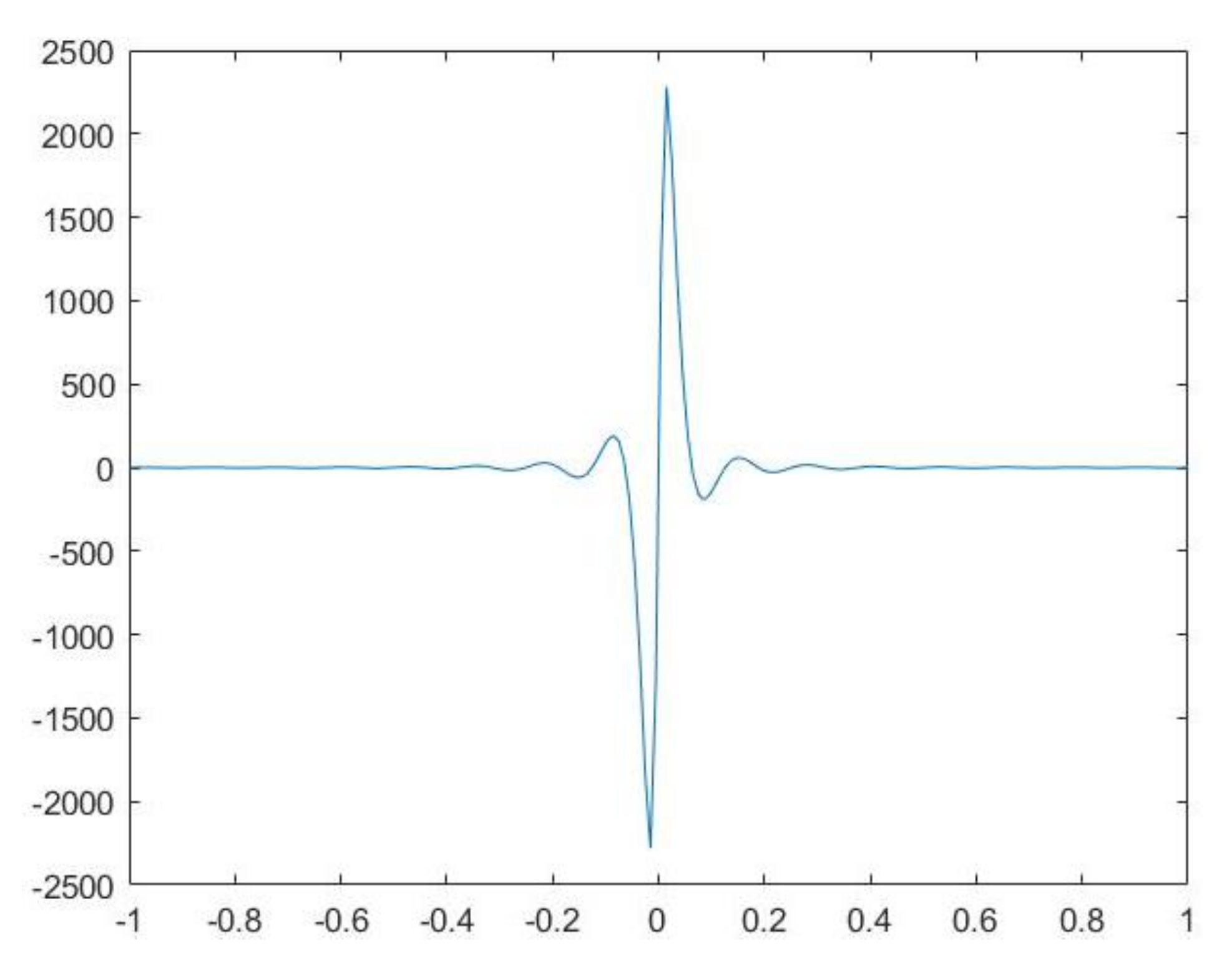
This test deals with a kernel that is a product of a periodic function having high frequency and multiplied by a “nearly” singular function. Such kernels, treated in the bidimensional case in [17], appear for instance in the solution of problems of propagation in uniform wave-guides with non-perfect conductors [18]. The graphic of the kernel is given in Figure 3. With respect to the results of the equation, since $g\in W_r\left(u\right),\forall r\ge 1$, a very fast convergence is expected, and this is confirmed also by the numerical results reported in

Table 7. Example 5.

Size o.l.s.	${\mathit{E}}_{\mathit{n}}^{\mathit{one}}$	${\mathit{cond}}^{\mathit{one}}$	Size m.l.s.	${\mathit{E}}_{\mathit{n}}^{\mathit{mix}}$	${\mathit{cond}}^{\mathit{mix}}$
4	3.9 × 10−14	1.78	(4,5)	5.5 × 10−14	1.88
9	3.3 × 10−14	3.32
16	2.0 × 10−15	5.78	(16,17)	eps	2.15
33	eps	40.9

. The mixed condition numbers are significantly smaller than the ordinary ones. The graphic of the weighted solution $fu$ is provided in Figure 4.

6. Proofs

In order to prove Theorem 1, we recall the following well-known inequality ([9], p. 171).

Proposition 1

(Weak Jackson Inequality). Let $f\in C_u$ and ${\int }_0^1\frac{{\Omega }_{\phi }^r{(f,t)}_u}{t}dt<\infty$ with $1\le r\in \mathbb{N}$. Then, the following inequality holds:

$$E_m{\left(f\right)}_u\le \mathcal{C}{\int }_0^{\frac{1}{m}}{\displaystyle \frac{{\Omega }_{\phi }^r{(f,t)}_u}{t}}dt,$$

(31)

where $m>r$ and $\mathcal{C}\ne \mathcal{C}(m,f)$.

Proof of Theorem 1.

Observing that the following is the case:

$$\left|\left(Kf\right)\left(y\right)u\left(y\right)\right|\le \left|\mu \right|u\left(y\right){\int }_{-1}^{1}f\left(x\right)k(x,y)\rho \left(x\right)dx\le {\left|\mu \right|\parallel f\parallel }_{C_u}u\left(y\right){\int }_{-1}^1\left|k(x,y)\right|{\displaystyle \frac{\rho \left(x\right)}{u\left(x\right)}}dx,$$

the boundedness of the operator K is proved by using the first assumption of (4).

A well-known result (see ([19], 2.5.1, p. 44)) states that the bounded operator K is compact if and only if $\underset{m\to +\infty }{lim}\underset{{\parallel f\parallel }_{C_u}=1}{sup}{E}_m{\left(Kf\right)}_u=0$. Then, by using the weak Jackson inequality and (4), we obtain the following bound:

$$E_m{\left(f\right)}_u\le \mathcal{C}{\int }_0^{\frac{1}{m}}{\displaystyle \frac{{\Omega }_{\phi }^r{(Kf,t)}_u}{t}}dt\le \mathcal{C}{\displaystyle \frac{{\parallel f\parallel }_{C_u}}{m^s}},\mathcal{C}\ne \mathcal{C}(m,f).$$

Thus, the theorem follows. □

To prove Theorem 5, we recall the following well-known result (see, for instance ([15], Theorem 4.1.1, p. 106)).

Theorem 7.

Let $\left(\mathcal{X},\parallel ·\parallel \right)$ be a Banach space. Assume $K:\mathcal{X}\to \mathcal{X}$ to be a bounded compact operator and $K_m:\mathcal{X}\to \mathcal{X}$, $m\in \mathbb{N}$, to be a sequence of given bounded operators with ${\displaystyle \underset{m\to \infty }{lim}\parallel Kf-K_{m}f\parallel =0}$ for all $f\in \mathcal{X}$. Consider the operator equations of the following:

$$\begin{array}{cc}\hfill (I-K)f& =g,\end{array}$$

(32)

$$\begin{array}{cc}\hfill (I-K_m)f_m& =g,\end{array}$$

(33)

where I is the identity operator in $\mathcal{X}$ and $g\in \mathcal{X}$. If ${\displaystyle \underset{m\to \infty }{lim}\parallel (K-K_m)K_m\parallel =0}$, i.e., the sequence ${\left\{K_m\right\}}_m$ is collectively compact, then , for all sufficiently large m, ${(I-K_m)}^{-1}$ exists and is uniformly bounded with the following.

$$\parallel {(I-K_m)}^{-1}\parallel \le \frac{{1+\parallel (I-K)}^{-1}\parallel \parallel K_m\parallel }{{1-\parallel (I-K)}^{-1}\parallel \parallel (K-K_m)K_m\parallel }.$$

Moreover, denoted by $f^{*}\in \mathcal{X}$ and $f_m^{*}\in \mathcal{X}$, the unique solutions of (32) and (33). respectively, the following results.

$$\parallel f^{*}-f_m^{*}\parallel \le \mathcal{C}\parallel (K-K_m)f^{*}\parallel ,\mathcal{C}\ne \mathcal{C}(m,f^{*},g).$$

Proof of Theorem 5.

The invertibility of $I-K$ follows under the assumption of Theorem 1, while the uniformly boundedness of ${\left\{{\tilde{K}}_{2m+1}\left(f\right)\right\}}_m$ and the following limit condition

$$\underset{m\to \infty }{lim}{\parallel (K-{\tilde{K}}_{2m+1})f\parallel }_{C_u}=0,\forall f\in C_u,$$

(34)

hold under the assumptions of Theorem 3.

It remains to be proven that the sequence ${\left\{{\tilde{K}}_{2m+1}\right\}}_m$ is collectively compact. This is equivalent (see ([15], p. 114) and ([19], p. 44)) to prove that $\underset{N\to +\infty }{lim}\underset{m}{sup}\underset{{\parallel f\parallel }_{C_u}=1}{sup}{E}_N{\left({\tilde{K}}_{2m+1}f\right)}_u=0$. Hence, noting that the following is the case:

$$E_N{\left({\tilde{K}}_{2m+1}f\right)}_u\le \parallel {\tilde{K}}_{2m+1}{f-P\parallel }_{C_u}\le \parallel (K-{\tilde{K}}_{2m+1}){f\parallel }_{C_u}+{\parallel Kf-P\parallel }_{C_u}$$

the thesis is easily proved using (34) and the uniform boundedness of the operator K. □

Proof of Theorem 6.

In order to prove (28), we first define the following sequence:

$${\overline{F}}_n\left(x\right)=\left\{\begin{array}{cc}{f}_{2^n}\left(x\right),\hfill & n=2,4,\cdots \hfill \\ {\tilde{f}}_{2^n+1}\left(x\right),\hfill & n=3,5,\dots \hfill \end{array}\right.$$

(35)

obtained by composing two sub-sequences of those defined by the Nyström methods ONM in (17) and ENM in (22) . As proved in Theorems 4 and 5, under the assumptions of Theorems 1, 4 and 5, these sequences are both convergent to the unique solution of the integral Equation (1). Therefore, all the sub-sequences are convergent to the same limit function f, and the speed of convergence is the same.

Consequently, we can conclude that with $m=2^n$, the following is the case:

$$\parallel [f-{\overline{F}}_n]{u\parallel }_{\infty }\le \mathcal{C}\frac{{\parallel f\parallel }_{W_r\left(u\right)}}{m^r},\mathcal{C}\ne \mathcal{C}(m,f).$$

Hence, what remain to be conducted in order to obtain (28) is to estimate the following distance:

$$\parallel [{\tilde{f}}_{2m+1}-{\widehat{f}}_{2m+1}]{u\parallel }_{\infty }.$$

From the definition of the two polynomial sequences, we can write the following:

$${\tilde{f}}_{2m+1}\left(y\right)-{\widehat{f}}_{2m+1}\left(y\right)=\mu u\left(y\right)\left[\sum _{k=1}^m{\displaystyle \frac{a_k^{*}-c_k^{*}}{u\left(x_k\right)}}{A}_k\left(y\right)+\sum _{k=1}^{m+1}{\displaystyle \frac{b_k^{*}-{\tilde{b}}_k^{*}}{u\left(y_k\right)}}{B}_k\left(y\right)\right].$$

(36)

We immediately recognize that, by the definition of ${\mathbf{a}}_m^{*}$ and ${\mathbf{c}}_m^{*}$, using estimates (18) and (23), we obtain the following.

$$\begin{array}{ccc}\hfill |a_k^{*}-c_k^{*}|& =& |{\tilde{f}}_{2m+1}\left(x_k\right)u\left(x_k\right)-f_m\left(x_k\right)u\left(x_k\right)|\hfill \\ & \le & |{\tilde{f}}_{2m+1}\left(x_k\right)u\left(x_k\right)-f\left(x_k\right)u\left(x_k\right)|+|f\left(x_k\right)u\left(x_k\right)-f_m\left(x_k\right)u\left(x_k\right)|\hfill \\ & \le & \frac{\mathcal{C}}{m^r}{\parallel f\parallel }_{W_r\left(u\right)},k=1,\dots ,m.\hfill \end{array}$$

Consequently, the following is the case:

$$\parallel {\mathbf{a}}_m^{*}-{\mathbf{c}}_m^{*}{\parallel }_{\infty }\le \frac{\mathcal{C}}{m^r}{\parallel f\parallel }_{W_r\left(u\right)},\mathcal{C}\ne \mathcal{C}(m,f),$$

(37)

where ${\parallel \mathbf{d}\parallel }_{\infty }={max}_k\left|d_k\right|$, $\mathbf{d}={[d_1,d_2,\dots ,d_m]}^T$, denotes the infinity norm in ${\mathbb{R}}^m$.

Now, we remark that by (21) and (25) and under the assumption that $D_{2,2}$ is invertible, the following identity holds true:

$$D_{2,2}({\tilde{\mathbf{b}}}_{m+1}^{*}-{\mathbf{b}}_{m+1}^{*})=D_{2,1}({\mathbf{a}}_m^{*}-{\mathbf{c}}_m^{*}).$$

Therefore, we have the following:

$$\parallel {\tilde{\mathbf{b}}}_{m+1}^{*}-{\mathbf{b}}_{m+1}^{*}{\parallel }_{\infty }\le \parallel D_{2,2}^{-1}{\parallel }_{\infty }\parallel D_{2,1}{\parallel }_{\infty }{\parallel {\mathbf{a}}_m^{*}-{\mathbf{c}}_m^{*}\parallel }_{\infty }.$$

If we denote by ${\mathcal{D}}_{2m+1}$ the matrix of coefficients in (21), we note that $D_{2,1}$ is a submatrix of it. By using standard arguments (see for instance [15]), it is possible to show that $\parallel {\mathcal{D}}_{2m+1}{\parallel }_{\infty }\le {\parallel I-{\tilde{K}}_{2m+1}\parallel }_{C_u\to C_u}$ and the operator norm at the right-hand side is uniformly bounded with respect to m since the sequence $\left\{{\tilde{K}}_{2m+1}\right\}$ is bounded in virtue of (12). Therefore, since we are assuming that ${sup}_m{\parallel D_{2,2}^{-1}\parallel }_{\infty }<\infty$, we can conclude that the following is the case:

$$\parallel {\tilde{\mathbf{b}}}_{m+1}^{*}-{\mathbf{b}}_{m+1}^{*}{\parallel }_{\infty }\le \mathcal{C}{\parallel {\mathbf{a}}_m^{*}-{\mathbf{c}}_m^{*}\parallel }_{\infty }.$$

(38)

Hence, by (36), we can obtain the following:

$$\parallel {\tilde{f}}_{2m+1}-{\widehat{f}}_{2m+1}{]u\parallel }_{\infty }\le \mathcal{C}\parallel {\mathit{a}}_m^{*}-{\mathit{c}}_m^{*}{\parallel }_{\infty }{\parallel {\tilde{K}}_{2m+1}\parallel }_{C_u\to C_u}$$

and (28) follows by (38) and estimate (12). □

7. Conclusions

In this research, we have proposed a global Nyström method involving ordinary and extended product integration rules, both based on Jacobi zeros. For the nature of the method, we can handle FIE with kernels presenting some kind of pathological behaviours since the coefficients of the rules are exactly computed via recurrence relations. The method employs two different discrete sequences, namely the ordinary and the extended sequences, that are suitably mixed to strongly reduce the computational effort required by the ordinary Nyström method. Advantages are achieved with respect to the mixed collocation method in [4] from different points of view that can be summarised as follows: we can treat FIEs as having less regular kernels and under wider assumptions in order to obtain a better rate of convergence. Such improvements have been shown by means of some numerical tests. In particular, Example 2 evidences how the mixed Nyström method provides a better performance than the mixed collocation one in [4]. Furthermore, Example 4 shows how the assumptions of the mixed Nyström method are wider than those of the above mentioned mixed collocation one. Both methods allow us to reduce the sizes of the involved linear systems but require the computation of Modified and Generalized Modified Moments. In any case, once the kernel k and the order m are given, the algorithm can be organized pre-computing the matrix of the system. Moreover, once Modified Moments are given, Generalized Modified Moments can be always deduced by a suitable recurrence relation (see, e.g., [8]). Therefore, the global process has a general applicability and only requires the assumptions of convergence to be satisfied. With respect to the Modified Moments, they can be computed through recurrence relations (see, e.g., [13]). However, when these relations are unstable, Modified Moments can be accurately computed by suitable numerical methods. For instance, in the case of high oscillating or nearly singular kernels, this approach has been successfully tried by implementing “dilation” techniques [20,21]. The major cost represents a well known limit of the classical Nyström methods based on product integration rules. They are more expensive since the coefficients of the rule possessing many and different pathological kernels have to be “exactly” computed. On the other hand, this major effort is amply repaid by the better performance with respect to other cheaper procedures. Finally, establishing that the convergence conditions are also necessary is still an open problem. This will be a subject for further investigations.

References

- Fermo, L.; Russo, M.G. Numerical methods for Fredholm integral equations with singular right-hand sides. Adv. Comput. Math. 2010, 33, 305–330. [Google Scholar] [CrossRef]
- Vainikko, G.; Pedas, A. The properties of solutions of weakly singular integral equations. J. Aust. Math. Soc. 1981, 22, 419–430. [Google Scholar] [CrossRef] [Green Version]
- De Bonis, M.C.; Mastroianni, G. Projection methods and condition numbers in uniform norm for Fredholm and Cauchy singular integral equations. SIAM J. Numer. Anal. 2006, 44, 1351–1374. [Google Scholar] [CrossRef]
- Occorsio, D.; Russo, M.G. A mixed collocation scheme for solving second kind Fredholm integral equations in [−1,1]. Electron. Trans. Numer. Anal. 2021, 54, 443–459. [Google Scholar] [CrossRef]
- Occorsio, D.; Russo, M.G. Nyström Methods for Fredholm Integral Equations Using Equispaced Points. Filomat 2014, 28, 49–63. [Google Scholar] [CrossRef]
- Occorsio, D.; Russo, M.G.; Themistoclakis, W. Some numerical applications of generalized Bernstein Operators. Constr. Math. Anal. 2021, 4, 186–214. [Google Scholar]
- Criscuolo, G.; Mastroianni, G.; Occorsio, D. Convergence of extended Lagrange interpolation. Math. Comput. 1990, 55, 197–212. [Google Scholar] [CrossRef]
- Occorsio, D.; Russo, M.G. A mixed scheme of product integration rules in (−1,1). Appl. Numer. Math. 2020, 149, 113–123. [Google Scholar] [CrossRef]
- Mastroianni, G.; Milovanović, G.V. Interpolation Processes—Basic Theory and Applications; Springer Monographs in Mathematics; Springer: Berlin, Germany, 2008. [Google Scholar]
- Ditzian, Z.; Totik, V. Moduli of Smoothness; Springer Series in Computational Mathematics; Springer: New York, NY, USA, 1987; Volume 9. [Google Scholar]
- Mastroianni, G.; Russo, M.G.; Themistoclakis, W. Numerical Methods for Cauchy Singular Integral Equations in Spaces of Weighted Continuous Functions. Oper. Theory Adv. Appl. 2005, 160, 311–336. [Google Scholar]
- Gautschi, W. On the Construction of Gaussian Quadrature Rules from Modified Moments. Math. Comput. 1970, 24, 245–260. [Google Scholar]
- Piessens, R.; Branders, M. Numerical Solution of Integral equations of Mathematical Physics using Chebyshev Polynomials. J. Comput. Phys. 1976, 21, 178–196. [Google Scholar] [CrossRef]
- Nevai, P. Mean Convergence of Lagrange Interpolation III. Trans. Am. Math. Soc. 1984, 282, 669–698. [Google Scholar] [CrossRef]
- Atkinson, K. The Numerical Solution of Integral Equations of the Second Kind; Cambridge Monographs on Applied and Computational Mathematics; Cambridge University Press: Cambridge, UK, 1997. [Google Scholar]
- Kress, R. Linear Integral Equations, 2nd ed.; Applied Mathematical Sciences; Springer: New York, NY, USA, 1999; Volume 82. [Google Scholar]
- Occorsio, D.; Serafini, G. Cubature formulae for nearly singular and highly oscillating integrals. Calcolo 2018, 55, 33. [Google Scholar] [CrossRef]
- Dobbelaere, D.; Rogier, H.; Zutter, D.D. Accurate 2.5-D boundary element method for conductive media. Radio Sci. 2014, 49, 389–399. [Google Scholar] [CrossRef] [Green Version]
- Timan, A.F. Theory of Approximation of Functions of a Real Variable; Dover Publications: New York, NY, USA, 1994. [Google Scholar]
- De Bonis, M.C.; Pastore, P. A quadrature formula for integrals of highly oscillatory functions. Rend. Circ. Mat. Palermo 2010, 2 (Suppl. 82), 279–303. [Google Scholar]
- Fermo, L.; Russo, M.G.; Serafini, G. Numerical treatment of the generalized Love integral equation. Numer. Algorithms 2021, 86, 1769–1789. [Google Scholar] [CrossRef]
Figure 1.
Example 1. (a) Errors by Ordinary Nyström Method. (b) Errors by Mixed Nyström Method.
Figure 2.
Example 3: graphic of k(x) = cos(250x).
Figure 3.
Example 5: graphic of .
Figure 4.
Example 5: graphic of the weighted solution .