
Comparison and Explanation of Forecasting Algorithms for Energy Time Series


1
Faculty of Applied Mathematics and Control Processes, Saint-Petersburg State University, Universitetskii Prospekt 35, 198504 St. Petersburg, Russia
2
Faculty of Computer Science and Technology, Saint Petersburg Electrotechnical University “LETI”, Professora Popova 5, 197376 St. Petersburg, Russia
*
Author to whom correspondence should be addressed.
Mathematics 2021, 9(21), 2794; https://0-doi-org.brum.beds.ac.uk/10.3390/math9212794
Submission received: 26 September 2021
/
Revised: 19 October 2021
/
Accepted: 29 October 2021
/
Published: 4 November 2021
(This article belongs to the Special Issue Application of Mathematical Methods in Artificial Intelligence)
Abstract
:In this work, energy time series forecasting competitions from the Schneider Company, the Kaggle Online platform, and the American society ASHRAE were considered. These competitions include power generation and building energy consumption forecasts. The datasets used in these competitions are based on reliable and real sensor records. In addition, exogenous variables are accurately added to the dataset. All of these ensure the richness of the information contained in the dataset, which is crucial for energy management. Therefore, (1) We choose to study forecast models suitable for energy management on these energy datasets; (2) Forecast models including popular algorithm structures such as neural network models and ensemble models. In addition, as an innovation, we introduce the Explainable AI method (SHAP) to explain models with excellent performance indicators, thereby strengthening its trust and transparency; (3) The results show that the performance of the integrated model in these competitions is more stable and efficient, and in the integrated model, the advantages of LightGBM are more obvious; (4) Through the interpretation of SHAP, we found that the lagging characteristics of the building area and target variables are important features.
1. Introduction
At present, models based on different algorithms are widely used in time series forecasting competitions, including the boosting algorithm [1], bagging algorithm [2] and neural network algorithm [3]. The performance of these algorithms [4] in different competitions is not stable, which means they are difficult to compare and measure. Therefore, choosing a better forecasting model by comparing different forecasting models is essential to solve the actual problems of forecasting.
Energy management systems [5] rely heavily on time series forecasting, but conventional methods cannot extract important feature information due to the complex feature composition, leading to the failure of predictive capabilities [6,7,8]. This is also the cause of the unstable performance of the forecast model on its dataset. This means that, on the one hand, we need to conduct a comprehensive comparison of popular prediction models to determine a better prediction model from a practical level. On the other hand, we need to explain the forecast model in order to have a deeper understanding of the feature information learned by the forecast model.
The energy time series forecasting competitions published by the Schneider company, the ASHRAE society and the Kaggle online platform appropriately support this work. The datasets from these competitions include both energy consumption data and solar power generation data from power plants. Importantly, the data are all reliable records from sensors, which guarantee the practical significance of the forecast model used. In addition, these competitions are time series forecasting competitions with the goal of optimizing energy management, which ensures the adaptability of our work.
In order to achieve effective measurement and comparison, both neural networks and ensemble models are considered. Among them, the neural network models Bi-RNN [9], Bi-LSTM [10], and Bi-GRU [11] are selected as representative models. The ensemble model is divided into the boosting algorithm and the bagging algorithm. The LightGBM [12] algorithm is used as the representative of the boosting algorithm, and Random Forest [13] is used as the representative of the bagging algorithm. Explainable AI technology provides a new perspective for the measurement of forecast models, and the importance of its output features can help users understand the basis of forecast models [14,15]. For example, in a field with extremely high safety requirements, such as medical care, Explainable AI technology is applied to assisted diagnosis, which is helpful for doctors to understand the analysis and recognition of pathology by algorithms, and then make correct decisions [16,17,18,19]. The popularity of machine learning and deep learning has led people to pay more attention to explainable artificial intelligence. Machine learning models and deep learning models are usually regarded as “black boxes” with internally unknown features [20,21,22]. Therefore, when applying these models, it is very important to gain people’s trust, clarify the specific meaning of their errors, and the reliability of their predictions.
In order to achieve the determination of a better forecast model, the relevant competitions information is introduced in detail in Section 2, including data description and detailed rules of the competition; in Section 3, the forecast model is introduced in detail with a pseudo code; in Section 4, the prediction results and the comparison results using classic measurement indicators are displayed. After more stable prediction models are determined, Explainable AI technology is used to explain them, so as to further determine a better forecast model.
2. Competition
2.1. Data Description
The key description in the Schneider competition is that the premise of effective operation is planning and forecasting, which means that accurate time series forecasting is absolutely needed in the energy field. At the same time, ASHRAE (American Society of Heating, Refrigerating and Air-Conditioning Engineers) pointed out in the building energy prediction competition published on Kaggle that the current estimation method is fragmented and cannot be extended well. This also leads us to be unable to determine which model is better for time series forecasting.
A description of the energy dataset used in the prediction competition is as follows:
- ASHRAE—Great Energy Predictor IIIThe dataset from ASHRAE includes the use of various energy sources in the building: chilled water, electric, hot water, and steam meters. The dataset covers more than 1000 buildings in three years. Among them, there are a total of 15 features used for prediction, including internal features such as the building id, use, area, year of completion, and floor count, as well as external features such as wind speed, wind direction, temperature, and cloud cover. The more accurate the estimation of these energy-saving investments, the more important investors, that is, financial institutions, will pay more attention to this field, thereby promoting the improvement of building efficiency. (https://www.kaggle.com/c/ashrae-energy-prediction/overview (accessed on 25 September 2021)).
- Power Laws: Forecasting Energy ConsumptionThe dataset features from Schneider include 14 features such as building id, temperature, holiday and weekend information in about 3 years. The purpose of the competition is to be able to improve the best estimate of the global consumption of buildings. (https://shop.exchange.se.com/en-US/apps/54008/forecasting-building-energy-consumption (accessed on 25 September 2021)).
- Solar Power Generation DataAs a supplement, solar power plant data was taken into account in our work. The purpose of this project is to predict the short-term solar power generation capacity for better grid management. The dataset includes five features such as device number, direct current, alternating current, temperature and radiation. (https://www.kaggle.com/anikannal/solar-power-generation-data (accessed on 25 September 2021)).
2.2. Data Visualization
In this work, the specific time point is used as the boundary between the training set and the test set, instead of rough random selection, which is more in line with the logic of the time series itself. About 70% of the elements need to be added to the training set.
- ASHRAE—Great Energy Predictor IIITaking into account the different proportions of values in different energy types, under the premise of ensuring a sufficient number of features, the meters reading of electricity type are forecasted as the target variable in this work (see Figure 1). After determining a reasonable boundary, the ratio of the training set to the test set is 0.75:0.25.
- Power Laws: Forecasting Energy ConsumptionAs shown in Figure 2, there are obvious outliers in the original data, for this reason only the data before 2014 was used in this work. After dividing by time points, the ratio of training set to test set is 0.77:0.23.
- Solar Power Generation DataUnder the condition of daily yield and total yield in the original dataset, we chose daily yield as the target variable (see Figure 3). On the one hand, considering the real-time characteristic of the forecasting model, on the other hand, the total yield can be obtained by adding the daily yield. Therefore, we are not inclined to choose total yield as the target variable. The ratio of training set to test set is 0.7:0.3.
3. Solution Approach
3.1. Known Methods
At present, in these competitions, the structures of neural networks and ensemble models are widely used. Therefore, it is necessary to select representative models in these structures to comprehensively compare the performance of forecast models. Among them, about the neural network model we choose Bi-RNN, Bi-LSTM, Bi-GRU as the representative model, in view of their higher accuracy than the unidirectional structure. The ensemble model is divided into the boosting algorithm and the bagging algorithm and we chose the Lightgbm algorithm as the representative of the boosting algorithm. In view of its excellent performance in the M5 competition, random forest is used as the representative of the bagging algorithm.
In general, in this work, LightGBM, Random Forest, Bi-RNN, Bi-LSTM and Bi-GRU are used as research objects. In addition, the version of the LightGBM model, the champion in the M5 competition [23], is directly used by us, M5 LightGBM compared with the normal version, is more applicable to complex feature structures, and the prediction effect is significantly improved.
Essentially, the ensemble model and the neural network model both deal with problems through progressive deconstruction, instead of dividing the entire dataset through complex boundaries such as support vector machines or logistic regression. Obviously, the tree-based method gradually divides the feature space along different features to optimize the information gain. What is less obvious is that neural networks also handle tasks in a similar way. Each neuron monitors a specific part of the feature space (there are multiple overlaps). When input enters this space, certain neurons will be activated. Neural networks view this piece-by-piece model fitting from a probabilistic perspective, while tree-based methods use a deterministic perspective. In any case, the performance of both depends on the depth of the model, because their components are related to various parts of the feature space.
3.2. M5 LightGBM
LightGBM is a gradient boosting framework that uses tree based learning algorithms. LightGBM optimizes the XGBoost algorithm to achieve efficient processing of large-scale data. Theoretically, the accuracy will be sacrificed while increasing the speed. However, due to the proper optimization method, the accuracy has not dropped significantly. The histogram algorithm [12] obviously improves the running speed of LightGBM.
First of all, the reduction of memory consumption caused by the histogram algorithm significantly improves the running speed of LightGBM. In this process, the memory consumption is saved by only saving discrete values of features instead of traditional pre-sorting results because the discrete value itself can store an 8-bit integer; in other words, its memory consumption can be reduced to one-eighth. On the other hand, the existence of the GOSS algorithm [12] can also ensure the balance between the speed and performance of LightGBM by means of a way that only keeps instances with more obvious gradients, but randomly samples instances with less obvious gradients. By doing this, we focus more on the under-trained instances without changing the original data distribution too much.
The M5 LightGBM version does not refer to the regression version of LightGBM (lgb.LGBMRegressor), but extracts high-quality data information through meticulous feature engineering and optimizes the parameters. Finally, an advanced version was obtained based on the traditional LightGBM (lgb.train) model. (https://github.com/Mcompetitions/M5-methods (accessed on 15 August 2021)).
3.3. Random Forest
The establishment of the Random Forest algorithm [13] is based on independent decision trees. Unlike LightGBM’s internal tree models, multiple calculation results generated by independent decision trees are integrated, and the final result is selected through a “voting” mechanism, which is the mode. On the other hand, the random sampling method ensures that it has a strong generalization ability, which also means that it can obviously control the variance of the forecasting results; however, due to the independence between decision trees, it is lacking in the ability to control variability. Therefore, the fitting effect of Random Forests will be worse, especially on datasets with large noise or datasets with a wide range of values within the feature.
3.4. Bi-RNN, Bi-LSTM, Bi-GRU
The idea of Bidirectional is to split the neurons of the traditional neural network model into two parts, one of which is responsible for the positive time direction (forward states) [9] and the other is responsible for the negative time direction (backward states) [9]. It should be noted that the output of the forward states is not connected to the input of the backward states. Compared with the traditional RNN, LSTM and GRU, the difference in Bidirectional is the addition of a backward layer.
Bi-RNN, Bi-LSTM and Bi-GRU can be seen as two layers of neural networks—the first layer from the left as the starting input of the series, in time series this can be understood as input from the beginning of time, while the second layer is from the right as the starting input, in time series processing this can be understood as input from the last time series, reversed to perform the same processing as the first layer. Finally, the two results obtained are processed.
4. Simulation Results
For calculations we used a computer with CPU—Quad-Core Intel Core i5 @ 1.4 GHz; RAM—256GB; OS—macOS Catalina 10.15.7; For implementation of the forecast models Python—JupyterLab 2.2.6 was used.
In this section, considering the simplicity, only the loss value results of the ASHRAE competition are shown as examples. Considering the computing power of the computer, we select part of the data (training set: 242214; test set: 79514) and construct a total of 98 features on this basis. The learning curve of all models showed a uniform decline (see Figure 4). Among them, the performance of the Bi-RNN validation set is even better than that of the training set. Considering the demand for comprehensive comparison, a detailed quantitative index comparison is needed.
It can be easily seen that all forecasting models have produced an excellent performance (see Figure 4 and Table 1) on ASHRAE (mainly measured from the perspective of variance), among which Bi-RNN has the best performance. However, on the other hand, the running time of M5 LightGBM is significantly less than that of random forest and neural network models, which means that in ASHRAE, M5 LightGBM can achieve an accuracy close to that of neural network models at a small time cost.
Subsequently, we continued to apply these forecasting models to different datasets, including the Schneider competition and the solar power plant dataset published on Kaggle. In the Schneider dataset, we select part of the data (training set: 271,803; test set: 78,380), and construct a total of 28 features on this basis. In the solar power dataset, we use all the data (small dataset) (Plant 1-training set: 2393; test set: 864. Plant 2-training set: 2293; test set: 862), and construct a total of 19 features on this basis.
After that, measure the performance of these forecasting models (see Table 2). On the one hand, accuracy is compared in each dataset, on the other hand, stability is compared in all datasets. Because the data values of the target variable in the Schneider and Kaggle dataset are too large, the loss optimization of all forecast models is almost invalid. Therefore, in the process of forecasting, the target variable and feature data are processed separately using the MinMax algorithm.
In the solar power datasets, for power plant 1, all forecasting models show an excellent performance (see Table 3), and M5 LightGBM is leading in terms of accuracy and time cost; for power plant 2, under the premise of maintaining high accuracy (0.9005), M5 LightGBM can still maintain the most efficient operation (see Table 4) (minimum time cost).
It can be seen from the results that M5 LightGBM has obvious advantages. From the perspective of accuracy, M5 LightGBM occupies leading positions in the two datasets (see Table 2 and Table 3), and it takes much less time than other algorithms, especially when compared with neural network algorithms. Although its performance is not the best in some datasets (see Table 1 and Table 4), the same level of forecasting performance () can still be achieved at a lower time cost. Therefore, through comprehensive comparison, we believe that M5 LightGBM is a better forecasting model. Although the idea of ensemble learning algorithm seems simple, it can often produce excellent performance in practice. This is due to the combination of multiple basic algorithm ideas that can form a reasonable framework to strengthen the advantages while weakening the weaknesses. In this way, the robustness and generalization ability of the original basic algorithm can be effectively optimized, thereby promoting the stable operation of the model.
5. Explaining the Better Forecasting Model
5.1. Explainable AI
Explainable AI strives to improve the transparency of the black box model through different approaches. At present, the more popular way is to calculate the contribution of each feature. The greater the contribution, the greater the influence on the forecasting result. At the same time, the mutual influence relationship between features can also be expressed. When the logical and common sense feature contribution is output with the forecasting result, people’s trust in the black box model will increase accordingly. It is worth noting that Explainable AI is not intended to show all the details and processes in the black box model, but to focus more on the presentation of these in a way that humans can understand.
According to the different objects that need to be explained, Explainable AI is divided into local and global. Local is the explanation of a single instance, and the global is the explanation of all datasets. For example, in a time series forecasting task, local explanation reveals how the forecast results at each point in time are affected by features (the contribution of features at each point in time), which can be applied to the real-time monitoring of time series data. The global explanation is the average degree of influence of each feature on the forecasting results in a certain period of time, which can comprehensively evaluate the black box model, so it is used as an auxiliary technology in the comparison of model performance.
According to different explanation principles, Explainable AI methods can be divided into and . refers to the model’s own explanation ability. For example, white box models, such as linear regression and decision trees, naturally belong to . On the other hand, for the black box model, Intrinsic’s purpose is to embed the explanation technology into the black box model; therefore, it is a unique explanation method for this model or this type of model, while is dedicated to the development of model-agnostic explanation methods. That is, the method that can explain all types of black box models. The main way to achieve this is to add a regular ‘perturbation’ for each feature in the dataset, and then measure the degree of change in the forecasting result (ignore the model and only focus on the forecasting result), and then calculate the contribution of the feature.
In view of the purpose of explaining the existing prediction model, we choose the SHAP [24] technology belonging to the method as the explanatory method of this work, considering that it has a theoretical system supported by cooperative games and a complete code practice tool (https://github.com/slundberg/shap, (accessed on 15 August 2021)).
5.2. Explanation Results Based on SHAP
SHAP (SHapley Additive exPlanation) is an explanation method developed based on Shapley values. It uses cooperative games as the theoretical basis, treats the black box model as a “game”, and treats each feature as a “player”. Through the calculation of the Shapley value, we can determine the contribution degree of each player (feature) in the game process (black box model operation), and then know the contribution degree of each feature.
The above is to measure the forecasting model by traditional methods, including variance and bias. In order to be able to study the interior of the model more deeply, Explainable AI technology is used by us. Originally, we were not clear about the working process of the black box model of M5 LightGBM. We could not determine which features were effectively learned by it, nor could we know the mutual influence between the internal features of the model, and so on. All of these hinder us from fully understanding the forecasting model.
In the explanation results output by SHAP (see Figure 5, Figure 6, Figure 7 and Figure 8), the transition from blue to red represents the increase in the feature value, and the SHAP value measures the impact of each feature on the model’s prediction results, and the features can be sorted according to the SHAP value. For example, in Figure 5, “square feet” is the feature with the greatest contribution, and its feature value is proportional to the target variable. In addition, the interactive results between features can show the features that have a significant impact on the feature with the greatest contribution, and use this approach to explain the interactive impact between features.
6. Conclusions
The main contribution of our work is not limited to comparing time series forecasting models in different energy data, but also includes an in-depth understanding of forecasting models from the explainable level, thereby increasing the transparency of the black box forecasting models and helping users judge whether the features learned by the model are effective. Through conventional measurement methods, we believe that M5 LightGBM is currently a better forecasting model in energy time series forecasting tasks. Through the explanation results of SHAP, we can know the contribution of each feature when M5 LightGBM is applied in specific tasks, which helps us identify important features in specific cases. Take the explanation results in this work as an example. The datasets of ASHRAE and Schneider both forecast the energy consumption of buildings. The explanation results show that their most important features are and , which are essentially the area of the building. Therefore, we believe that building area is the most important feature in building energy consumption forecasting. In addition, SHAP can also output the features that are most relevant to the most important features and the relationship between the two, which is more helpful for us to understand the internal workings of M5 LightGBM.
In the solar power data, according to the explanation result of the SHAP output, we believe that the first-order lag feature (lag 1) of the target variable is the most important feature of the solar power plant in the forecasting. This result is not only applicable to power plant 1, but the same result exists in the dataset of power plant 2; however, there are differences in the feature related to lag 1. In power plant 1, is the most relevant to power generation and is the most relevant feature in power plant 2.
In this work, the explanation is based on the global situation, and the purpose is to obtain the feature contribution over a period of time. In the future, we will pay attention to the local explanation in the time series forecasting task, that is, output the explanation results at each moment to form a real-time explanation, hoping that it can reveal the reasons for concept drift and other negative problems in time series forecasting.
Author Contributions
Investigation, K.K.; supervision, O.P.; writing–original draft, Y.Z., R.M., J.L. and X.L.; methodology, Y.Z., J.L.; software, Y.Z., R.M., J.L. and X.L.; validation, R.M., J.L., X.L.; data curation, Y.Z., R.M.; resources, Y.Z., R.M.; visualization, Y.Z., J.L., R.M. All authors have read and agreed to the published version of the manuscript.
Funding
Research funded by Ministry of Science and Higher Education of the Russian Federation (075-15-2020-93).
Institutional Review Board Statement
Not applicable.
Informed Consent Statement
Not applicable.
Acknowledgments
This work was supported by the Ministry of Science and Higher Education of the Russian Federation by the Agreement No. 075-15-2020-933 dated 13 November 2020 on the provision of a grant in the form of subsidies from the federal budget for the implementation of state support for the establishment and development of the world-class scientific center «Pavlov center» “Integrative physiology for medicine, high-tech healthcare, and stress-resilience” technologies.
Conflicts of Interest
The authors declare no conflict of interest.
References
- Robinzonov, N.; Tutz, G.; Hothorn, T. Boosting techniques for nonlinear time series models. AStA 2012, 1, 99–122. [Google Scholar] [CrossRef] [Green Version]
- Inoue, A.; Kilian, L. How useful is bagging in forecasting economic time series? A case study of US consumer price inflation. J. Am. Stat. Assoc. 2008, 482, 511–522. [Google Scholar] [CrossRef]
- Georg, D. Neural Networks for Time Series Processing. Neural Netw. World 1996, 6, 447–468. [Google Scholar]
- Zhang, Y.; Xu, F.; Zou, J.; Petrosian, O.L.; Krinkin, K.V. XAI Evaluation: Evaluating Black-Box Model Explanations for Prediction. In Proceedings of the IEEE NeuroNT, Saint Petersburg, Russia, 16 June 2021; pp. 13–16. [Google Scholar]
- Barry, P.; Prodanovic, M. State forecasting and operational planning for distribution network energy management systems. IEEE Trans. Smart Grid 2015, 7, 1002–1011. [Google Scholar]
- Chan, S.C.; Tsui, K.M.; Wu, H.C.; Hou, Y.; Wu, Y.C.; Wu, F.F. Load/price forecasting and managing demand response for smart grids: Methodologies and challenges. IEEE Signal Process. Mag. 2012, 29, 68–85. [Google Scholar] [CrossRef]
- Ghalehkhondabi, I.; Ardjm, E.; Weckman, G.R.; Young, W.A. An overview of energy demand forecasting methods published in 2005–2015. Energy Syst. 2017, 8, 411–447. [Google Scholar] [CrossRef]
- Ahmed, R.; Sreeram, V.; Mishra, Y.; Arif, M.D. A review and evaluation of the state-of-the-art in PV solar power forecasting: Techniques and optimization. RaSER 2020, 124, 109792. [Google Scholar] [CrossRef]
- Schuster, M.; Paliwal, K. Bidirectional recurrent neural networks. IEEE Trans. Signal Process. 1997, 45, 2673–2681. [Google Scholar] [CrossRef] [Green Version]
- Hochreiter, S.; Schmidhuber, J. Long short-term memory. Neural Comput. 1997, 9, 1735–1780. [Google Scholar] [CrossRef]
- Cho, K.; Van, M. Learning phrase representations using RNN encoder-decoder for statistical machine translation. arXiv 2014, arXiv:1406.1078. [Google Scholar]
- Ke, G.; Meng, Q. Lightgbm: A highly efficient gradient boosting decision tree. Neural Comput. 2017, 30, 3146–3154. [Google Scholar]
- Tin, K. The random subspace method for constructing decision forests. IEEE Trans. Pattern Anal. Mach. Intell. 1998, 20, 832–844. [Google Scholar]
- Arrieta, A. Explainable Artificial Intelligence (XAI): Concepts, taxonomies, opportunities and challenges toward responsible AI. Inf. Fusion 2020, 58, 82–115. [Google Scholar] [CrossRef] [Green Version]
- Das, A.; Rad, P. Opportunities and challenges in explainable artificial intelligence (xai): A survey. arXiv 2020, arXiv:2006.11371. [Google Scholar]
- Zou, J.; Xu, F.; Zhang, Y. High-Dimensional Explainable AI for Cancer Detection. ResearchGate. 2021. Available online: https://www.researchgate.net/publication/349715168_High-Dimensional_Explainable_AI_for_Cancer_Detection (accessed on 20 September 2021).
- Holzinger, A.; Biemann, C.; Pattichis, C.S.; Kell, D.B. What do we need to build explainable AI systems for the medical domain? arXiv 2017, arXiv:1712.09923. [Google Scholar]
- Folke, T.; Yang, S.C.H.; Anderson, S.; Shafto, P. Explainable AI for medical imaging: Explaining pneumothorax diagnoses with Bayesian teaching. arXiv 2021, arXiv:2106.04684. [Google Scholar]
- Hossain, M.; Muhammad, G.; Guizani, N. Explainable AI and mass surveillance system-based healthcare framework to combat COVID-I9 like pandemics. IEEE Netw. 2020, 34, 126–132. [Google Scholar] [CrossRef]
- Lin, Y.C.; Liang, Y.J.; Chen, M.S.; Chen, X.M. A comparative study on phenomenon and deep belief network models for hot deformation behavior of an Al-Zn-Mg-Cu alloy. Appl. Phys. Mater. Sci. Proc. 2017, 123, 68. [Google Scholar] [CrossRef]
- Lin, H.; Dai, Q.; Zheng, L.; Hong, H.; Deng, W.; Wu, F. Radial basis function artificial neural network able to accurately predict disinfection by-product levels in tap water: Taking haloacetic acids as a case study. Chemosphere 2020, 248, 125999. [Google Scholar] [CrossRef] [PubMed]
- Deng, Y.; Zhou, X.; Shen, J.; Xiao, G.; Hong, H.; Lin, H.; Liao, B.Q. New methods based on Back Propagation (BP) and Radial Basis Function (RBF) Artificial Neural Networks (ANNs) for predicting the occurrence of haloketones in tap water. Sci. Total Environ. 2021, 772, 145534. [Google Scholar] [CrossRef] [PubMed]
- Makridakis, S.; Spiliotis, E.; Assimakopoulos, V. The M5 accuracy competition: Results, findings and conclusions. Int. J. Forecast. 2020, in press. [Google Scholar] [CrossRef]
- Lundberg, S.; Lee, S. A unified approach to interpreting model predictions. In Proceedings of the 31st International Conference on Neural Information Processing Systems, Long Beach, CA, USA, 4–9 December 2017; pp. 4768–4777. [Google Scholar]
Figure 1.
The trend of the target variable of the ASHRAE.

Figure 2.
The trend of the target variable of the Power Laws.

Figure 3.
The trend of the target variable of the Solar Power Generation.

Figure 4.
ASHRAE: Learning curves of forecast models. Note: The ensemble algorithm learning curve within the LightGBM model is RMSE, and the neural network is MSE.
Figure 4.
ASHRAE: Learning curves of forecast models. Note: The ensemble algorithm learning curve within the LightGBM model is RMSE, and the neural network is MSE.

Figure 5.
ASHRAE. (Left): global explanation; (Right): inter-feature interaction. In the left figure, 1: square feet; 2: floor count 3; 3: Hour; 4: primary use Education; 5: floor count-4; 6: floor count-5; 7: primary use Entertainment; 8: floor count 6; 9: year built 1930; 10: sum of 89 other features. The global explanation result shows that “square feet” has the greatest impact on the energy consumption forecast result, and the smaller its value, the smaller the forecast value of energy consumption. Interaction result show that “wind speed” has a significant effect on “square feet”, and this effect generally occurs when “square feet” < 100,000. In this case, the existence of “wind speed” makes the influence of “square feet” on the prediction result weaker.

Figure 6.
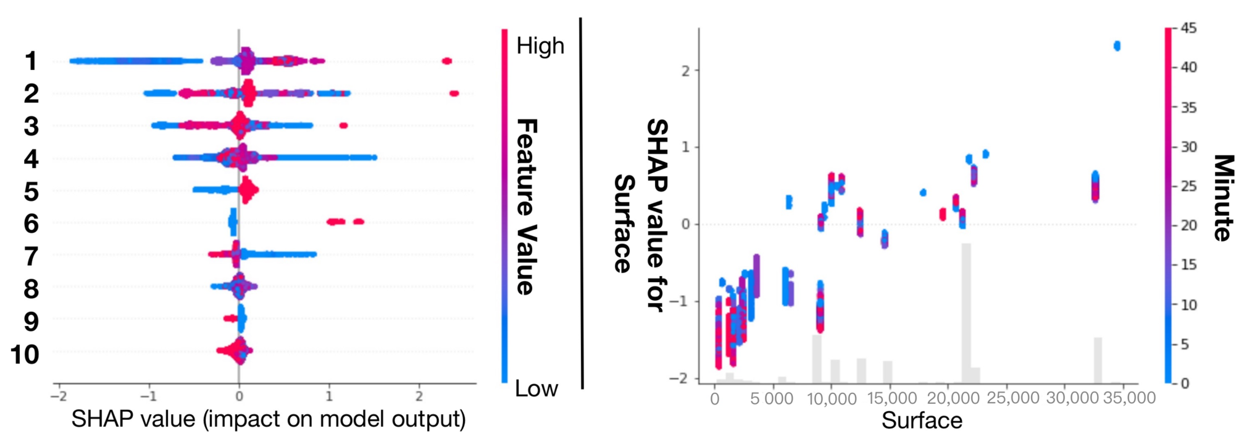
Forecasting Energy Consumption. (Left): global explanation; (Right): inter-feature interaction. In the left figure, 1: Surface; 2: SiteID; 3: ForecastID; 4: Hour; 5: Sampling 15; 6: Sampling 5; 7: Minute; 8: Month; 9: Sampling 30; 10: sum of 16 other features. The global explanation result shows that “Surface” has the greatest impact on the energy consumption forecast result, and the smaller its value, the smaller the forecast value of energy consumption. Interaction result show that “Minute” has a significant effect on “Surface”, and this effect generally occurs when “Surface” < 100,000.
Figure 6.
Forecasting Energy Consumption. (Left): global explanation; (Right): inter-feature interaction. In the left figure, 1: Surface; 2: SiteID; 3: ForecastID; 4: Hour; 5: Sampling 15; 6: Sampling 5; 7: Minute; 8: Month; 9: Sampling 30; 10: sum of 16 other features. The global explanation result shows that “Surface” has the greatest impact on the energy consumption forecast result, and the smaller its value, the smaller the forecast value of energy consumption. Interaction result show that “Minute” has a significant effect on “Surface”, and this effect generally occurs when “Surface” < 100,000.

Figure 7.
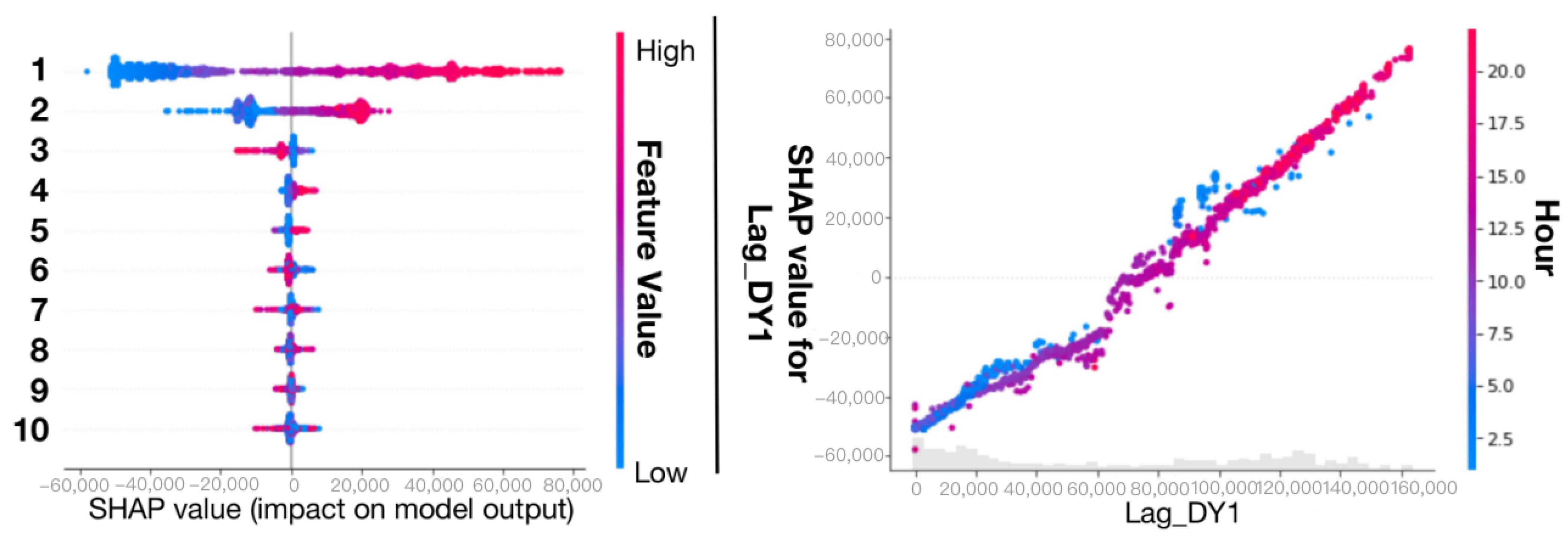
Solar Plant 1. (Left): global explanation; (Right): inter-feature interaction. In the Left figure, 1: lag DY1; 2: Hour; 3: lag DC1; 4: lag MT2; 5: lag DC2; 6: lag DY2; 7: lag AT1; 8: lag IR1; 9: lag AT2; 10: sum of 8 other features. The global explanation result shows that “lag DY1” has the greatest impact on the solar power generation result, and the smaller its value, the smaller the forecast value of solar power generation. The interaction result shows that “lag MT1” has a significant effect on “lag DY1”. At the same time, the small “lag MT1” will increase the influence of “lag DY1” on the prediction results.
Figure 7.
Solar Plant 1. (Left): global explanation; (Right): inter-feature interaction. In the Left figure, 1: lag DY1; 2: Hour; 3: lag DC1; 4: lag MT2; 5: lag DC2; 6: lag DY2; 7: lag AT1; 8: lag IR1; 9: lag AT2; 10: sum of 8 other features. The global explanation result shows that “lag DY1” has the greatest impact on the solar power generation result, and the smaller its value, the smaller the forecast value of solar power generation. The interaction result shows that “lag MT1” has a significant effect on “lag DY1”. At the same time, the small “lag MT1” will increase the influence of “lag DY1” on the prediction results.

Figure 8.
Solar Plant 2. (Left): global explanation; (Right): inter-feature interaction. In the Left figure, 1: lag DY1; 2: Hour; 3: lag DY2; 4: lag AT2; 5: lag DC1; 6: Day; 7: lag DC2; 8: lag AT1; 9: Minute; 10: sum of 8 other features. The global explanation result shows that “lag DY1” has the greatest impact on the solar power generation result, and the smaller its value, the smaller the forecast value of solar power generation. Interaction result show that “Hour” has a significant effect on “lag DY1”. At the same time, a small “Hour” will significantly weaken the influence of “lag DY1” on the prediction results, while a large “Hour” will significantly strengthen the influence of “lag DY1” on the prediction results. This means that, before noon, “lag DY1” has little effect on the prediction results, while after noon and until the evening, “lag DY1” has a significant impact on the prediction results.


Table 1.
Forecast Quality of Power ASHRAE.
| ASHRAE | |||
|---|---|---|---|
| M5LightGBM | 0.9676 | 2516.83 | 39.5 s |
| Random Forest | 0.9673 | 2538.70 | 3 min 8 s |
| Bi-RNN | 0.9688 | 2426.72 | 6 min 33 s |
| Bi-LSTM | 0.9655 | 2678.17 | 13 min 47 s |
| Bi-GRU | 0.9568 | 3358.26 | 12 min 11 s |
Table 2.
Forecast Quality of Power Schneider.
| Schneider | |||
|---|---|---|---|
| M5LightGBM | 0.9381 | 0.0001 | 42.1 s |
| Random Forest | 0.9297 | 0.0001 | 1 min 34 s |
| Bi-RNN | 0.8595 | 0.0003 | 55.2 s |
| Bi-LSTM | 0.9146 | 0.0001 | 1 min 19 s |
| Bi-GRU | 0.9165 | 0.0001 | 1 min 48 s |
Table 3.
Forecast Quality of Solar Power Generation—Plant 1.
| Plant 1 | |||
|---|---|---|---|
| M5LightGBM | 0.9928 | 0.0008 | 0.74 s |
| Random Forest | 0.9723 | 0.0034 | 0.99 s |
| Bi-RNN | 0.9665 | 0.0041 | 6.17 s |
| Bi-LSTM | 0.9887 | 0.0013 | 12.9 s |
| Bi-GRU | 0.9865 | 0.0016 | 8.36 s |
Table 4.
Forecast Quality of Solar Power Generation—Plant 2.
| Plant 2 | |||
|---|---|---|---|
| M5LightGBM | 0.9005 | 0.0081 | 0.16 s |
| Random Forest | 0.8689 | 0.0107 | 1.19 s |
| Bi-RNN | 0.9329 | 0.0055 | 6.39 s |
| Bi-LSTM | 0.8917 | 0.0088 | 13.7 s |
| Bi-GRU | 0.9185 | 0.0066 | 8.76 s |
Publisher’s Note: MDPI stays neutral with regard to jurisdictional claims in published maps and institutional affiliations. |
© 2021 by the authors. Licensee MDPI, Basel, Switzerland. This article is an open access article distributed under the terms and conditions of the Creative Commons Attribution (CC BY) license (https://creativecommons.org/licenses/by/4.0/).
Share and Cite
MDPI and ACS Style
Zhang, Y.; Ma, R.; Liu, J.; Liu, X.; Petrosian, O.; Krinkin, K. Comparison and Explanation of Forecasting Algorithms for Energy Time Series. Mathematics 2021, 9, 2794. https://0-doi-org.brum.beds.ac.uk/10.3390/math9212794
AMA Style
Zhang Y, Ma R, Liu J, Liu X, Petrosian O, Krinkin K. Comparison and Explanation of Forecasting Algorithms for Energy Time Series. Mathematics. 2021; 9(21):2794. https://0-doi-org.brum.beds.ac.uk/10.3390/math9212794
Chicago/Turabian StyleZhang, Yuyi, Ruimin Ma, Jing Liu, Xiuxiu Liu, Ovanes Petrosian, and Kirill Krinkin. 2021. "Comparison and Explanation of Forecasting Algorithms for Energy Time Series" Mathematics 9, no. 21: 2794. https://0-doi-org.brum.beds.ac.uk/10.3390/math9212794
Note that from the first issue of 2016, this journal uses article numbers instead of page numbers. See further details here.