
Mathematical and Simulation Model for Reliability Analysis of a Heterogeneous Redundant Data Transmission System †


1
Department of Applied Probability and Informatics, Peoples’ Friendship University of Russia (RUDN University), 6 Miklukho-Maklaya St, 117198 Moscow, Russia
2
V.A. Trapeznikov Institute of Control Sciences of Russian Academy of Sciences, 65 Profsoyuznaya Street, 117997 Moscow, Russia
*
Author to whom correspondence should be addressed.
†
This paper is an extended version of our paper published in 2020 IEEE 12th International Congress on Ultra-Modern Telecommunications and Control Systems and Workshops (ICUMT), Brno, Czech Republic, 5–7 October 2020, pp. 189–194, doi:10.1109/ICUMT51630.2020.9222431.
Mathematics 2021, 9(22), 2884; https://0-doi-org.brum.beds.ac.uk/10.3390/math9222884
Submission received: 24 September 2021
/
Revised: 3 November 2021
/
Accepted: 4 November 2021
/
Published: 12 November 2021
(This article belongs to the Special Issue Stochastic Modeling and Applied Probability)
Abstract
:In the actual study, we carried out a reliability analysis of a repairable redundant data transmission system with the use of the elaborated mathematical and simulation model of a closed heterogeneous cold standby system. The system consists of one repair unit and two different data sources with an exponential cumulative distribution function (CDF) of their uptime and a general independent CDF of their repair time. We consider five special cases of the general independent CDF; including Gamma, Weibull-Gnedenko, Exponential, Lognormal and Pareto. We study the system-level reliability, defined as the steady-state probability (SSP) of failure-free system operation. The proposed analytical methodology made it possible to assess the reliability of the whole system in the event of failure of its components. Specific analytic expressions and asymptotic valuations are obtained for the steady-state probabilities of the system and the SSP of failure-free system operation. A simulation model of the system in cases where it is not workable to obtain expressions for the steady-state probabilities of the system in an explicit analytical form was considered, in particular for constructing the empirical system reliability function. The issue of sensitivity analysis of reliability characteristics of the considered system to the types of repair time distributions was also studied. The simulation modeling was done with the R statistics package.
1. Introduction
Today, the methods of applied probability theory, stochastic processes, mathematical statistics, stochastic analysis, and queuing theory contribute to the resolution of the most complex problems, among which we can note the modern communication networks. The solution to these problems is to improve the availability and reliability of data transmission systems such as wireless communication networks. Today’s wireless networks will reach a remarkable level of performance and efficiency in the years to come thanks to the progress of new mathematical models. One of the principal directions of creating the ultra-high-speed and reliable wireless communications within the framework of the development of future generation networks is the development of hybrid redundant systems based on laser and radio technologies, each of which is sensitive to certain environmental conditions. A feature of such redundancy is that harsh weather conditions for one of the data transmissions channels do not affect the performance of the other channel. One of the main conditions for stable operation of the data transmission system is the insensitivity of quality and effectiveness of the system to the changes in the initial parameters of the model. The analysis of such sensitivity, which was carried out within the framework of this study, is one of the new areas of research of highly reliable next-generation data transmission systems, and it extends the previous studies in this area [1].
Previously [2], we performed the reliability assessment for a redundant system with arbitrary input distributions using the simulation model. In addition, we obtained the values of the relative repair rate at which the desired level of reliability is achieved, and presented plots of the system uptime probability and plots of the empirical distribution function and the empirical reliability function.
In [3], the simulation approach was used to investigate the reliability of a homogeneous warm-standby data transmission system. Relative recovery rate (RRR) values at which the desired level of reliability is achieved were obtained with a relatively small excess of the mean availability values over the value of the repair time. A graphical analysis of the results obtained showed high asymptotic insensitivity of the empirical CDF and the system reliability function to the input distributions. In [4,5], it has been shown, respectively, that it is not always possible to obtain explicit analytical expressions for the SSP distribution of the homogeneous restorable data transmission system with hot and cold backup. The simulation model elaborated in this work made it possible to study the reliability at the system level, which is defined as the SSP of failure-free system operations, and also to assess the system reliability characteristics.
In [6], authors used the theory of uncertainty to study the mean time to failure (MTTF) and the reliability functions of the general system, within the framework of the reliability analysis of general systems with bi-uncertain variables. Using independent and non-identical uncertainty distributions with uncertain parameters for the lifetimes of system components, they presented the explicit expressions of the MTTF and the reliability function of each model. They also established and analyzed basic models of general systems with bi-uncertain variables. Authors of [7] carried out a mathematical model, using partial differential equations to investigate the reliability of a two-component parallel repairable system with vacation. They assumed that component life follows exponential distribution and that component repair time and repairer’s vacation time have general distribution, while the repairer goes on a vacation at the start. In [8], authors focused on the reliability analysis of a cold standby system under stepwise Poisson shocks, which come with intensity depending on the number of failures of the working element. They obtained an important reliability index for the system, using the supplementary variable method and the vector Markov process theory. Either internal factors or external shocks led to the system failure. Repair after breakage was assumed imperfect. In [9,10], authors investigated a reliability model of repairable systems with stochastic lifetimes and uncertain repair times. They established, respectively, the mathematical models of the reliability of repairable series systems/parallel/series-parallel/parallel-series systems. Li, J.; Chen, Y.; Yong, Z.; and Hung, H., [11] studied an availability model for a periodic inspection system with different lifetimes and repair-time distributions. They proposed an analytical and probabilistic model of availability for the considered system, using a new recursive algorithm that can provide limited average availability and instantaneous availability of a periodical inspection system with an arbitrary distribution of service life and repair time. Their approach can provide the technology support for improving system availability and determining a reasonable inspection period. Liu B.-y.; Feng Q.; Liu S.-q.; and Cai S.-w. [12], examined a reliability model with applications for calibration data. They developed a Wiener process model for modeling the calibration data by obtaining the unknown parameters of the model using the maximum likelihood estimation approach. Lutfiah I. and Al T. [13] investigated the characteristics and application of the non-homogeneous Poisson process (NHPP) log-logistic reliability model. An NHPP reliability model based on the two-parameter log-logistic (LL) distribution was considered. Wang C. [14] investigated an approximate reliability analysis of large heterogeneous cold-standby systems. Abbas B.; Javad B.; and Tore M. [15] demonstrated the application of the available reliability models with covariates in the field of spare part predictions by means of a case study.
Furthermore, in other articles, it was reported that the use of one server and two identical units of the cold standby system with an imperfect switch is considered a semi-Markov process with three states. Such as in [16], Khorshidian, K. and Fathizadeh, M. explored an alternative approach to the reliability analysis of cold standby systems. Parshutina, S. and Bogatyrev, V. [17], demonstrated possibilities of the developed simulation models and means to support the computer-aided design of highly reliable distributed computer systems. The, J.; Lai, C.-M.; and Cheng, Y.-H. [18] presented a transmission line failure model and examined the effects of its parameters and the impact of the weather data correlation on the reliability performance of the considered system. Lisnianski, A.; Laredo, D.; and Haim, H.B. [19] performed a reliability analysis of a combined cycle gas turbine power plant by the means of a multi-state Markov model. Sensitivity analysis for reliability data uncertainty was also provided. Additionally, in [20,21,22], other authors have respectively focused their work on a “reliability analysis of cold standby compound system”, “reliability analysis of a cold standby system attacked by shocks” and a “reliability analysis of a renewable multiple cold standby system”.
In the present article, we continue to perform the reliability study of a closed heterogeneous cold standby data transmission system with only one repair unit, with two different unreliable data sources, with an exponential CDF of uptime and a general independent CDF of the repair time of its components using the analytical approach [23]. System components (data sources) are subject to failure with different rates. Failures of system components are of a binary nature and can lead to different states of the system. Same as in the series of our previous works, in the current study we use the so-called Markovization method, which consists of introducing a supplementary variable that allows description of the behavior of the considered system by a two-dimensional Markov process. This approach allows the setting and proposing of the way to solve the problem of sensitivity analysis [24] of the system’s output characteristics to the type of input distributions.
In addition, in continuation of the conference paper of the authors, the study was further extended using the simulation approach in case of a general independent CDF of uptime and/or of the repair time of its components.
Some notations and abbreviations used in the sequel:
- CDF—cumulative distribution function.
- PDF—probability density function.
- LT—Laplace transform.
- MTTF—mean time to failure.
- RRR—relative recovery rate.
- r.v.—random variable.
- —r.v., time to failure of the main component, i = 1, 2.
- B—r.v., recovery time of a failed component.
- —CDF of the r.v. ;
- B(x)—CDF of the r.v. B.
- b(x)—PDF of the r.v. B.
- —LT of the PDF b(x).
- —mean uptime of a working component, i = 1, 2.
- EB—mean repair time of a failed component.
- ET—mean time to failure of the system.
- —RRR.
- —conditional PDF relative to the time spent on completion of the repair [19].
- λi—parameter of the exponential distribution of the uptime of components, i = 1, 2.
- —estimate of the system’s operating time until failure.
2. Background and Motivation
The choice of this research topic is due, firstly, to the practical necessity and increasing interest in the study of hybrid data transmission systems. Secondly, the analysis of this problem can become an integral part of solving a large number of problems.
One of the methods to enhance the reliability of data transmission is to combine a free-space optical (FSO) link with a radio frequency (RF) link to create a hybrid FSO/RF communication system [25]. The peculiarity of such redundancy is that unfavorable weather conditions for one of the wireless channels do not affect the operation of the other channel. For each of these wireless data transmission technologies, objects in the air that are comparable in size to the corresponding wavelength are an obstacle to wave propagation. Thus, the optical atmospheric channel (FSO) does not allow data transmission in foggy conditions, whereas the millimeter-wave radio (RF) channel does not allow for precipitation (rain, snow, etc.), but is less affected by fog. Therefore, in a hybrid system, data transmission is possible in almost any weather conditions, and data transmission channels fail at different time intervals. Since both links operate at vastly different carrier frequencies, we model the hybrid channel as a pair of parallel channels and study it from a reliability perspective.
3. Mathematical Model: Assumptions, Notations, Problem Setting
The object of the study is a closed heterogeneous cold standby system with an exponential CDF of uptime and an arbitrary CDF of the repair time of its components. In the current paper, we used a modified Kendall’s [26] notation <M2/GI/1>, where M2 represents two different data sources with an exponential CDF of time between failures, GI means the general independent CDF of the repair time of the system’s components, and 1 means a single repair unit.
In this paper, we perform a calculation of the failure-free operation probability of the system and analysis of its dependence on the RRR. We take the following hypotheses regarding the system’s operation:
Hypothesis 1.
At the start, only one system’s component (the main one) is operating, and it has a priority of service and repair.
Hypothesis 2.
During the functioning of the main component, the second (the remaining) one remains in cold standby.
Hypothesis 3.
Reserve components start operating only after the failure of the main component.
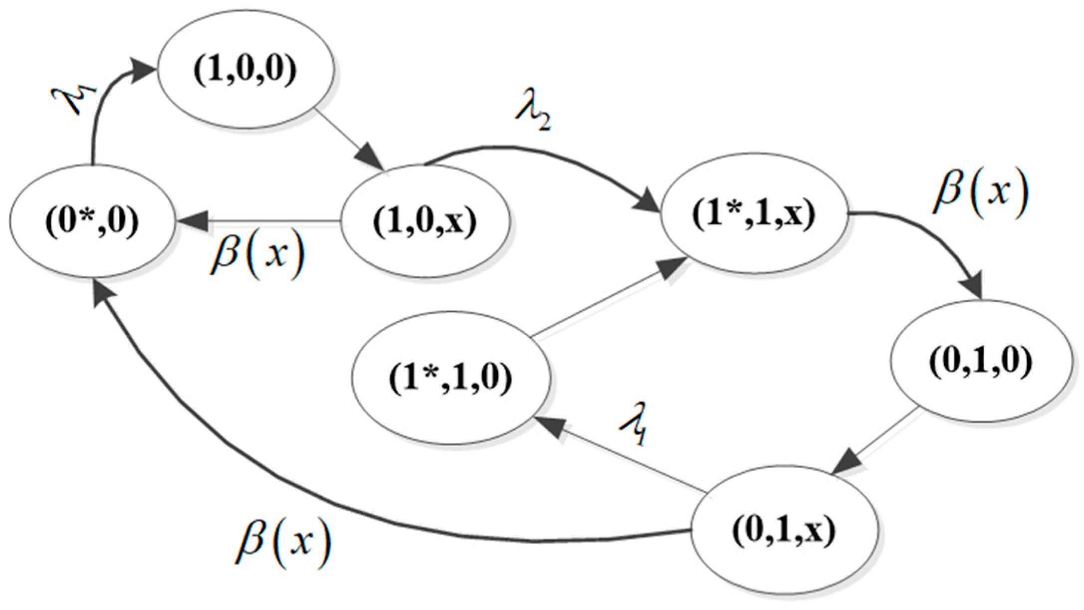
The system’s operation can be described by introducing the following set of states:
State : the main component with the priority of service is working; the second one is in cold standby.
State : the main component has failed and is under repair, the second one is working.
State : both components have failed; the main component with the priority of restoration is under repair, the second one is waiting for its turn to be repaired.
State : the main component is working; the second one is under repair.
Hereinafter, the state of the main component is marked by the asterisk symbol.
The question is to obtain the specific analytical expressions for the steady-state probabilities distribution of the system states and for the SSP of the failure-free system operation, both in the general case and for some particular distribution types. We consider a stochastic process {v(t)}, t ≥ 0, defined on the set of states where v(t) is the number of failed components of the system at time t. Using the Markov process [10] to describe the behavior of the system, we introduce a supplementary variable —the time spent by moment t to repair the failed component and use the extended set of states . Thus, we get a two-dimensional process with an expanded phase space .
We denote by , the probability that the system is in state at time t, and by , the probability density function (PDF) (over the continuous component) of the probabilities that the system is at time in state , and the time taken to repair the failed component is in the interval .
Figure 1 shows transition rate graph between states with boundary states.
We introduce two probabilities of certain auxiliary events.
First event: the component works perfectly for x units of time, before breaking within an infinitely small time interval ∆.
Second event: the failed component has been under repair for x units of time and will be repaired during time ∆, starting from the considered instant.
Theorem 1.
The steady-state probabilities of the repairable redundant system <M2/GI/1> are:
Proof of Theorem 1.
Using the total probability formula, and passing to the limit as Δ→0, we derive the Kolmogorov system of differential equations, allowing us to get the state probabilities [27] of the system in question.
With boundary conditions:
We presume that for the descriptive process, there exists a stationary probability distribution as t→∞, and we obtain a system of balance equations in the form:
With boundary conditions:
Next, we proceed to solving of this system using the constant variation method [28] and obtain the steady-state probabilities of the states of the light redundancy system. The result is the analytical expressions for the SSP of the repairable system in the following form: . Using the normalization condition we find the constant . □
4. Asymptotic Expression for the Steady-State Probabilities of the System under Rare System Failures
Let represent the Laplace transform of the repair time PDF b(x). In the case where , using the Taylor series expansion method, we obtain the following expression:
where is a k-order moment of the recovery time of a failed component and is the order number.
As an outcome, we obtain the following analytical asymptotic expressions:
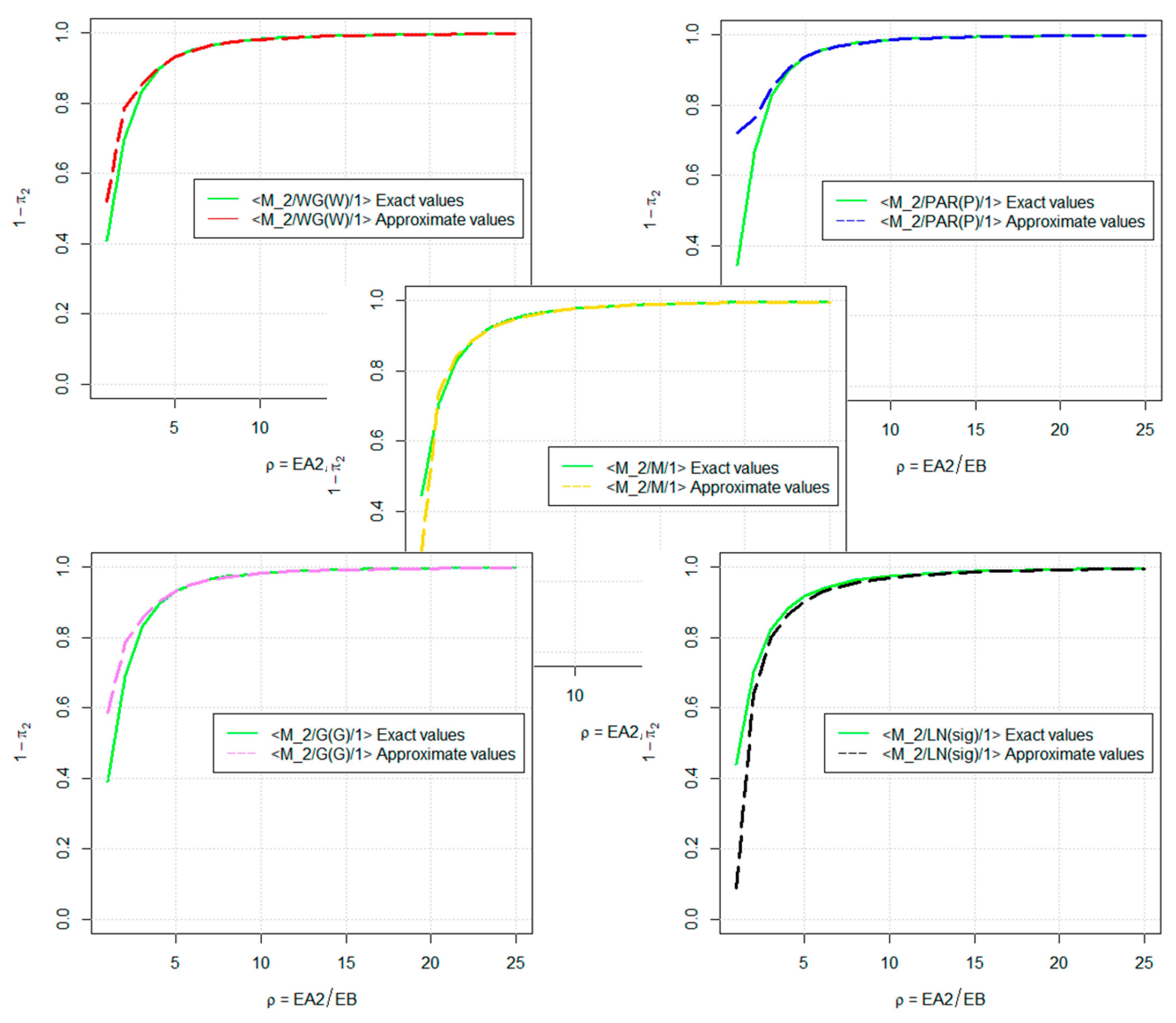
Obviously, the above expressions show that the steady-state probabilities of the system states depend on the Laplace transform of the distribution of the repair time of its components. However, with an increase in the RRR, this dependence becomes extremely low [5]. These theoretical results will be confirmed in the next section by numerical and graphical results.
5. Simulation Model for the Analysis of System-Level Reliability
5.1. Simulation Model for Assessing the System’s Steady-State Probabilities
In this subsection, we study the simulation approach, especially in the case where the considered model has arbitrary distributions of uptime and repair time of its elements.
We introduce the following variables and initial data to describe the algorithm for modeling and reliability assessment of the <GI2/GI/1> system:
double t—simulation clock; changes in case of failure or repair of the system’s elements;
int i, j—variables denoting the system’s states; when an event occurs, transition from state i to state j takes place;
double tnextfail—service variable, where time to failure of the next element is stored;
double tnextrepair—service variable, where time to next repair of the failed element is stored; and
int k—iteration counter of the main loop.
We present the simulation model in Figure 2 in the form of a block diagram. The stop criterion for the main cycle of the simulation model is hitting the maximum model run time T. The simulation pseudocode for the system <GI2/GI/1> (Algorithm A1) is given in Appendix A.
| Algorithm 1. Simulation model for assessing steady-state probabilities of the system <GI2/GI/1> |
| Initial data: A—r.v. of the failure time; B—r.v. of the recovery time; N = 2—number of system’s elements; —time to failure of elements; —moment of element’s failure in system η—time to repair of the failed element; tcur—current time; i0; i1; i2—number of failed elements; T—maximum model run time. Input: a1, a2, b1, N, T, NG, GI. a1—mean time to failure of first (main) element (FSO), a2—mean time to failure of the second element (RF), b1—mean time to repair, N—number of elements in the system, NG—number of trajectories graphs, T—maximum model run time, GI—general independent distribution function. Output: steady-state probabilities . |
5.2. Simulation Model for Assessing the System Reliability
In this subsection, we assume that if the second element of the system fails, the system fails, and the maximum model run time T equals ∞.
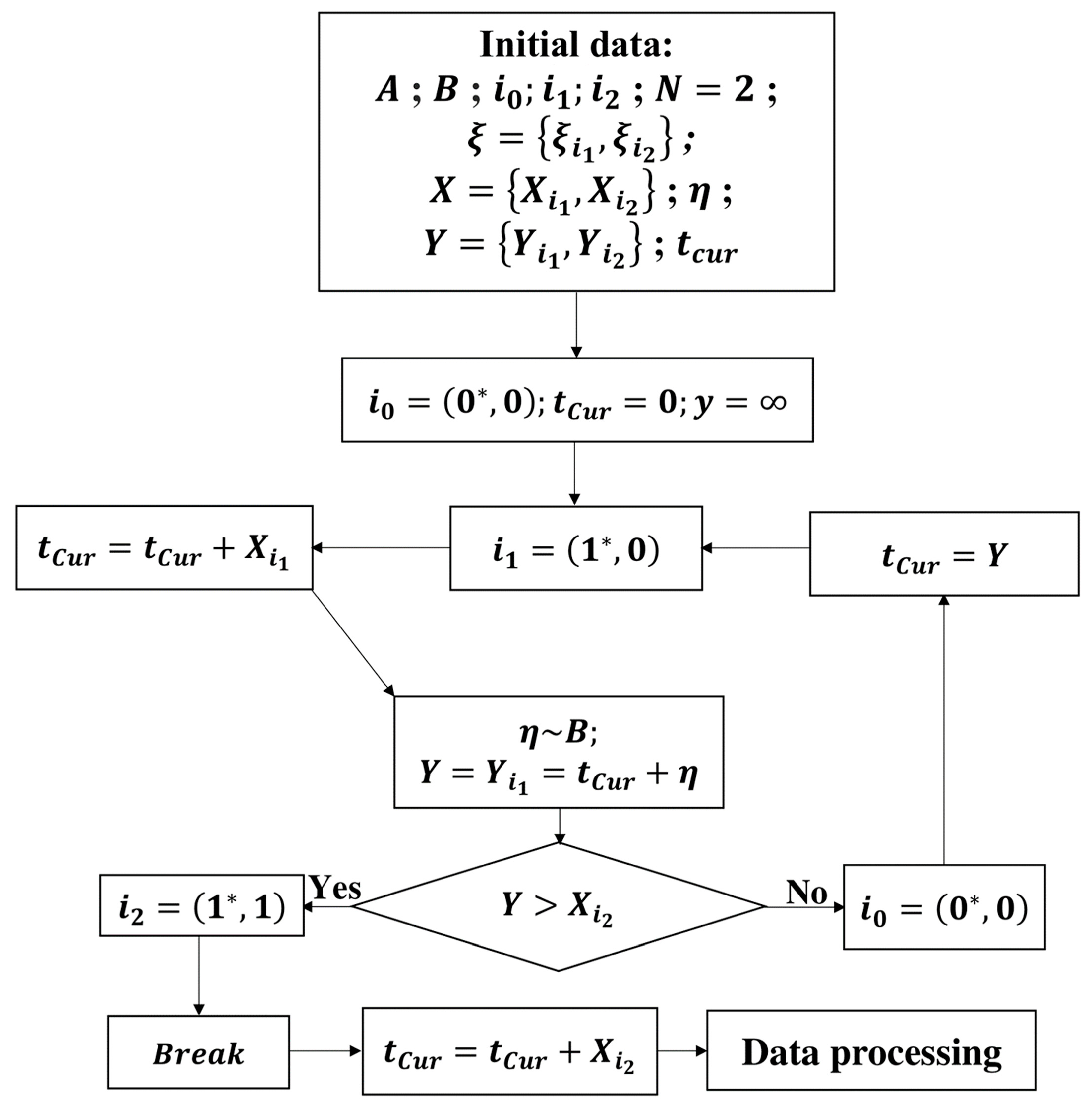
Figure 3 shows the flowchart of the simulation model for assessing system reliability. The simulation pseudocode for the system <GI2/GI/1> (Algorithm A2) is given in Appendix B.
| Algorithm 2. Simulation model for assessing the system reliability |
| Input: a1, a2, b1, N, NG, GI. Output: Assessed value of the MTTF . |
6. Numerical and Graphical Results of the Mathematical and Simulation Model
We then considered the models with the following parameter values: a1 = 25; a2 = 10; b1 = 1; N = 2; T = 100,000; NG = 1000; Lognormal (LN = 1); Gamma (G = 3); Pareto (PAR = 7); Weibull-Gnedenko (WG = 1.5); and Exponential (M).
Table 1, Table 2 and Table 3 show, respectively, the values of the steady-state probabilities, estimated values of the MTTF, and relative estimation error (Re) of the operating time until failure of the considered system, calculated by the simulation approach.
The numerical results from Table 1 show that the results obtained from simulation modeling approximate well the results obtained using analytical modeling (specific or asymptotic expression). This means that simulation modeling can be utilized in cases where it is not possible to derive formulae for the steady-state probabilities of the system states in a closed analytical form. In addition, as from Table 2, for all considered models, the models with an exponential CDF repair time of its components are reliable, especially when the system uptime has a Pareto CDF. Table 3 shows how many times the value of the estimated operating time until failure of the system </M/1> is greater than the corresponding value for </GI/1> using the formula:
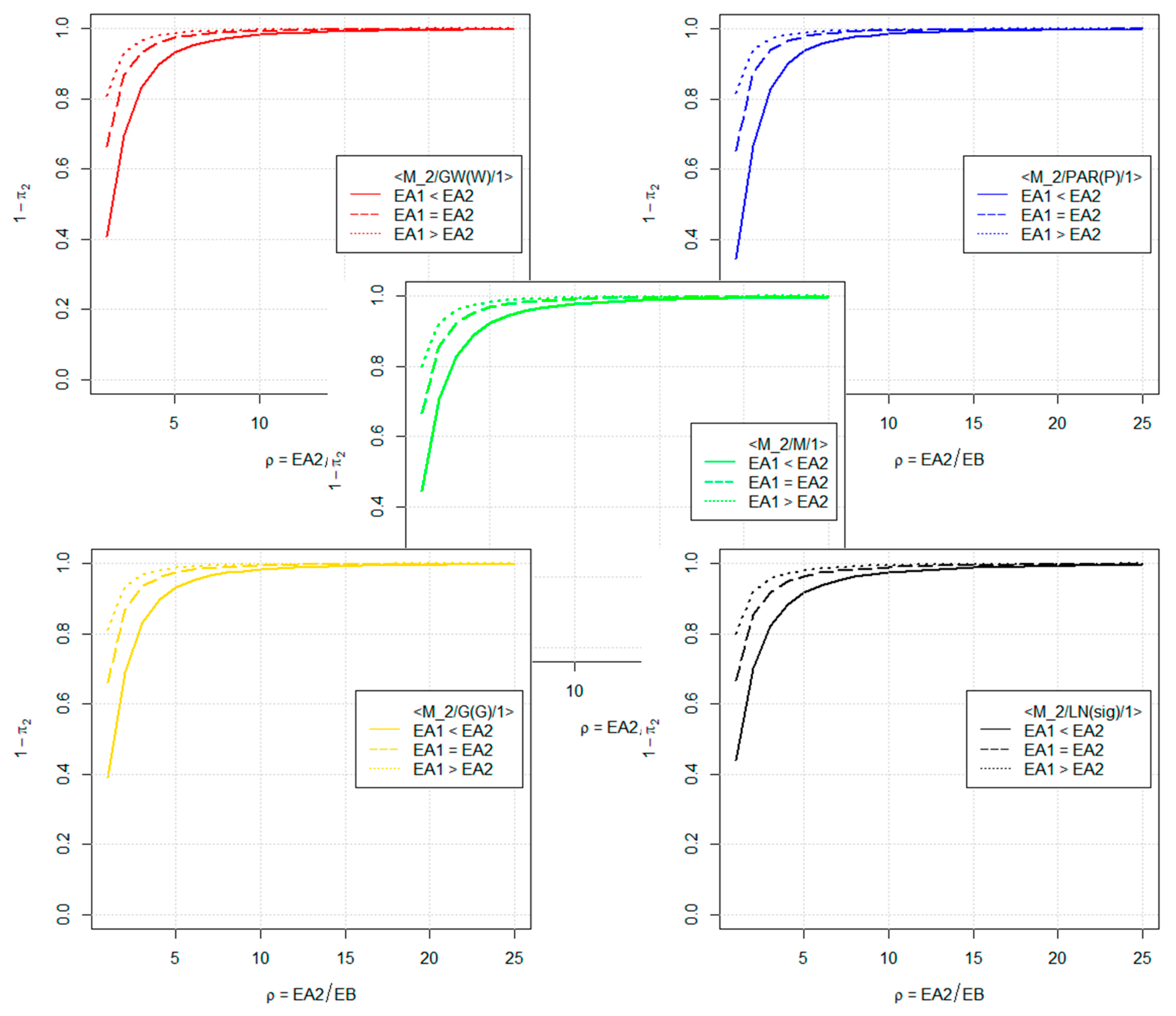
Figure 4 and Figure 5 show the graphs of the PFFO of the system from mathematical modeling. To demonstrate graphical results, we consider cases with ; where EB = 1.
Figure 6 shows the graphs of the reliability function.
The graphical results of the reliability function confirm the above conclusion about the most reliable model of all considered models.
7. Discussion
Our previous works, except for paper [23], were focused on reliability-centric analysis of homogeneous systems. Additionally, except for our paper [2], all the rest were based on studies of mathematical models. We used the same method to solve the Kolmogorov differential equations systems and get the explicit mathematical expressions for the steady-state probabilities of the system states. Of course, the results are different for each model, but the conclusion is the same. Our future research is going to be focused on mathematical modelling and simulation of a closed heterogeneous hot standby system, i.e., a special case when system components work in parallel.
8. Conclusions
We performed the analytical and asymptotic analysis for a repairable closed heterogeneous cold standby system. The exact mathematical expressions for the SSP distribution of the system states were obtained. These expressions show that the SSP of the system states depend on the Laplace transform of the components’ repair time PDF. However, with an increase in the relative rate of recovery, this dependence decreases dramatically.
The results obtained graphically from the mathematical modeling confirm the strong asymptotic insensitivity of the stationary reliability of the system under the “rapid” recovery, and prove that the longer the average uptime of the main component is, the higher the system-level reliability.
Another key finding of the research is that it is admissible to use the asymptotic expressions with increasing number of the order of the expansion in the Taylor series in those cases when it is not workable to obtain expressions for the steady-state probabilities of the system states by exact formulas.
Finally, the simulation modeling of the system has been carried out. The elaborated simulation approach allows expansion of the area of analytical research in the case of non-exponential distributions of elements’ uptime and repair time of failed elements. Numerical analysis showed that the simulation model approximates the mathematical model of the system well, and therefore can be used in cases when the system uptime distribution is general independent. Additionally, reliability function was constructed.
Author Contributions
Conceptualization, H.G.K.H. and D.K.; methodology, D.K.; software, H.G.K.H.; validation, H.G.K.H. and D.K.; formal analysis, D.K.; investigation, H.G.K.H. and D.K.; writing—original draft preparation, H.G.K.H.; writing—review and editing, D.K.; visualization, H.G.K.H.; supervision, D.K.; project administration, D.K.; funding acquisition, D.K. All authors have read and agreed to the published version of the manuscript.
Funding
This paper has been supported by the RUDN University Strategic Academic Leadership Program and funded by RFBR according to the research project No. 20-37-90137 (recipient Dmitry Kozyrev, formal analysis, validation; and recipient H.G.K. Houankpo, methodology and numerical analysis).
Institutional Review Board Statement
Not applicable.
Informed Consent Statement
Not applicable.
Acknowledgments
The authors express their gratitude to the referees for valuable suggestions that improved the quality of the paper.
Conflicts of Interest
The authors declare no conflict of interest.
Appendix A
| Algorithm A1. The simulation pseudocode for the system <GI2/GI/1> |
| Begin array r[]: = [0,0,0]; / / multi-dimensional array containing results, k-step of the main cycle double t: = 0.0; // time clock initialization int i: = 0; j: =0; // system state variables double tnextfail: = 0.0; // variable in which time until the next element failure is stored double tnextrepair: = 0.0; // variable in which time is stored until the next repair is completed int k: = 1; // counter of iterations of the main loop s[]: = rf_GI(1,λi ); // generation of an arbitrary random vector s- time to the first event (failure) sr[]: = rf_GI(1,β(x)); // generation of an arbitrary random variable sr-time of repair of the failed element) while t < ∞ do if i == 0 then s[i + 1]: = rf_GI(1,λ(i+1) ); tnextrepair: = ∞; j: = j + 1;t: = t_nextfail; end else i == 1 then else if (i − 1) == 0 then s[i + 1]: = rf_GI(1,λ(i+1)); sr[i]: = rf_GI(1,”β(x)”); tnextfail: = t + s[i + 1]; tnextrepair: = t + sr[i]; if tnextfail < tnextrepair then j: = j + 1; t: = tnextfail; else j: = j−1; t: = tnextrepair; end else if (i − 1) == N then s[i + 1]: = rf_GI(1,λ(i)); sr[i + 1]: = rf_GI(1,”β(x)”); tnextfail: = t + s[i + 1]; tnextrepair: = t + sr[i + 1]; if tnextfail < tnextrepair then j: = j + 1; t: = tnextfail; else j: = j−1; t: = tnextrepair; end end else i == N then tnextfail: = ∞; j: = j − 1; t: = tnextrepair; end if t > T then t = T end r[,,k]: = [t,i,j]; i: = j; k: = k + 1; end do Calculate estimated sojourn time in each state i, (i = 0,1,2). Stationary probabilities are calculated as: End |
Appendix B
| Algorithm A2. The simulation pseudocode for the system <GI2/GI/1> |
| Begin array r[]: = [0,0,0]; int i: = 0; int j: = 0; double tnextfail: = 0.0; double tnextrepair: = 0.0; double t: = 0.0; int k: = 1; s[]: =rf_GI(1,λi); sr: = rf_GI(1,β(x)); while t <∞ do if i == 0 then s[i + 1]: = rf_GI(1,λ(i+1)); tnextrepair: =∞; j: = j + 1;t: = t_nextfail; end else i == 1 then s[i + 1]: = rf_GI(1,λ(i+1)); sr[i]: = rf_GI(1,”β(x)”); tnextfail: = t + s[i + 1]; tnextrepair: = t + sr[i]; if tnextfail < tnextrepair then j: = j + 1; t: = tnextfail ; else j: = j − 1; t: = tnextrepair; end end else i == N thenBreak; end r[,,k]: = [t,i,j]; i: = j; k: = k + 1; end do Calculate estimated sojourn time in state N. Estimate of the MTTF of the systemis: End |
References
- Rykov, V.V.; Kozyrev, D.V. On sensitivity of steady-state probabilities of a cold redundant system to the shapes of life and repair time distributions of its elements. Springer Proc. Math. Stat. 2018, 231, 391–402. [Google Scholar] [CrossRef]
- Houankpo, H.G.K.; Kozyrev, D.V.; Nibasumba, E.; Mouale, M.N.B.; Sergeeva, I.A. A Simulation Approach to Reliability Assessment of a Redundant System with Arbitrary Input Distributions. LNCS 2020, 12563, 380–392. [Google Scholar] [CrossRef]
- Houankpo, H.G.K.; Kozyrev, D.V. Reliability Model of a Homogeneous Warm-Standby Data Transmission System with General Repair Time Distribution. LNCS 2019, 11965, 443–454. [Google Scholar] [CrossRef]
- Houankpo, H.G.K.; Kozyrev, D.V.; Nibasumba, E.; Mouale, M.N.B. Reliability Analysis of a Homogeneous Hot Standby Data Transmission System. In Proceedings of the 30th European Safety and Reliability Conference and 15th Probabilistic Safety Assessment and Management Conference (ESREL2020 PSAM15), Venice, Italy, 1–5 November 2020; pp. 1–8. [Google Scholar]
- Houankpo, H.G.K.; Kozyrev, D.V. Sensitivity Analysis of Steady State Reliability Characteristics of a Repairable Cold Standby Data Transmission System to the Shapes of Lifetime and Repair Time Distributions of Its Elements. In Proceedings of the Information and Telecommunication Technologies and Mathematical Modeling of High-Tech Systems, Moscow, Russia, 24 April 2017; Volume 1995, pp. 107–113. Available online: http://ceur-ws.org/Vol-1995/paper-15-970.pdf (accessed on 1 August 2021).
- Sijia, L.; Yuyu, W.; Zhaocai, L. Reliability analysis of general systems with bi-uncertain variables. Soft Comput. 2019, 24, 6975–6986. [Google Scholar] [CrossRef]
- Gen, Q.X.; Yan, L.L. Analysis of two components parallel repairable system with vacation. Commun. Stat.-Theory Methods 2019, 50, 2429–2450. [Google Scholar] [CrossRef]
- Xin, G.; Jiali, S.; Qingtai, W. Reliability analysis for a cold standby system under stepwise Poisson shocks. J. Control. Decis. 2021, 8, 27–40. [Google Scholar] [CrossRef]
- Liu, Y.; Qu, Z.; Li, X.; An, Y.; Yin, W. Reliability Modelling for Repairable Systems with Stochastic Lifetimes and Uncertain Repair Times. IEEE Trans. Fuzzy Syst. 2019, 27, 2396–2405. [Google Scholar] [CrossRef]
- Liu, Y.; Ma, Y.; Qu, Z.; Li, X. Reliability Mathematical Models of Repairable Systems with Uncertain Lifetimes and Repair Times. IEEE Access 2018, 6, 71285–71295. [Google Scholar] [CrossRef]
- Li, J.; Chen, Y.; Zhang, Y.; Huang, H. Availability modeling for periodically inspection system with different lifetime and repair-time distribution. Chin. J. Aeronaut. 2019, 32, 1667–1672. [Google Scholar] [CrossRef]
- Liu, B.; Qin, F.; Liu, S.; Cai, S. Reliability Modeling with Application for Calibration Data. In Proceeding of the 24th International Conference on Industrial Engineering and Engineering Management, Changsha, China, 19–20 May 2018; Springer: Singapore, 2019; pp. 133–141. [Google Scholar] [CrossRef]
- Al Turk, L.I. Characteristics and Application of the NHPP Log-Logistic Reliability Model. Int. J. Stat. Probab. 2019, 8, 44–55. [Google Scholar] [CrossRef]
- Wang, C.; Xing, L.; Peng, R. Approximate reliability analysis of large heterogeneous cold-standby systems. In Proceedings of the International Conference on Quality, Reliability, Risk, Maintenance and Safety Engineering (QR2MSE 2014), Dalian, China, 22–25 July 2014. [Google Scholar] [CrossRef]
- Abbas, B.; Javad, B.; Tore, M. Application of reliability models with covariates in spare part prediction and optimization—A case study. Reliab. Eng. Syst. Saf. 2014, 123, 1–7. [Google Scholar] [CrossRef]
- Khorshidian, K.; Fathizadeh, M. An Alternative Approach to Reliability Analysis of Cold Standby Systems. Commun. Stat.-Theory Methods 2015, 45, 6471–6480. [Google Scholar] [CrossRef]
- Parshutina, S.; Bogatyrev, V. Models to support design of highly reliable distributed computer systems with redundant processes of data transmission and handling. In Proceedings of the International Conference “Quality Management, Transport and Information Security, Information Technologies (IT&QM&IS)”, St. Petersburg, Russia, 24–30 September 2017. [Google Scholar] [CrossRef]
- The, J.; Lai, C.-M.; Cheng, Y.-H. Impact of the real-time thermal loading on the bulk electric system reliability. IEEE Trans. Reliab. 2017, 66, 1110–1119. [Google Scholar] [CrossRef]
- Lisnianski, A.; Laredo, D.; Haim, H.B. Multi-state Markov model for reliability analysis of a combined cycle gas turbine power plant. In Proceedings of the Second International Symposium on Stochastic Models in Reliability Engineering, Life Science and Operations Management (SMRLO), Beer Sheva, Israel, 15–18 February 2016. [Google Scholar] [CrossRef]
- Xu, J.J.; Xiao, Z.J. Reliability Analysis of Cold Standby Compound System. Adv. Mater. Res. 2014, 945–949, 1116–1119. [Google Scholar] [CrossRef]
- Qingtai, W. Reliability analysis of a cold standby system attacked by shocks. Appl. Math. Comput. 2012, 218, 11654–11673. [Google Scholar] [CrossRef]
- Vanderperre, E.J. Reliability analysis of a renewable multiple cold standby system. Oper. Res. Lett. 2004, 32, 288–292. [Google Scholar] [CrossRef]
- Houankpo, H.G.K.; Kozyrev, D.V.; Nibasumba, E.; Mouale, M.N.B. Mathematical Model for Reliability Analysis of a Heterogeneous Redundant Data Transmission System. In Proceedings of the 12th International Congress on Ultra-Modern Telecommunications and Control Systems and Workshops (ICUMT 2020), Brno, Czech Republic, 5–7 October 2020; pp. 189–194. [Google Scholar] [CrossRef]
- Kala, Z. Sensitivity analysis in probabilistic structural design: A comparison of selected techniques. Sustainability 2020, 12, 4788. [Google Scholar] [CrossRef]
- Letzepis, N.; Fàbregas, A. Hybrid RF/FSO communications. In Advanced Optical Wireless Communication Systems; Cambridge University Press: Cambridge, UK, 2012; pp. 273–302. [Google Scholar] [CrossRef]
- Kendall, D.G. Stochastic processes occurring in the theory of queues and their analysis by the method of embedded Markov chains. Ann. Math. Stat. 1953, 24, 338–354. [Google Scholar] [CrossRef]
- Sevastyanov, B.A. An Ergodic theorem for Markov processes and its application to telephone systems with refusals. Theor. Probab. Appl. 1957, 2, 104–112. [Google Scholar] [CrossRef]
- Petrovsky, I.G. Lectures on the Theory of Ordinary Differential Equations (Lektsii po Teorii Obyknovennykh Differentsialnykh Uravneniy); GITTL: Moscow, Russia, 1952; pp. 1–232. (In Russian) [Google Scholar]
Figure 1.
Graph of the state transition.

Figure 2.
Block diagram of the simulation model for assessing steady-state probabilities.

Figure 3.
Block diagram of the simulation model for assessing system reliability.

Figure 4.
Graphs of the probability of failure-free system operation versus .

Figure 5.
Graphs of the probability of failure-free system operation versus , constructed by exact and asymptotic formulas.
Figure 5.
Graphs of the probability of failure-free system operation versus , constructed by exact and asymptotic formulas.

Figure 6.
Graphs of the reliability function obtained by the simulation model.


Table 1.
Simulation (S), exact (E) and approximate (A) values of the steady-state probabilities of the system states with np = 2.
Table 1.
Simulation (S), exact (E) and approximate (A) values of the steady-state probabilities of the system states with np = 2.
| P0 | P1 | P2 | ||
|---|---|---|---|---|
| <M2/WG/1> | S | 0.9578 | 0.0393 | 0.0029 |
| E | 0.9579 | 0.0393 | 0.0028 | |
| A | 0.9580 | 0.0391 | 0.0029 | |
| <WG2/M/1> | S | 0.9603 | 0.0384 | 0.0014 |
| <M2/PAR/1> | S | 0.9577 | 0.0402 | 0.0021 |
| E | 0.9578 | 0.0401 | 0.0021 | |
| A | 0.9579 | 0.0400 | 0.0021 | |
| <PAR2/M/1> | S | 0.961545 | 0.038452 | 3 · 10−6 |
| <M2/G/1> | S | 0.9577 | 0.0396 | 0.0027 |
| E | 0.9579 | 0.0395 | 0.0026 | |
| A | 0.9579 | 0.0394 | 0.0027 | |
| <G2/M/1> | S | 0.9611 | 0.0385 | 0.0005 |
| <M2/LN/1> | S | 0.9579 | 0.0374 | 0.0047 |
| E | 0.9582 | 0.0374 | 0.0044 | |
| A | 0.9583 | 0.0364 | 0.0053 | |
| <LN2/M/1> | S | 0.9594 | 0.0384 | 0.0022 |
Table 2.
Estimated values of the MTTF of the system .
| <M2/WG/1> | 466.5521 |
| <WG2/M/1> | 802.1117 |
| <M2/PAR/1> | 271.7611 |
| <PAR2/M/1> | 319260.8 |
| <M2/G/1> | 280.5388 |
| <G2/M/1> | 2114.169 |
| <M2/LN/1> | 308.1753 |
| <LN2/M/1> | 483.4727 |
Table 3.
Relative estimation error (Re) of the time to failure of the system.
| GI | WG | PAR | G | LN |
|---|---|---|---|---|
| Re | 87 | 996 | 533 | 24 |
Publisher’s Note: MDPI stays neutral with regard to jurisdictional claims in published maps and institutional affiliations. |
© 2021 by the authors. Licensee MDPI, Basel, Switzerland. This article is an open access article distributed under the terms and conditions of the Creative Commons Attribution (CC BY) license (https://creativecommons.org/licenses/by/4.0/).
Share and Cite
MDPI and ACS Style
Houankpo, H.G.K.; Kozyrev, D. Mathematical and Simulation Model for Reliability Analysis of a Heterogeneous Redundant Data Transmission System. Mathematics 2021, 9, 2884. https://0-doi-org.brum.beds.ac.uk/10.3390/math9222884
AMA Style
Houankpo HGK, Kozyrev D. Mathematical and Simulation Model for Reliability Analysis of a Heterogeneous Redundant Data Transmission System. Mathematics. 2021; 9(22):2884. https://0-doi-org.brum.beds.ac.uk/10.3390/math9222884
Chicago/Turabian StyleHouankpo, Hector Gibson Kinmanhon, and Dmitry Kozyrev. 2021. "Mathematical and Simulation Model for Reliability Analysis of a Heterogeneous Redundant Data Transmission System" Mathematics 9, no. 22: 2884. https://0-doi-org.brum.beds.ac.uk/10.3390/math9222884
Note that from the first issue of 2016, this journal uses article numbers instead of page numbers. See further details here.