Monte Carlo Algorithms for the Extracting of Electrical Capacitance

Abstract

We present new Monte Carlo algorithms for extracting mutual capacitances for a system of conductors embedded in inhomogeneous isotropic dielectrics. We represent capacitances as functionals of the solution of the external Dirichlet problem for the Laplace equation. Unbiased and low-biased estimators for the capacitances are constructed on the trajectories of the Random Walk on Spheres or the Random Walk on Hemispheres. The calculation results show that the accuracy of these new algorithms does not exceed the statistical error of estimators, which is easily determined in the course of calculations. The algorithms are based on mean value formulas for harmonic functions in different domains and do not involve a transition to a difference problem. Hence, they do not need a lot of storage space.

1. Introduction

The problems of finding potentials and mutual capacitances for complex three-dimensional objects have become widespread with the development of high-frequency electrical engineering. In the case of one or two conductors, they can still be solved analytically, but solving problems for systems of a large number of conductors of complex shape causes significant difficulties. The more the operation frequency is, the more impact on the system of parasitic capacitance and induction. This is true for radio frequency communication devices, as well as very large-scale integration circuits and multilayer printed-circuit boards [1,2].

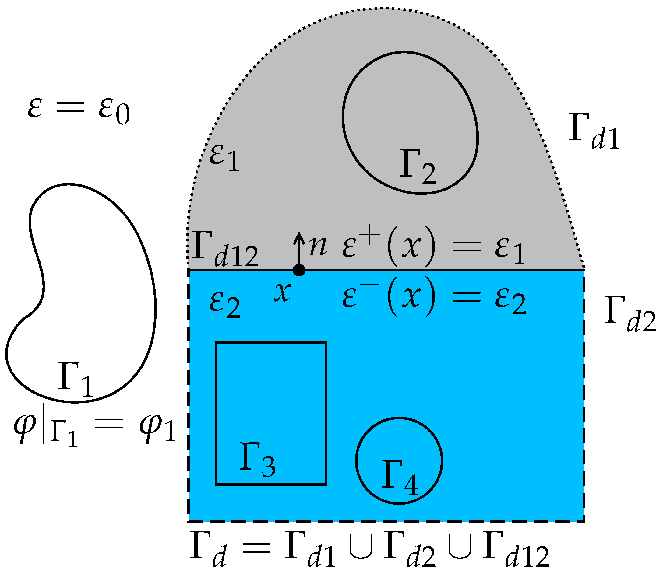
In inhomogeneous media with permittivity $\epsilon \left(x\right)$ the electrostatic potential $\phi \left(x\right)$ satisfies the boundary value problem:

$$\left.\begin{array}{c}\Delta \phi =0,x\in {\mathbf{R}}^3\backslash ({\Gamma }_i\cup {\Gamma }_d);\hfill \\ \phi \left(x\right)\underset{\left|x\right|\to \infty }{⟶}0;\hfill \\ {\phi |}_{{\Gamma }_i}={\phi }_i,{\phi }_i=\mathrm{const};\hfill \\ {\phi }^{+}\left(x\right)={\phi }^{-}\left(x\right),x\in {\Gamma }_d;\hfill \\ {\epsilon }^{+}\frac{\partial {\phi }^{+}\left(x\right)}{\partial n}={\epsilon }^{-}\frac{\partial {\phi }^{-}\left(x\right)}{\partial n},x\in {\Gamma }_d;\hfill \\ {\oint }_{{\Gamma }_i}\epsilon \frac{\partial \phi }{\partial n}dS=-q_i.\hfill \end{array}\right\}$$

(1)

Here ${\Gamma }_i$ denotes the conductor surfaces, ${\Gamma }_d$ is the union of the dielectric interfaces, n is the external normal to ${\Gamma }_d,$ $\left|x\right|$ is Euclidean length of x, ${\phi }^{+}$ and ${\phi }^{-}$ are the values of the potential on different sides dielectric interfaces, ${\epsilon }^{+}$ and ${\epsilon }^{-}$ are the permittivity constants on different sides dielectric interfaces, ${\phi }_i$ are values of the potential on the ${\Gamma }_i,$ $dS$ is the differential element of area, and $q_i$ is the charge on ${\Gamma }_i$ (Figure 1).

Charges linearly depend on potentials [3]: $q_i={\sum }_{j=1}^m{C}_{ij}{\phi }_j.$ Here, $C_{ij}$ is mutual electrostatic capacitance for the conductors i and j, it is known that $C_{ij}=C_{ji}$. Hence, $C_{ij}$ is equal to the charge $q_i,$ when all potential ${\phi }_k=0$, if $k\ne j,$ and ${\phi }_j=1.$

The analytical solution is only available for simple geometries [3], and could not be used for real-life tasks. Another way is to use pattern-matching algorithms, but there is dependency on available patterns and the quality of geometry approximation with patterns [2,4].

The methods used most for computing capacitances in complicated three-dimensional geometries are the boundary-element technique (for example, [5,6,7]) and Monte Carlo methods (for example, [8,9,10,11]).

The boundary element method is used to solve the system of integral equations of potential theory for the charge density on the surfaces of conductors. The charge on the conductor is then calculated by integrating the density. The main drawbacks of these methods are the necessity of approximation of the conductor’s surface, high random access memory requirements, and additional computational error when equations are solved using the iterative technique.

The Monte Carlo method is used to solve the Dirichlet boundary value problem (1). Capacitance is calculated using the Gaussian formula through the normal derivative of the potential. Monte Carlo algorithms for a boundary value problem are based on the representation of its solution in the form of the mathematical expectation of some random variable, which in mathematical statistics is called an unbiased estimator. A common drawback for Monte Carlo methods isthe necessity of a large number of simulations, but usually they are highly parallelizable and have low random access memory requirements.

There are various formulas for the average value for the potential, which determine both the estimate itself and the type of Random Walk along the trajectories of which it is calculated.

One of the first works on using Monte Carlo method for real-life capacitance extraction is [8]. This article describes Random Walk on Cubes methods for rectilinear conductors in a homogeneous medium. The proposed algorithm uses the mean value theorem for the potential at the center of a cube. To simplify the procedure for modeling a Random Walk, the problem was discretized. The development of the method of Random Walk on Cubes in various directions (multiple dielectrics, non-Manhattan polygonal shapes, optimizations) can be found, for example, in [12,13,14]. Besides the statistical error of Monte Carlo approximations, Walk on Cubes have additional bias because of the approximation of Green’s function for cubes using the Fourier series.

In [15], Random Walk on Boundary was described for calculating conductor’s capacitance in free space, in [9] Random Walk on Spheres and Walk on Boundary were used for estimating electrostatic properties of molecules, including cases for different (constant) permittivities. These methods were extended in [16] for analysis on multidielectric integrated circuits of arbitrary geometry from a scanning electron microscopy image. Besides the statistical error of Monte Carlo approximations, there is additional bias, because of various discretizations, that could not be estimated along with the calculations.

In this article we discuss algorithms of the Monte Carlo method that do not require discretization of the boundary value problem. Consequently, there is no approximation error in them. Due to this, it is possible to estimate the error of the approximate solution of the problem during the calculations. Furthermore, Random Walks in unbounded regions may not reach the boundary of the conductors in a finite time with a positive probability. Forced completion of the trajectory leads to a bias in the estimate of the potential, which authors usually do not take into account. Our proposed algorithms are free from this drawback.

In our previous work [10,11], we developed algorithms for mutual capacitance calculation in homogeneous media on trajectories of a Walk on Spheres and in inhomogeneous media on trajectories of a Walk on Hemispheres, when dielectric interfaces are polyhedral. We summarize the main results of these works here.

In this paper, we also consider a new version of the Walk on Hemispheres and its application to the calculation of electrostatic capacitances for systems with various dielectric interfaces, including non-Manhattan geometries.

Using the examples of conductor systems for which the capacitances are calculated analytically [3], it is shown that the accuracy of the Monte Carlo approximation is within the statistical error. In more complex examples, the simulation results are compared with the results of calculating these capacitances using the programs FastCap2 and FFTCap [6,17,18].

The paper is organized as follows. Section 2 introduces a description of the problem. Section 3 describes different kinds of unbiased estimators for the capacitance. It begins with a description of previously proposed algorithms in Section 3.1 and Section 3.2, followed by the description of a new version of the Walk on Hemispheres in Section 3.3, and finishes with a description of the generic algorithm for capacitance extraction with these methods in Section 3.4. Section 4 contains the numerical results for capacitance extraction, where we compare the results of the proposed algorithms with analytical solutions or other programs. Section 5 concludes the paper.

2. Integral Representation for the Capacitance

Using Gauss’s theorem we have

$$C_{ij}=-{\oint }_{\Gamma }\epsilon \frac{\partial \phi }{\partial n}dS,$$

(2)

where $\Gamma$ is the surface containing the i-th conductor inside and separating it from others conductors and interfaces.

Using the Poisson formula, we obtain the following representation for the normal derivative of the potential on the shell $\Gamma$:

$$\frac{\partial \phi \left(x\right)}{\partial n}=\frac{1}{4\pi r^2}{\oint }_{S_r}\frac{3}{r^2}(y-x,n)\phi \left(y\right)d_{y}S,$$

(3)

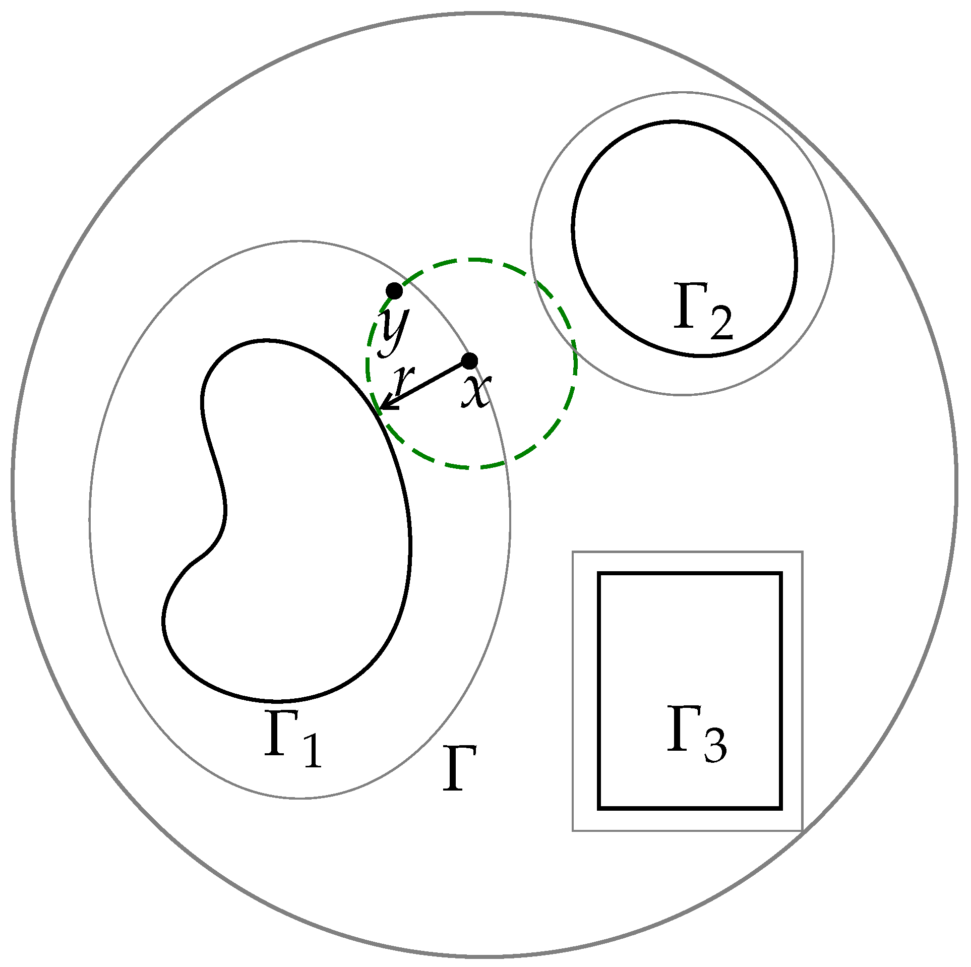
where x is a point on the shell around the i-th conductor, r is distance from point x to the nearest conductor or interface, $S_r$ is sphere of radius r centered at point x, y is a point on $S_r$ (Figure 2).

Finally, replacing the normal derivative $\partial \phi /\partial n$ by its integral representation in the ball, which lies entirely in the region with the dielectric constant $\epsilon$, we obtain an integral representation of the mutual capacitance of the i-th and j-th conductors:

$$C_{ij}=-\frac{1}{{\sigma }_{\Gamma }}{\oint }_{\Gamma }\frac{\epsilon }{r^2}{\oint }_{S_r}\frac{3{\sigma }_{\Gamma }}{4\pi r^2}(y-x,n)\phi \left(y\right)d_{y}S{d}_{x}S,$$

(4)

where ${\sigma }_{\Gamma }$ is a surface area $\Gamma$.

3. Unbiased Estimators for the Capacitance

Using Formula (4) we have unbiased estimator for capacitance $C_{ij}$

$$\xi =\frac{3\epsilon \left(X\right){\sigma }_{\Gamma }}{r}(\omega ,n)\phi (X+r\omega ).$$

(5)

Here, a random point X is uniformly distributed on $\Gamma ,$$r=r\left(X\right),$ and $\omega$ is an isotropic vector (random unit vector). It remains to estimate the potential at the point $Y=X+r\left(X\right)\omega .$ This can be done using the mean value formula

$$\phi \left(x\right)={\int }_Q\phi \left(y\right)P(x,dy),x\in Q,$$

(6)

where $Q={\mathbf{R}}^3\backslash D,$ and D is the set of interior points of all conductors. The unbiased estimators for $\phi \left(Y\right)$ are constructed on trajectories of Random Walk ${\left\{Y_k\right\}}_{k=0}^{\infty }$, $(Y_0=Y)$, in space Q. The kernel $P(x,dy)$ must be stochastic or sub-stochastic. It determines the distribution of the next point of the Random Walk over the current point.

Let

$${\xi }_0=\frac{3\epsilon \left(X\right){\sigma }_{\Gamma }}{r}(\omega ,n).$$

(7)

If at time k the “weight” $W_k=P(Y_k,Q)<1$, then the current value of the estimator is multiplied by the “weight”: ${\xi }_{k+1}=W_k{\xi }_k.$ The Random Walk stops at time $\nu$, when it reaches the $\delta$-boundary of the conductors, that is, when the distance $\mathrm{dist}(Y_k,\partial \overline{D})$ from point $Y_k$ to the boundary of the conductors becomes less than the $\delta .$ Hence, it must satisfy the condition $P\{\nu <\infty \}=1.$ We define estimator ${\xi }_{\delta }={\xi }_{\nu },$ if $\mathrm{dist}(Y_{\nu },{\Gamma }_j)<\delta$, and zero, otherwise. If the boundary $\partial D$ is smooth enough, then $|C_{ij}-E{\xi }_{\delta }|<c\delta ,$ for some constant $c.$ In practice, the estimator ${\xi }_{\delta }$ is simulated in a reasonable time, only if $E{\xi }_{\nu }<\infty .$ Having received a sufficient number of realizations of the estimator ${\xi }_{\delta }$ and calculating their arithmetic mean, we obtain an approximate value of the capacitance $C_{ij}.$

We will now describe some of the types of Random Walks used to calculate the capacitances of conductors.

3.1. Random Walk on Spheres for the External Dirichlet Problem

Random Walk on Spheres (WoS) is used to solve the external Dirichlet problem for the Laplace equation [19], and allows for the calculation of the capacitances of conductors in a homogeneous medium [10]. Let all the conductors lie inside a sphere $S_R$ of radius R centered at the origin. Let $\rho \left(y\right)$ be a continuous function such that $c·\mathrm{dist}(y,\partial \overline{D})\le \rho \left(y\right)\le \mathrm{dist}(y,\partial \overline{D})$ for some constant $c>0.$

By the mean value theorem for harmonic functions, we obtain $\phi \left(x\right)=E\phi \left(x+\rho \left(x\right)\omega \right)$ for $x\in {\mathbf{R}}^3\backslash \overline{D}.$ Let ${\left\{{\omega }_k\right\}}_{k=1}^{\infty }$ be a sequence of independent isotropic vectors. Then we get a Random Walk

$$\begin{array}{cc}\hfill Y_{k+1}& =Y_k+\rho \left(Y_k\right){\omega }_{k+1},\hfill \\ \hfill Y_0& =Y,\hfill \\ \hfill W_k& =1,\hfill \\ \hfill k& =0,1,2,\dots .\hfill \end{array}$$

To restrict the region of the Random Walk, we use the Poisson formula for $\left|x\right|>R$:

$$\phi \left(x\right)=\frac{1}{4\pi R}{\oint }_{S_R}\frac{{\left|x\right|}^2-R^2}{{|x-y|}^3}{d}_{y}S.$$

Namely, if $|Y_k|>R$, then “weight” $W_k=R/\left|Y_k\right|,$ and $Y_{k+1}$ is distributed on the sphere $S_R$ with density

$$p(Y_k,y)=\frac{|Y_k{|}^2-R^2}{|Y_k{-y|}^3}·\frac{|Y_k|}{4\pi R^2}$$

(8)

(Figure 3).

It is proved [19] that the Random Walk on Spheres reaches the $\delta$-neighborhood of the boundary of the conductors in a finite time. The formulas for simulating the Random Walk are also given.

3.2. Random Walk on Hemispheres

The Random Walk on Hemispheres (WoH) algorithm was proposed in [20] for solving various boundary value problems for the Laplace and Poisson equations. It allows for the calculation of capacitances when dielectric interfaces are polyhedral [11]. In cases when surfaces of the conductors are also polyhedral, the algorithm gives unbiased statistical estimators of the capacitances. We will now briefly describe this algorithm.

Let all the conductors and dielectric interfaces lie inside a sphere $S_R$ of radius R centered at the origin. If $|Y_k|>R$, then $Y_{k+1}\in S_R$ and has a distribution density (8). “Weight” $W_k=R/\left|Y_k\right|.$

Now, let $Y_k\in {\Gamma }_{d_l}$, where ${\Gamma }_{d_l}$ is a component of the dielectric interface. Next, we choose the maximum $r,$ such, that $0<r<\mathrm{dist}(Y_k,\overline{D}\cup {\Gamma }_d\backslash {\Gamma }_{d_l})$ and part of the ${\Gamma }_{d_l},$ lying in sphere $S_r\left(Y_k\right),$ is plane. The sphere is divided into two parts $S_r^{+}\left(Y_k\right)$ and $S_r^{-}\left(Y_k\right)$ lying in media with permittivity constants ${\epsilon }^{+}$ and ${\epsilon }^{-}$, respectively. The point $Y_{k+1}$ is uniformly distributed in $S_r^{+}\left(Y_k\right)$ or in $S_r^{-}\left(Y_k\right)$ with probability ${\epsilon }^{+}/({\epsilon }^{+}+{\epsilon }^{-})$ and ${\epsilon }^{-}/({\epsilon }^{+}+{\epsilon }^{-})$ respectively (Figure 4).

If $Y_k\notin {\Gamma }_d$ and $|Y_k|\le R$, then $Y_{k+1}$ is distributed on a sphere or hemisphere. The center of the hemisphere ${\widehat{Y}}_k$ must be in a plane containing a face of the conductor surface or interface and is the orthogonal projection of $Y_k$ onto this plane.

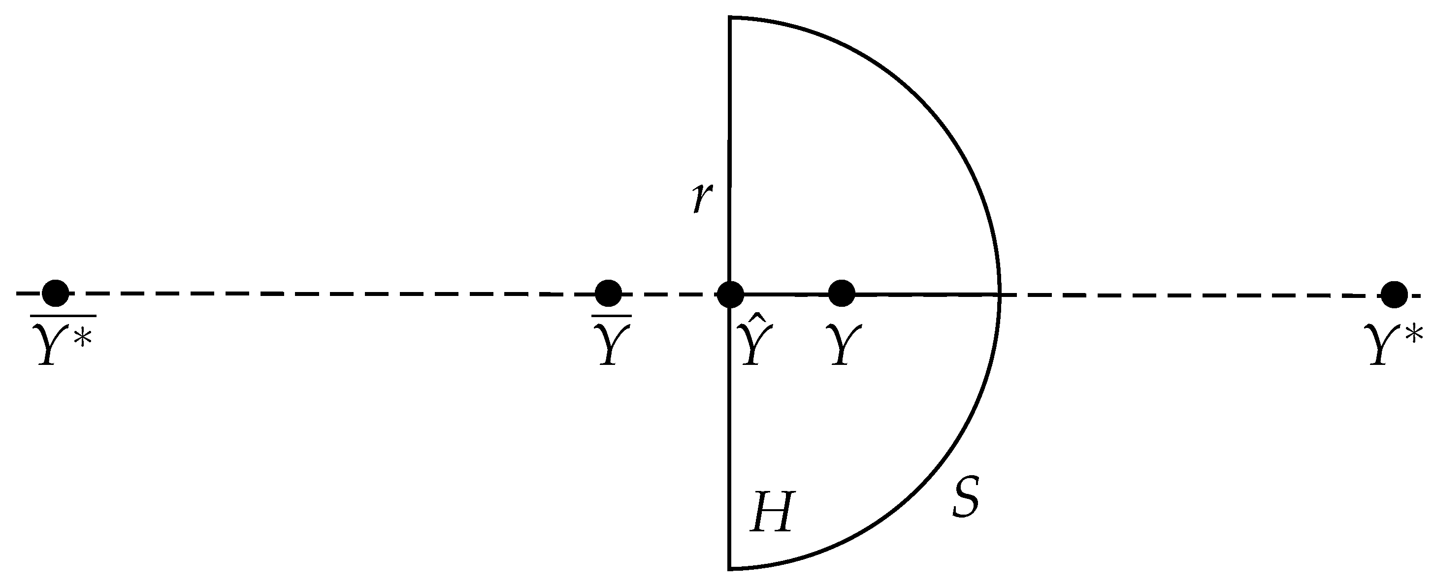
Hemisphere radius $r_k=|Y_k-{\widehat{Y}}_k|/\beta$, where $0<\beta <1$ is a fixed constant. The hemisphere must be contained in a medium with a dielectric constant $\epsilon \left(Y_k\right)$. The distribution density of the point $Y_{k+1}$ on the hemisphere is the normal derivative of the Green’s function for the half of the ball

$$p(Y_k,y)=\left\{\begin{array}{cc}\frac{2r_k\beta }{4\pi }\left(\frac{1}{|Y_k{-y|}^3}-\frac{1}{{\left(\beta |\overline{Y_k^{*}}-y|\right)}^3}\right),\hfill & y\in H,\hfill \\ \frac{r_k}{4\pi }\left(1-{\beta }^2\right)\left(\frac{1}{|Y_k{-y|}^3}-\frac{1}{|\overline{Y_k}{-y|}^3}\right),\hfill & y\in S.\hfill \end{array}\right.$$

(9)

Here H is the plane part, and S is the spherical part of the hemisphere. The point $\overline{Y_k}$ is symmetric to $Y_k$ relative to plane H. The point $Y_k^{*}$ lies outside of the sphere S and it is inverse to the point $Y_k$ ($|{\widehat{Y}}_k-Y_k|·|{\widehat{Y}}_k-Y_k^{*}|=r^2$) (Figure 5).

If it is impossible to construct such a hemisphere, then $Y_{k+1}$ is distributed uniformly on a sphere of radius $r_k=\mathrm{dist}(Y_k,\overline{D}\cup {\Gamma }_d)$, centered at $Y_k$.

Von Neumann’s Acceptance-Rejection Method can be used to simulate density (9). To do this, we write the density in the form

$$p(Y_k,y)=\frac{1}{4\pi }\frac{cos{\phi }_{Y_{k}y}}{{\left|Y_k-y\right|}^2}·k_1(Y_k,y),$$

(10)

where ${\phi }_{Y_{k}y}$ is the angle between the vector $y-Y_k$ and the external normal to the surface of the hemisphere at the point y.

The first factor in this formula is the distribution density of the point Z on the surface of the hemisphere and the vector $\omega =(Z-Y_k)/|Z-Y_k|$ is isotropic one. The second factor does not exceed the constant $M=max(M_1,M_2)$, where

$$\begin{array}{cc}\hfill M_1& =\frac{2}{\beta }\sqrt{1+{\beta }^2}\left(1-{\left(\frac{\beta }{\sqrt{1+{\beta }^2}}\right)}^3\right),\hfill \\ \hfill M_2& =\sqrt{1+{\beta }^2}\frac{1+\beta }{1-\beta }\left(1-{\left(\frac{1-\beta }{1+\beta }\right)}^3\right).\hfill \end{array}$$

To select the next point of the random walk, we simulate an isotropic vector $\omega$ and a random variable $\alpha$ with uniform distribution on $[0,1]$. Then we define the point Z, in which the ray emerging from the $Y_k$ in the direction $\omega$ crosses the hemisphere. If $\alpha M<k_1(Y_k,Z)$, then $Y_{k+1}=Z$. Otherwise, it is necessary to repeat the simulation until the inequality is true (Figure 6).

3.3. Random Walk on Hemispheres for a Convex Dielectric Interfaces (RWHC)

Let $\gamma$ be a connected convex part of some dielectric interface ${\Gamma }_{d_l}$ lying inside a sphere $S_r\left(x\right)$ of radius $r,$ centered at point $x.$ For all $y\in {\Gamma }_{d_l}$ we choose the direction of the normal vector $n_y$ so, that the surface ${\Gamma }_{d_l}$ lies in the half-space $(z-y,n_y)\le 0$. Surface $\gamma$ divides the sphere into two parts $S^{+}$ and $S^{-},$ lying in media with permittivity constants ${\epsilon }^{+}$ and ${\epsilon }^{-}$, respectively, and $(z-y,n_y)\le 0$ for all $z\in S^{-}.$

The potential $\phi \left(x\right)$ is a harmonic function for the part of the ball bounded by surfaces $S^{-},$$\gamma$ and part of the ball bounded by surfaces $S^{+},$$\gamma$ also. Using the second Green’s formula for a harmonic function in a bounded domain, we obtain the following Theorem.

Theorem 1.

Let $\lambda ={\epsilon }^{+}/{\epsilon }^{-}$ and let ${\phi }_{xy}$ be the angle between vectors $n_y,$$y-x.$ Then the potential $\phi \left(y\right)$ satisfies the mean value formulas:

$$\begin{array}{c}\phi \left(x\right)=\frac{1}{1+\lambda }·\frac{1}{2\pi r^2}{\int }_{S^{-}}\phi \left(y\right)d_{y}S+\frac{\lambda }{1+\lambda }·\frac{1}{2\pi r^2}{\int }_{S^{+}}\phi \left(y\right)d_{y}S+\hfill \\ \hfill +\frac{1-\lambda }{1+\lambda }·\frac{1}{2\pi }{\int }_{\gamma }\frac{cos{\phi }_{xy}}{{|x-y|}^2}\phi \left(y\right)d_{y}S,x\in \gamma ,\end{array}$$

(11)

$$\begin{array}{c}\phi \left(x\right)=\frac{1}{4\pi r^2}{\int }_{S^{-}}\phi \left(y\right)d_{y}S+\lambda ·\frac{1}{4\pi r^2}{\int }_{S^{+}}\phi \left(y\right)d_{y}S+\hfill \\ \hfill +(1-\lambda )·\frac{1}{4\pi }{\int }_{\gamma }\frac{cos{\phi }_{xy}}{{|x-y|}^2}\phi \left(y\right)d_{y}S,x\notin \gamma ,\epsilon \left(x\right)={\epsilon }^{-},\end{array}$$

(12)

$$\begin{array}{c}\phi \left(x\right)=\frac{1}{4\pi r^2}{\int }_{S^{+}}\phi \left(y\right)d_{y}S+\frac{1}{\lambda }·\frac{1}{4\pi r^2}{\int }_{S^{-}}\phi \left(y\right)d_{y}S-\hfill \\ \hfill -\left(1-\frac{1}{\lambda }\right)·\frac{1}{4\pi }{\int }_{\gamma }\frac{cos{\phi }_{xy}}{{|x-y|}^2}\phi \left(y\right)d_{y}S,x\notin \gamma ,\epsilon \left(x\right)={\epsilon }^{+}.\end{array}$$

(13)

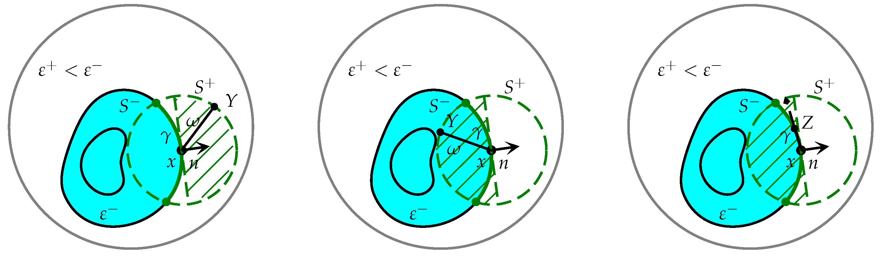
If $\lambda <1,$ the Formula (11) defines the stochastic kernel. To simulate the transition from the surface $\gamma$, we chose with the probability $\lambda /(1+\lambda )$ a random direction $\omega ,$ that satisfies the condition $(\omega ,n_x)>0,$ and define $Y=x+r\omega .$ With probability $1/(1+\lambda ),$ we simulate a random direction $\omega$ satisfying the condition $(\omega ,n_x)<0.$ We calculate $Y=x+r\omega .$ If $Y\notin S^{-}$, we change Y to a point $Z\in \gamma$, which is visible from x in the direction $\omega$ (Figure 7).

If $\lambda <1,$ the Formula (12) defines the stochastic kernel also. To simulate the transition from $x,$ we simulate a random direction $\omega$ and calculate $Y=x+r\omega .$ If $Y\notin S^{-}$, than with probability $1-\lambda$ we change Y to a point $Z\in \gamma$, which is visible from x in the direction $\omega$ (Figure 8).

If $\lambda >1,$ the Formula (13) defines the stochastic kernel, if any ray outgoing from point x intersects $\gamma$ at no more than one point. The modeling procedure is similar to the algorithm for the Formula (12).

Thus, Formulas (11)–(13) make it possible to simulate transitions from a region with a higher dielectric constant to a region with a lower dielectric constant. To pass from point x through the interface ${\Gamma }_{d_l}$, it is sufficient to take such $r\le \mathrm{dist}(x,\overline{D}\cup {\Gamma }_d\backslash {\Gamma }_{d_l})$ that $S_r\left(x\right)\cap {\Gamma }_{d_l}\ne \varnothing .$ Reverse transitions can be provided using, for example, formulas for solving external and internal Dirichlet problems for standard domains. The exit from the “bad” point x can be done by Random Walk on Spheres or Hemispheres in the set $Q\left(x\right)=\left\{y\right|\epsilon \left(y\right)=\epsilon \left(x\right)\}.$ As always, from distant points of the external medium there is a transition to the sphere $S_R.$

3.4. Algorithm for Mutual Capacitance Calculation

On this basis we could describe algorithm for capacitance estimation as follows:

• For each conductor i select shell ${\Gamma }_i$, that separate it from other conductors and dielectric interfaces.
• Select radius R for, centered at the origin, “outer” sphere, that contains all conductors and shells.
• Select point X uniformly on ${\Gamma }_i$ and Y uniformly on sphere of radius $r=r\left(X\right)=\mathrm{dist}(X,{\cup }_{k=1,k\ne i}^n{\Gamma }_k)$ centered at X. Set ${\xi }_0$ as shown in (7).
• From point Y started appropriate kind of Walk on Hemispheres (see Section 3.2 and Section 3.3).
• If at some step n process exit outside of sphere $S_R$, next point is selected at sphere $S_R$ and “weight” updated, as described in Section 3.1.
• Otherwise, if at some step n, $Y_n$ located at flat surface of k-th conductor or at $\delta$-neighborhood of non-flat surface of k-th conductor, estimation ${\xi }_n$ included into $C_{ik}$ accumulator and number of trajectories, that used this conductor for evaluation is incremented by 1. (Because $C_{ij}=C_{ji}$, we could use the same accumulator and counter for both of them.) Values in other accumulators $C_{ij}$ are not changed, but the number of trajectories for j-th conductor is also incremented by 1 with the exception of nested conductors: if j-th conductor is inside i-th, its number of trajectories is not changed.
• If the number of evaluated trajectories is not sufficient, return to step 3.
• The approximation for capacitance $C_{ik}$ is calculated as value stored in the corresponded accumulator divided by the stored number of trajectories for this accumulator. If the system contains nested conductors, the self-capacitance of external conductor m is updated as $C_{mm}=C_{mm}-{\sum }_{j:D_j\subset D_m}{C}_{jm}$ (here sum is taken by numbers of conductors that are located inside m-th).

4. Results

4.1. Mutual Capacitance of Two Spheres in Free Space

Mutual capacitance for two spheres could be calculated analytically [3]. When spheres are not nested:

$$\begin{array}{cc}\hfill C_{1,1}& =4\pi \epsilon r_1{r}_{2}sinh\alpha \sum _{n=1}^{\infty }{\displaystyle \frac{1}{r_{2}sinh\left(n\alpha \right)+r_{1}sinh\left[(n-1)\alpha \right]}};\hfill \\ \hfill C_{1,2}& =-4\pi \epsilon {\displaystyle \frac{r_1{r}_{2}sinh\alpha }{d}}\sum _{n=1}^{\infty }{\displaystyle \frac{1}{sinh\left(n\alpha \right)}};\hfill \\ \hfill C_{2,2}& =4\pi \epsilon r_1{r}_{2}sinh\alpha \sum _{n=1}^{\infty }{\displaystyle \frac{1}{r_{1}sinh\left(n\alpha \right)+r_{2}sinh\left[(n-1)\alpha \right]}};\hfill \\ \hfill cosh\alpha & ={\displaystyle \frac{d^2-r_1^2-r_2^2}{2r_1{r}_2}}\hfill \end{array}$$

where $r_1$ and $r_2$ are radii, d—distance between sphere centers. For nested spheres ($r_2>r_1$):

$$\begin{array}{cc}\hfill C_{1,1}& =4\pi \epsilon r_1{r}_{2}sinh\alpha \sum _{n=1}^{\infty }{\displaystyle \frac{1}{r_{2}sinh\left(n\alpha \right)-r_{1}sinh\left[(n-1)\alpha \right]}};\hfill \\ \hfill C_{1,2}& =-C_{1,1};\hfill \\ \hfill cosh\alpha & =-{\displaystyle \frac{d^2-r_1^2-r_2^2}{2r_1{r}_2}}.\hfill \end{array}$$

In

Table 1. Mutual capacitance estimation for two non-nested spheres, $C_{i,j}/4\pi {\epsilon }_0$.

Method	$1,1$	$\mathbf{\Delta }$	$1,2$	$\mathbf{\Delta }$	$2,2$	$\mathbf{\Delta }$	Time	Memory
Analytical	$5.29133$	–	$-0.94883$	–	$3.18564$	–	–	–
WoS, ${10}^5$	$5.14975$	$2.711·{10}^{-1}$	$-0.93335$	$5.799·{10}^{-2}$	$3.24719$	$1.268·{10}^{-1}$	–	11 Mb
WoS, ${10}^7$	$5.2965$5	$2.717·{10}^{-2}$	$-0.94894$	$5.805·{10}^{-3}$	$3.19233$	$1.263·{10}^{-2}$	40 s	11 Mb

results of mutual capacitance estimation for two non-nested spheres using Walk on Spheres are presented. Here and below $\Delta$ is error estimation, calculated as triple square root of ratio of sample variance to number of trajectories, Time is “wall time” of calculation, and Memory is a peak memory usage. Calculations were performed on one personal computer (PC) with central processing unit (CPU) “AMD Ryzen 7 2700 Eight-Core Processor 3.20 GHz”. Monte Carlo simulations were performed in parallel by eight worker processes on one PC using the Message Passing Interface, and memory usage is at its peak for one worker process. FastCap2 and FFTCap are 32-bit single-threaded applications, so no parallel execution were used for them. It should also be noted that we have not used additional optimizations, so the calculation time could be improved for the Monte Carlo case, for example, by using a different pseudo random number generator or using optimizations in distance calculations.

1st sphere radius:	5;
1st sphere center:	(1, 2, 3);
1st sphere shell radius:	8;
2nd sphere radius:	3;
2nd sphere center:	(10, 13, 12);
2nd sphere shell radius:	8;
“External” sphere radius:	31.155;
$\delta$: ${10}^{-8}$.

Usually, the bias order is the same as the order of $\delta$, so, in this and following examples, error of methods is equal to statistical error. We will say that results of the estimation are matched, when the modulus of difference between the Monte Carlo estimation and the reference solution are not more than the statistical error ($|ref-est|\le \Delta$). As we can see in the Table 1, the analytical solution and our estimation are matched, so the algorithm is working correctly.

In

Table 2. Mutual capacitance estimation for two nested spheres, $C_{i,j}/4\pi {\epsilon }_0$.

Method	1,1	$\mathbf{\Delta }$	1,2	$\mathbf{\Delta }$	Time	Memory
Analytical	$3.47735$	–	$-3.47735$	–	–	–
WoS, ${10}^5$	$3.48643$	$1.531·{10}^{-1}$	$-3.53438$	$1.292·{10}^{-1}$	–	11 Mb
WoS, ${10}^7$	$3.47455$	$1.531·{10}^{-2}$	$-3.47807$	$1.289·{10}^{-2}$	30 s	11 Mb

, results of mutual capacitance estimation for two nested spheres using Walk on Spheres (WoS) are presented. There is no formula for $C_{22}$ in the case of two nested spheres in [3], so we do not show the estimation results for this value.

1st sphere radius:	3;
1st sphere center:	(10, 13, 12);
1st sphere shell radius:	5;
2nd sphere radius:	31;
2nd sphere center:	(1, 2, 3);
2nd sphere shell radius:	35;
“External” sphere radius:	42.616;
$\delta$: ${10}^{-8}$.

Estimation results in Table 2 are within statistical error, so analytical solution and our estimation are matched.

4.2. Capacitance of “Coated” Sphere

In

Table 3. Capacitance estimation for coated sphere, $C/4\pi {\epsilon }_0$.

$\mathit{a}=1$, $\mathit{b}=3$	Anal.	FC2	RWHC, ${10}^6$	$\mathbf{\Delta }$	RWHC, ${10}^8$	$\mathbf{\Delta }$
$\epsilon =2$	$1.5000$	$1.5018$	$1.4813$	$3.111·{10}^{-2}$	$1.4994$	$3.114·{10}^{-3}$
$\epsilon =10$	$2.5000$	$2.5872$	$2.4403$	$1.889·{10}^{-1}$	$2.5094$	$1.889·{10}^{-2}$
$\epsilon =100$	$2.9411$	$4.3926$	$2.7198$	$2.055$	$2.8966$	$2.055·{10}^{-1}$

and

Table 4. Capacitance estimation for coated sphere. Time and memory usage.

	FC2	RWHC, ${10}^8$
$a=1$, $b=3$, $\epsilon =2$
Time, s	9	158
Memory, Mb	899	11
$a=1$, $b=3$, $\epsilon =10$
Time, s	9	148
Memory, Mb	899	11
$a=1$, $b=3$, $\epsilon =100$
Time, s	9	147
Memory, Mb	900	11

, results of capacitance estimation for the conductive sphere of radius a encased in concentric spherical dielectric of radius b with relative permittivity $\epsilon$ using RWHC are presented. In this example, the external sphere radius is equal to the dielectric shell radius. Analytical solutions for this case is ${\displaystyle \frac{16{\pi }^2\epsilon {\epsilon }_{0}ab}{\epsilon a+b-a}}$ [3]. Also here we compare results with FastCap2 (FC2) [18] (correspondent sphere discretization was made using spheregen tool from [21] with refine depth 5).

Comparing values in columns 2, 4, 5 of Table 3 we conclude that the analytical solution and RWHC estimation are matched in all cases. However, comparing columns 2 and 3, we can see that the estimation error for FC2 grows up with $\epsilon$ (as it is stated in [7]). So we can state, that RWHC working correctly with high permittivities too, but more number of simulation may be needed to get estimation with desired statistical error.

Table 4 shows that RWHC is used more often than boundary-element technique-based methods, such as FC2, but use much less memory.

4.3. Mutual Capacitance of Two Spheres in Spherical Dielectric

In the

Table 5. Mutual capacitance estimation for two spheres in dielectric shell, $C_{i,j}/4\pi {\epsilon }_0$.

$\mathit{i},\mathit{j}$	FC2	RWHC, ${10}^6$	$\mathbf{\Delta }$	RWHC, ${10}^8$	$\mathbf{\Delta }$
$\epsilon =2$
$1,1$	$9.8444$	$9.9718$	$1.597·{10}^{-1}$	$9.8192$	$1.598·{10}^{-2}$
$1,2$	$-3.3396$	$-3.3463$	$2.254·{10}^{-2}$	$-3.3440$	$2.260·{10}^{-3}$
$2,2$	$6.0965$	$6.1454$	$6.760·{10}^{-2}$	$6.0968$	$6.755·{10}^{-3}$
$\epsilon =10$
$1,1$	$33.262$	$33.440$	$8.264·{10}^{-1}$	$32.890$	$8.270·{10}^{-2}$
$1,2$	$-21.038$	$-21.045$	$1.317·{10}^{-1}$	$-21.118$	$1.318·{10}^{-2}$
$2,2$	$25.380$	$25.424$	$3.495·{10}^{-1}$	$25.276$	$3.494·{10}^{-2}$

and

Table 6. Mutual capacitance estimation for two spheres in dielectric shell. Time and memory usage.

	FC2	RWHC, ${10}^8$
$\epsilon =2$
Time, min	13	3
Memory, Mb	1710	11
$\epsilon =10$
Time, min	14	3
Memory, Mb	1712	11

results of mutual capacitance estimation using FC2 (correspondent sphere discretization was made using spheregen tool from [21] with refined depth 5) and RWHC for two conductive spheres in spherical dielectric (Figure 9) are presented. In this case external sphere radius is set to the dielectric shell radius.

1st sphere radius:	5;
1st sphere center:	(1, 2, 3);
1st sphere shell radius:	6;
2nd sphere radius:	3;
2nd sphere center:	(10, 3, 11);
2nd sphere shell radius:	4;
Dielectric ball radius:	20;
$\delta$: ${10}^{-8}$.

In this case we have no analytical solutions for reference, so we compare our results with FC2. But we also have no error estimation for FC2 result, so we could not guarantee that the difference will be within statistical margin of error. Comparing results in columns 2 and 3 of Table 5 we could say that the estimations are matched, but it is not true for columns 2 and 4. In previous cases we ascertained that RWHC is matched with the analytical solution. Also, in this case, we can see that results in columns 3 and 4 are matched. So we can state that in this case the estimation error with FC2 is more than with RWHC on ${10}^8$ trajectories.

In Table 6 we can see that RWHC is better both in time and memory. This is due to the fact that for FC2 spheres should be approximated with a large number of panels. Also, we can see that with the refinement depth we used, we have almost reached the memory limit for the original 32-bit fastcap application, so we cannot compare to these results with better discretization.

4.4. Mutual Capacitance of Two Spheres in Spherical Dielectrics

In

Table 7. Mutual capacitance estimation for two spheres in dielectric shells, $C_{i,j}/4\pi {\epsilon }_0$.

$\mathit{i},\mathit{j}$	FC2	RWHC, ${10}^6$	$\mathbf{\Delta }$	RWHC, ${10}^8$	$\mathbf{\Delta }$
$1,1$	$7.0277$	$7.0672$	$1.655·{10}^{-1}$	$7.0255$	$1.654·{10}^{-2}$
$1,2$	$-1.8095$	$-1.7865$	$2.002·{10}^{-2}$	$-1.8003$	$1.997·{10}^{-3}$
$2,2$	$5.5841$	$5.6409$	$1.866·{10}^{-1}$	$5.4919$	$1.866·{10}^{-2}$

and

Table 8. Mutual capacitance estimation for two spheres in dielectric shells. Time and memory usage.

	FC2	RWHC, ${10}^8$
Time, s	17	296
Memory, Mb	1775	11

, results of mutual capacitance estimation using FC2 (correspondent sphere discretization was made using the spheregen tool from [21] with refined depth 5) and RWHC for two conductive spheres, each in its own spherical dielectric, (Figure 10) are presented.

1st sphere radius:	5;
1st sphere center:	(1, 2, 3);
1st dielectric radius:	9;
1st dielectric center:	(2, 3, 4);
Relative permittivity of 1st dielectric:	2;
2nd sphere radius:	3;
2nd sphere center:	(10, −3, 20);
2nd dielectric radius:	6;
2nd dielectric center:	(10, −4, 20);
Relative permittivity of 2nd dielectric:	5;
External sphere radius:	30;
$\delta$: ${10}^{-8}$.

There are no reference analytical solutions in this case either. Using the results from Table 7, we have reached the same conclusion as in the previous case.

4.5. Mutual Capacitance of Parallel “Pins”

In

Table 9. Mutual capacitance of $9\times 9$ conductive pins, $C_{i,j}/4\pi {\epsilon }_0$.

$\mathit{i},\mathit{j}$	FFTCap	WoH, ${10}^5$	$\mathbf{\Delta }$	WoH, ${10}^7$	$\mathbf{\Delta }$
$1,1$	$3.9865$	$3.9447$	$2.874·{10}^{-1}$	$4.0079$	$2.855·{10}^{-2}$
$1,2$	$-1.3384$	$-1.3553$	$7.000·{10}^{-2}$	$-1.3545$	$7.048·{10}^{-3}$
$1,81$	$-5.9305·{10}^{-3}$	$-7.2766·{10}^{-3}$	$3.514·{10}^{-3}$	$-5.9480·{10}^{-3}$	$3.455·{10}^{-4}$

and

Table 10. Mutual capacitance of $9\times 9$ conductive pins. Time and memory usage.

	FFTCap	WoH, ${10}^7$
Time, min	10	34
Memory, Mb	239	12

, the results of the mutual capacitance estimation using FFTCap [17,18] (correspondent discretization was made using cubegen tool from [18] with 5 panels per side) and Walk on Hemispheres for 81 conductive “pins” placed in uniform lattice points (Figure 11) are presented. The full capacitance matrix has dimensions of $81\times 81$, so we show only a few values in the table.

Pin size:	$1\times 1\times 10$;
Cell size:	$2\times 2$;
Shell offset:	$0.05$;
$\beta$:	$0.5$;
“External” sphere radius:	$14.786$;
$\delta$:	${10}^{-16}$.

In this case objects have flat faces, so this task is “good” for FFTCap and we can take this solution as reference. The results from Table 9 shows that the estimations are matched. Also, we could see that, besides matching statistical error, the results for WoH estimation when $i=1$, $j=81$ have a larger statistical error than in other cases (about 6%). This is due to the fact that these conductors are located in opposite corners of the lattice, so only a small number of trajectories started near the first conductor will end on 81st. In this case, to get an estimation with the desired statistical error, more simulations may be required. For example, with ${10}^8$ trajectories we get the value of $-6.0515·{10}^{-3}$ and statistical error of $1.087·{10}^{-4}$ (less than 2%).

Also we could estimate difference with FFTCap results by norm: let A—FFTCap result matrix, B—WoH result matrix for ${10}^7$ trajectories from each conductor, then ${\displaystyle \frac{{\parallel A-B\parallel }_F}{{\parallel A\parallel }_F}}\approx 0.009$, where ${\parallel A\parallel }_F$ is Frobenius norm of matrix A.

4.6. Mutual Capacitance of Rectangular Parallelepipeds in Dielectric Shells

In

Table 11. Mutual capacitance of rectangular parallelepipeds in dielectric shells, $C_{i,j}/4\pi {\epsilon }_0$.

$\mathit{i},\mathit{j}$	FC2, $\mathit{n}=10$	FC2, $\mathit{n}=15$	WoH, ${10}^6$	$\mathbf{\Delta }$	WoH, ${10}^8$	$\mathbf{\Delta }$
$1,1$	$17.491$	$17.468$	$17.650$	$8.663·{10}^{-1}$	$17.452$	$8.661·{10}^{-2}$
$2,1$	$-14.252$	$-14.247$	$-14.144$	$2.377·{10}^{-1}$	$-14.218$	$2.374·{10}^{-2}$
$2,2$	$34.100$	$34.092$	$34.381$	$1.736$	$34.030$	$1.737·{10}^{-1}$
$3,1$	$-0.848$	$-0.855$	$-0.875$	$5.204·{10}^{-2}$	$-0.861$	$5.164·{10}^{-3}$
$3,2$	$-18.284$	$-18.264$	$-18.094$	$2.898·{10}^{-1}$	$-18.223$	$2.899·{10}^{-2}$
$3,3$	$21.787$	$21.766$	$21.827$	$1.314$	$21.676$	$1.314·{10}^{-1}$

and

Table 12. Mutual capacitance of rectangular parallelepipeds in dielectric shells. Time and memory usage.

	FC2, $\mathit{n}=10$	FC2, $\mathit{n}=15$	WoH, ${10}^8$
Time, s	4	8	3840
Memory, Mb	270	591	11

, the results of mutual capacitance estimation using FC2 (correspondent sphere discretization was made using the spheregen tool from [21] with 10 and 15 panels per side) and Walk on Hemispheres for three conductive rectangular parallelepipeds in parallelepipedic dielectrics (Figure 12) are presented.

Conductor size:	$10\times 10\times 1$;
Dielectric size:	$12\times 12\times 3$;
$C_1$ origin:	$(1,1,1)$;
$Die{l}_1$ origin:	$(0,0,0)$;
${\epsilon }_1$:	2;
$C_2$ origin:	$(1,1,4)$;
$Die{l}_2$ origin:	$(0,0,3)$;
${\epsilon }_2$:	4;
$C_3$ origin:	$(1,1,7)$;
$Die{l}_3$ origin:	$(0,0,6)$;
${\epsilon }_3$:	3;
Shell offset:	$0.25$;
$\beta$:	$0.5$;
“External” sphere radius:	$19.714$;
$\delta$:	${10}^{-8}$.

As before, we can compare the RWHC results with the FC2 estimation. In Table 11, the results are not matched between FC2 and RWHC with ${10}^8$ trajectories when $i=2$, $j=1$. Because WoH results are matched for ${10}^6$ and ${10}^8$ trajectories and FC2 results with 15 panels per side are closer to our estimation than results with 10 panels per side, we could assume that this discrepancy is related to an FC2 estimation error, as in example Section 4.3.

4.7. Mutual Capacitance of “Woven Bus”

In

Table 13. Mutual capacitance of “woven bus”, $C_{i,j}/4\pi {\epsilon }_0$.

	FFTCap	WoH, ${10}^6$	$\mathbf{\Delta }$	WoH, ${10}^8$	$\mathbf{\Delta }$
$1,1$	$8.7662$	$8.7338$	$3.565·{10}^{-1}$	$8.7480$	$3.566·{10}^{-2}$
$1,2$	$-5.1204·{10}^{-2}$	$-5.3310·{10}^{-2}$	$8.066·{10}^{-3}$	$-5.1310·{10}^{-2}$	$8.013·{10}^{-4}$
$1,18$	$-1.0981$	$-1.1145$	$5.534·{10}^{-2}$	$-1.0996$	$5.476·{10}^{-3}$

and

Table 14. Mutual capacitance of “woven bus”. Time and memory usage.

	FFTCap	RWHC, ${10}^8$
Time, min	16	176
Memory, Mb	1863	12

, the results of mutual capacitance estimation using FFTCap [18] (correspondent discretization was made using wovengen tool from [21] with 10 panels per side) and Walk on Hemispheres for $9\times 9$ woven bus [7] (Figure 13) are presented.

Width:	1;
Segment length:	8;
Distance between wovens:	1;
Shell offset:	$0.1$;
$\beta$:	$0.5$;
$\delta$:	${10}^{-8}$.

The results in Table 13 match. The difference with FFTCap results also could be evaluated by norm: let A—FFTCap result matrix, B—WoH result matrix for ${10}^8$ trajectories from each conductor, then ${\displaystyle \frac{{\parallel A-B\parallel }_F}{{\parallel A\parallel }_F}}\approx 0.001$.

5. Conclusions

We developed some new numerical algorithms for extracting capacitances. These algorithms do not use the approximation of the Laplace operator by its difference counterpart. Their computational error is determined by the sum of the statistical error and the value of the estimator bias. The statistical error is determined in the course of calculations. The systematic error of the estimator is equal to the error when we approximate the potential at points lying near the boundary of the conductor by values at the boundary. This error is controlled by the parameter $\delta$.

The Random Walk on Spheres algorithm is universal in the case of a homogeneous dielectric. It works for conductors with any geometry.

The Random Walk on Hemispheres is applied when dielectric interfaces are polyhedral. In cases when surfaces of the conductors are also polyhedral, the algorithm gives unbiased statistical estimators of the capacitances. The accuracy of this algorithm is equal to the statistical error of the estimators, which is easily determined in the course of calculations.

The Modified Random Walk on Hemispheres algorithm works for convex dielectric interfaces.

Computational experiments show that the algorithms are effective. For systems where capacitances are calculated analytically [3], it is shown that the accuracy of the Monte Carlo approximation is within the statistical error (see Table 1, Table 2 and Table 3). In more complex examples, to prove that the Monte Carlo estimation results are correct, we have matched them with the results of the calculation of the capacitances using the non-Monte Carlo methods implemented in the FastCap2 and FFTCap programs [18] (see Table 5, Table 7, Table 9, Table 11 and Table 13). The algorithm also works correctly in cases when the ratio of the permittivities is 100 or more (see Table 3).

Monte Carlo simulation times for different cases were presented with numerical results, but these are not final and could be improved upon, even with the same configuration of PC, by using another implementation of the pseudo random number generator, for example, or using a function for calculating distance that is optimized for a particular task. For example, by using another implementation of pseudo random number generator, or using function for calculating distance, that is optimized for particular task.

References

- Kamon, M.; McCormick, S.; Shepard, K. Interconnect parasitic extraction in the digital IC design methodology. In Proceedings of the 1999 IEEE/ACM International Conference on Computer-Aided Design. Digest of Technical Papers (Cat. No.99CH37051), San Jose, CA, USA, 7–11 November 1999; pp. 223–230. [Google Scholar] [CrossRef] [Green Version]
- Bezrukov, A.; Rusakov, A.; Tkachev, D.; Khapaev, M. Methods of the parasitic extraction of interconnect in the integral circuits. In Problems of Perspective Microelectronic Systems Development; Stempkovsky, A., Ed.; Institute for Design Problems in Microelectronics of Russian Academy of Sciences (IPPM RAS): Moscow, Russia, 2005; pp. 45–50. (In Russian) [Google Scholar]
- Smythe, W. Static and Dynamic Electricity, 2nd ed.; McGraw-Hill: New York, NY, USA; Toronto, ON, Canada; London, UK, 1950. [Google Scholar]
- Yu, W.; Song, M.; Yang, M. Advancements and Challenges on Parasitic Extraction for Advanced Process Technologies. In Proceedings of the 2021 26th Asia and South Pacific Design Automation Conference (ASP-DAC), Tokyo, Japan, 18–21 January 2021; pp. 841–846. [Google Scholar]
- Nabors, K.; Kim, S.; White, J. Fast capacitance extraction of general three-dimensional structures. IEEE Trans. Microw. Theory Tech. 1992, 40, 1496–1506. [Google Scholar] [CrossRef]
- Nabors, K.; White, J. Multipole-accelerated capacitance extraction algorithms for 3-D structures with multiple dielectrics. IEEE Trans. Circuits Syst. Fundam. Theory Appl. 1992, 39, 946–954. [Google Scholar] [CrossRef]
- Tausch, J.; White, J. Capacitance extraction of 3-D conductor systems in dielectric media with high-permittivity ratios. IEEE Trans. Microw. Theory Tech. 1999, 47, 18–26. [Google Scholar] [CrossRef] [Green Version]
- Iverson, R.B.; Le Coz, Y.L. A floating random-walk algorithm for extracting electrical capacitance. Math. Comput. Simul. 2001, 55, 59–66. [Google Scholar] [CrossRef]
- Simonov, N.A.; Mascagni, M. Random walk algorithms for estimating electrostatic properties of large molecules. In The International Conference on Computational Mathematics; Mikhailov, G.A., Il’in, V.P., Laevsky, Y.M., Eds.; ICM&MG Publisher: Novosibirsk, Russia, 2004; pp. 352–358. [Google Scholar]
- Kuznetsov, A.N.; Sipin, A.S. Universal Monte-Carlo algorithm for extracting electrical capacitancies. Mat. Model. 2009, 21, 41–52. (In Russian) [Google Scholar]
- Kuznetsov, A.N. Calculation of mutual capacitances for system of conductors in dielectric media using “walk on hemispheres”. Mat. Model. 2015, 27, 86–95. (In Russian) [Google Scholar]
- Yu, W.; Zhuang, H.; Zhang, C.; Hu, G.; Liu, Z. RWCap: A Floating Random Walk Solver for 3-D Capacitance Extraction of Very-Large-Scale Integration Interconnects. IEEE Trans.-Comput.-Aided Des. Integr. Circuits Syst. 2013, 32, 353–366. [Google Scholar] [CrossRef]
- Xu, Z.; Zhang, C.; Yu, W. Floating Random Walk-Based Capacitance Extraction for General Non-Manhattan Conductor Structures. IEEE Trans.-Comput.-Aided Des. Integr. Circuits Syst. 2017, 36, 120–133. [Google Scholar] [CrossRef]
- Yang, M.; Yu, W. Floating Random Walk Capacitance Solver Tackling Conformal Dielectric With On-the-Fly Sampling on Eight-Octant Transition Cubes. IEEE Trans.-Comput.-Aided Des. Integr. Circuits Syst. 2020, 39, 4935–4943. [Google Scholar] [CrossRef]
- Mascagni, M.; Simonov, N.A. Random walk on the boundary methods for computing reaction rate and capacitance. In The International Conference on Computational Mathematics; Mikhailov, G., Il’in, V., Laevsky, Y., Eds.; ICM&MG Publisher: Novosibirsk, Russia, 2002; pp. 238–242. [Google Scholar]
- Bernal, F.; Acebrón, J.A.; Anjam, I. A Stochastic Algorithm Based on Fast Marching for Automatic Capacitance Extraction in Non-Manhattan Geometries. SIAM J. Imaging Sci. 2014, 7, 2657–2674. [Google Scholar] [CrossRef] [Green Version]
- Phillips, J.R.; White, J.K. A precorrected-FFT method for electrostatic analysis of complicated 3-D structures. IEEE Trans.-Comput.-Aided Des. Integr. Circuits Syst. 1997, 16, 1059–1072. [Google Scholar] [CrossRef] [Green Version]
- Computer Codes Produced and Supported by the RLE Computational Prototyping Group. Available online: https://www.rle.mit.edu/cpg/research_codes.htm (accessed on 3 January 2011).
- Ermakov, S.M.; Nekrutkin, V.V.; Sipin, A.S. Random Processes for Classical Equations of Mathematical Physics; Kluwer Academic Publishers: Dordrecht, The Netherlands; Boston, MA, USA; London, UK, 1989. [Google Scholar] [CrossRef]
- Ermakov, S.M.; Sipin, A.S. The “walk in hemispheres” process and its applications to solving boundary value problems. Vestn. St. Petersburg Univ. Math. 2009, 42, 155–163. [Google Scholar] [CrossRef]
- Fast Field Solvers FastCap2. Available online: https://www.fastfieldsolvers.com/fastcap2.htm (accessed on 26 July 2021).
Figure 1.
Domain for the boundary value problem.
Figure 2.
First steps of Random Walk on Spheres for estimation of . Here are conductor’s surfaces, is a shell around first conductor.
Figure 3.
Random Walk on Spheres. Return on external sphere .
Figure 4.
Random Walk on Hemispheres. Exit from interface.
Figure 5.
Random Walk on Hemispheres. Symmetrical points on hemisphere.
Figure 6.
Random Walk on Hemispheres. Jump on hemisphere.
Figure 7.
RWHC. Jump from convex part of interface.
Figure 8.
RWHC. Jump from dielectric with higher permittivity.
Figure 9.
Two spheres in dielectrical shell.
Figure 10.
Two spheres in dielectrical shells.
Figure 11.
conductive pins.
Figure 12.
Rectangular parallelepipeds in dielectric shells.