
Parameter Identification of Optimized Fractional Maximum Power Point Tracking for Thermoelectric Generation Systems Using Manta Ray Foraging Optimization


Abstract
:1. Introduction
- A new OFMPPTS to maximize the harvested the energy of the TEG system is developed. The developed approach utilizes the fractional control that offers better and robust performance.
- A new application of the MRFO algorithm is proposed for determining the optimal parameters of OFMPPTS. The suggested design by using integrated features of the MRFO, and fractional order control introduces a promising solution of MPPT in TEG systems.
- Improved efficiency of the TEG system for different applications is suggested in this research paper through simple and effective FOMPPTS by using only electrical measured signals from the TEG source. Compared to the other existing methods, reduced output power fluctuations in output power, voltage, in addition to current waveforms from the TEG system, are taken by the suggested FOMPPTS.
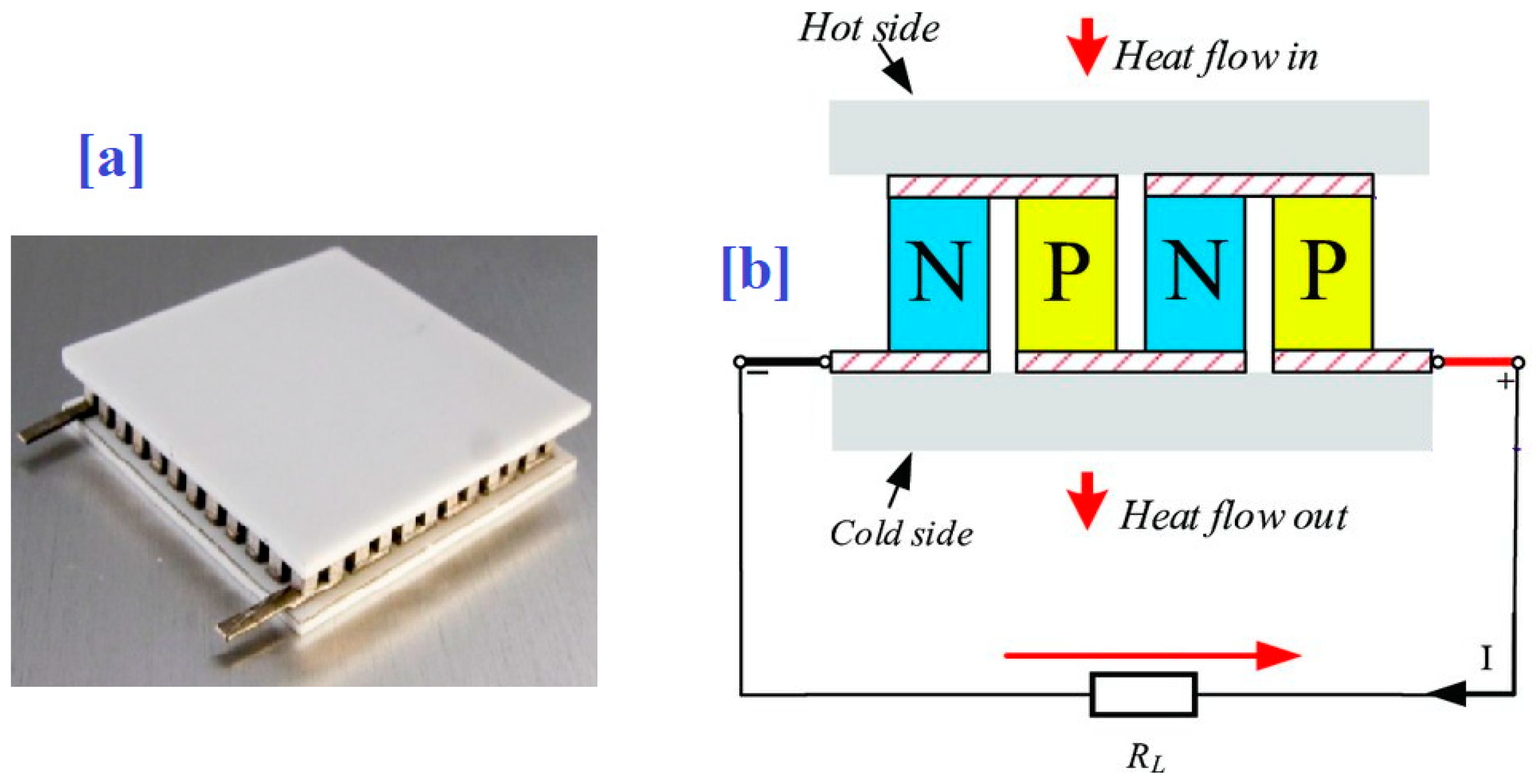
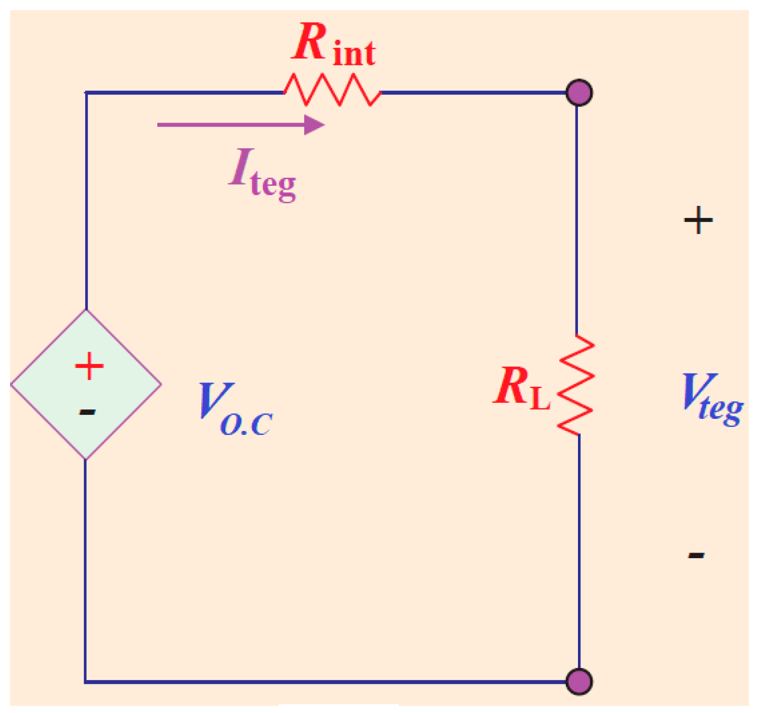
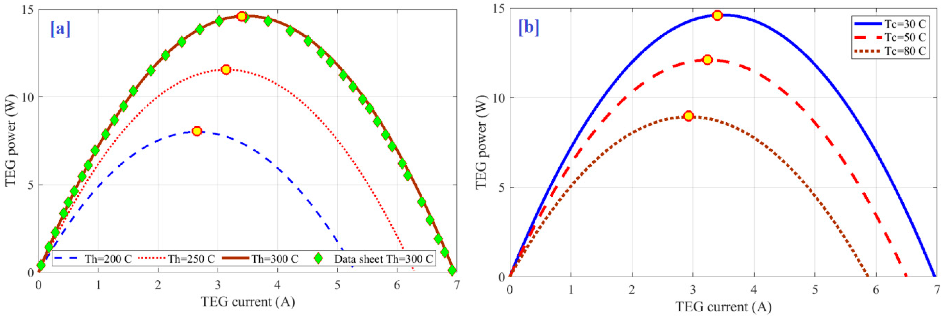
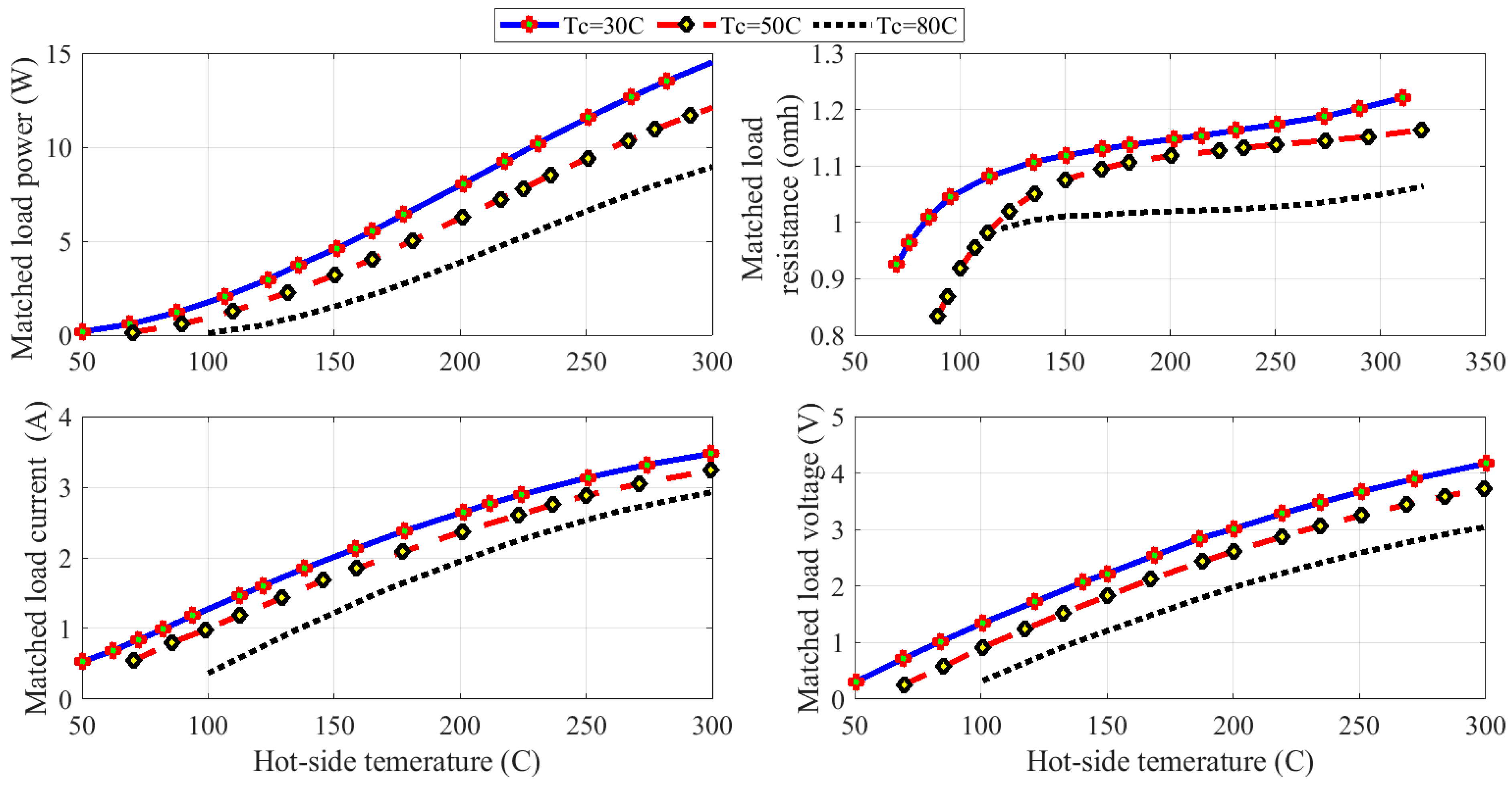
2. Modelling of Thermoelectric Generator
3. MRFO Algorithm
| Algorithm 1 Pseudo code of the proposed MRFO |
| 1: Input: set the MRFOs’ parameters: maximum number of iterations and agents. |
| 2: Compute the initial population with N solutions randomly |
| 4: Valuate the objective function of and assign the best solution (). |
| 5: for I = 1 : N do |
| 6: if rand <0.5 then |
| 7: if t/T < rand then |
| 8: Apply Equation (10) to update . |
| 9: else |
| 10: Apply Equation (13) to update . |
| 11: end if |
| 12: else |
| 13: Apply Equation (7) to update . |
| 14: end if |
| 15: end for |
| 16: for i = 1 : N do |
| 17: Apply Equation. (14) to update . |
| 18: end for |
| 19: t = t + 1. |
| 20: until Stop criteria is met |
| 21: Return the best solution . |
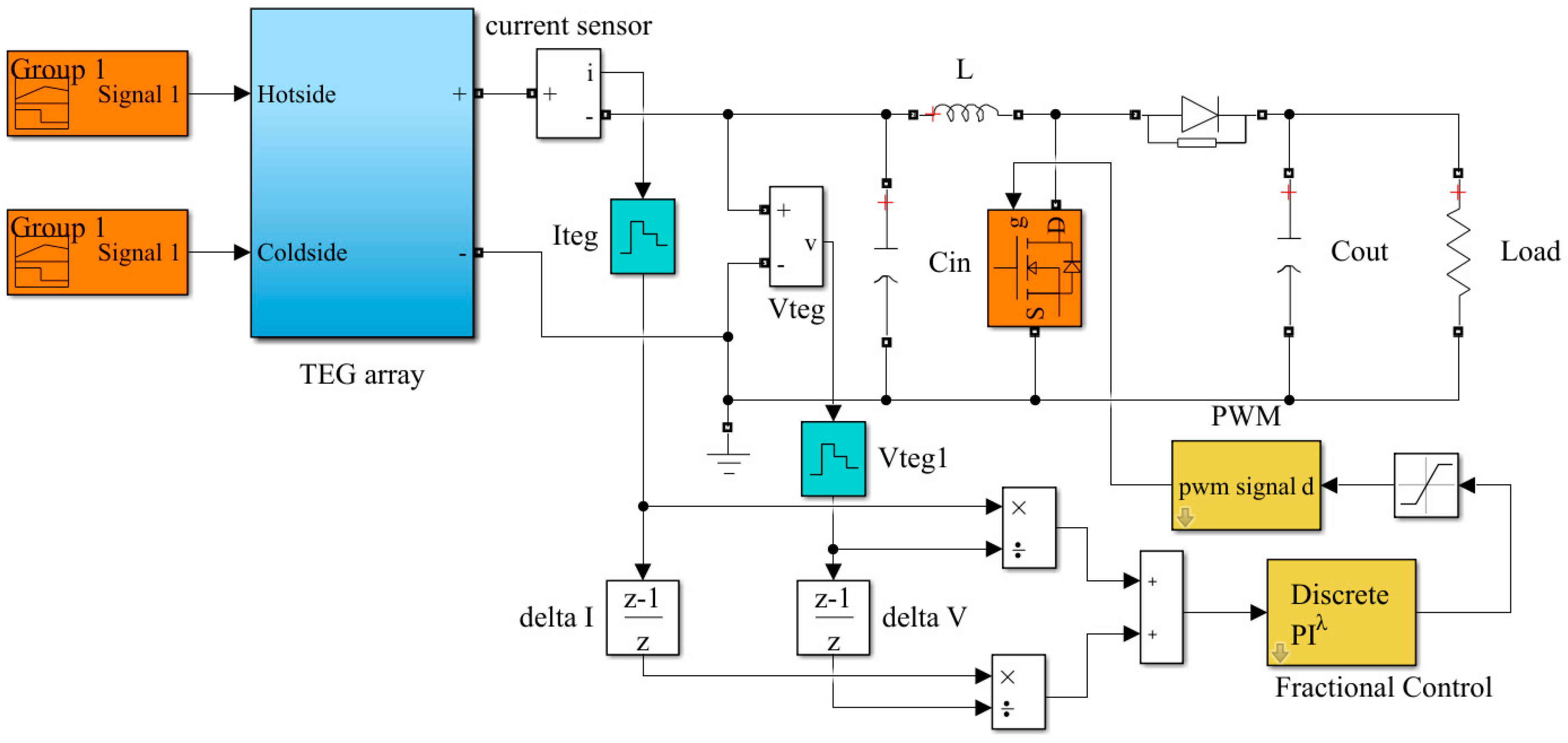
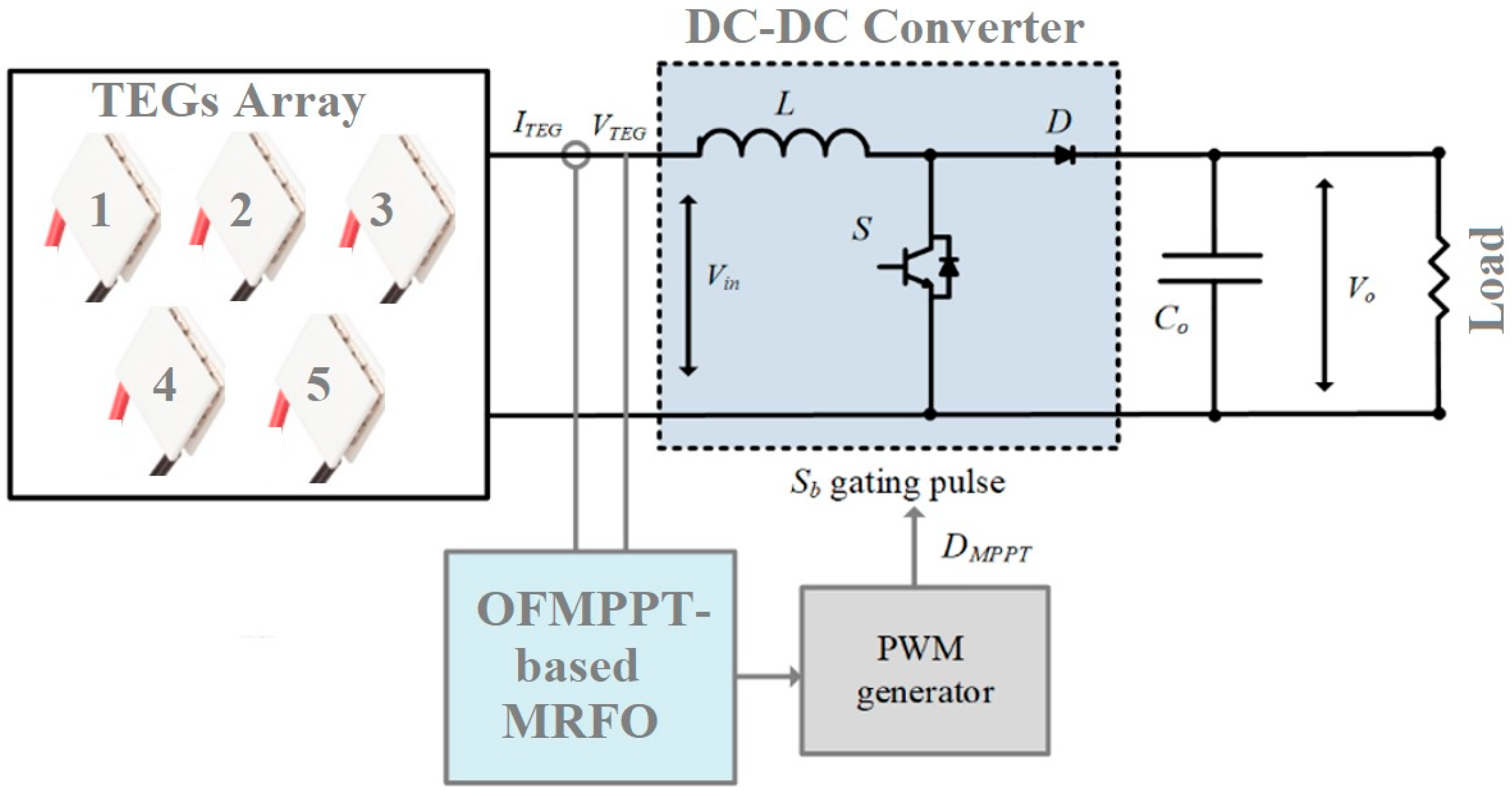
4. Optimized Fractional MPPT Strategy
5. Results and Discussion
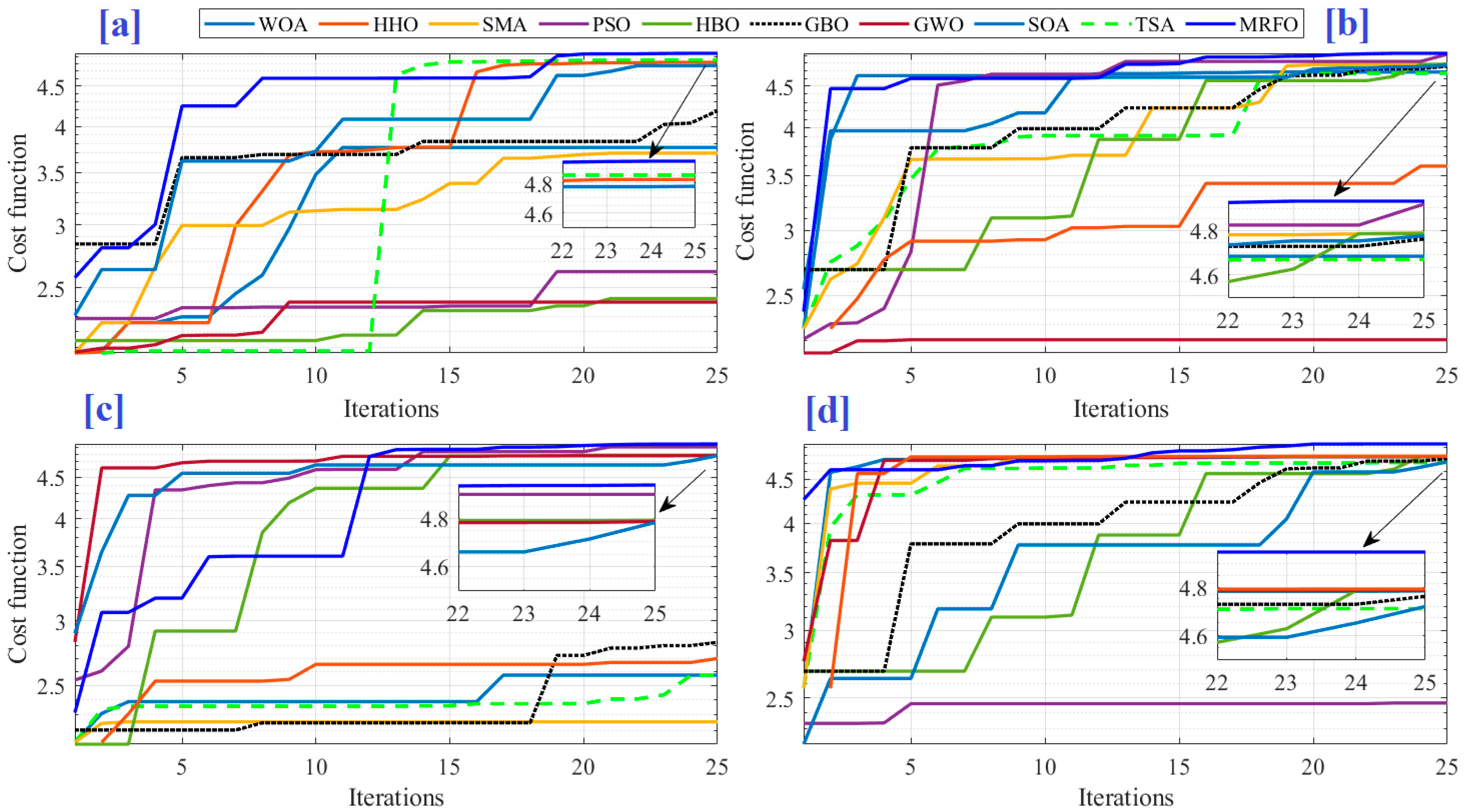
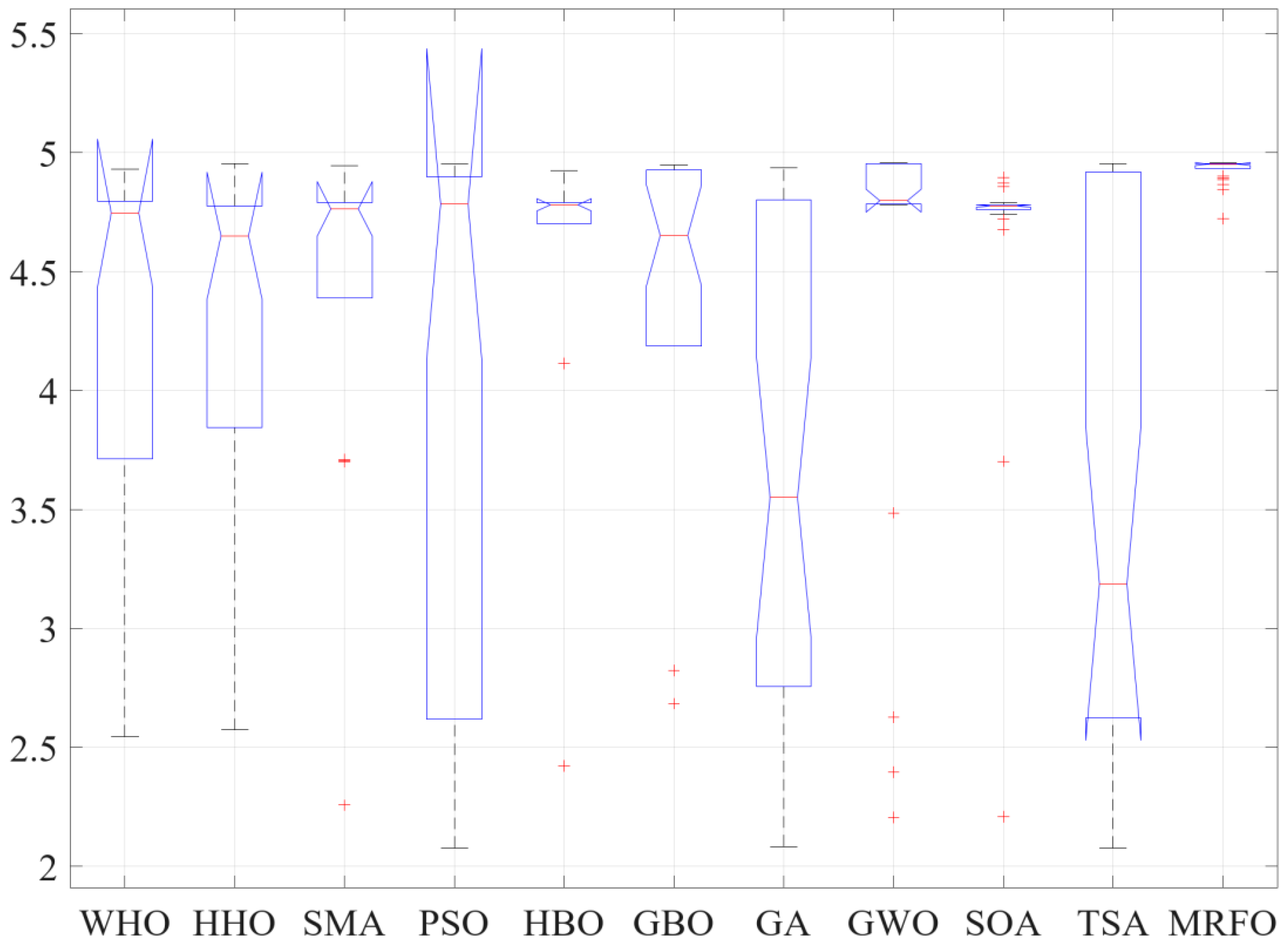
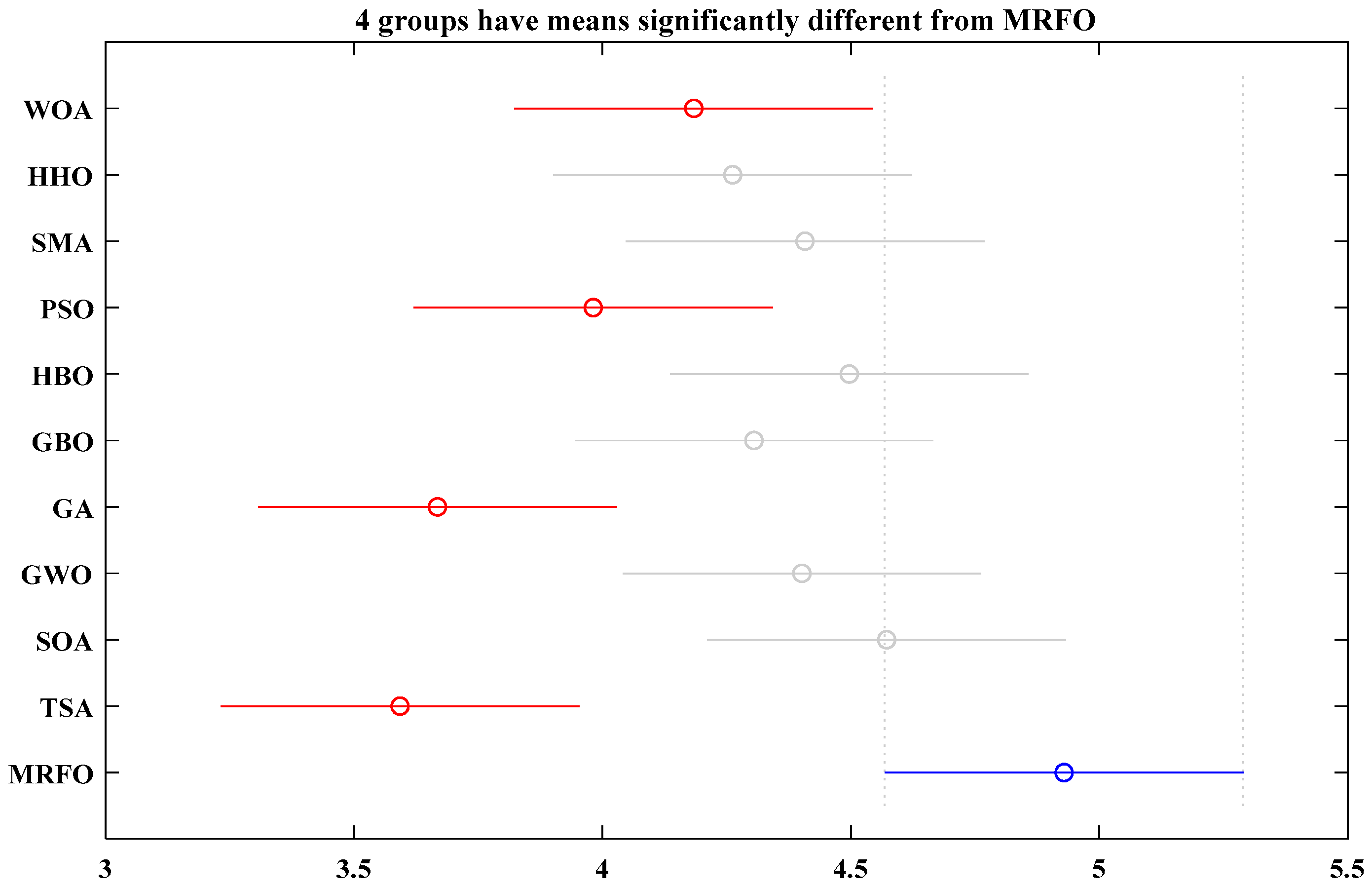
5.1. Evaluation of MRFO
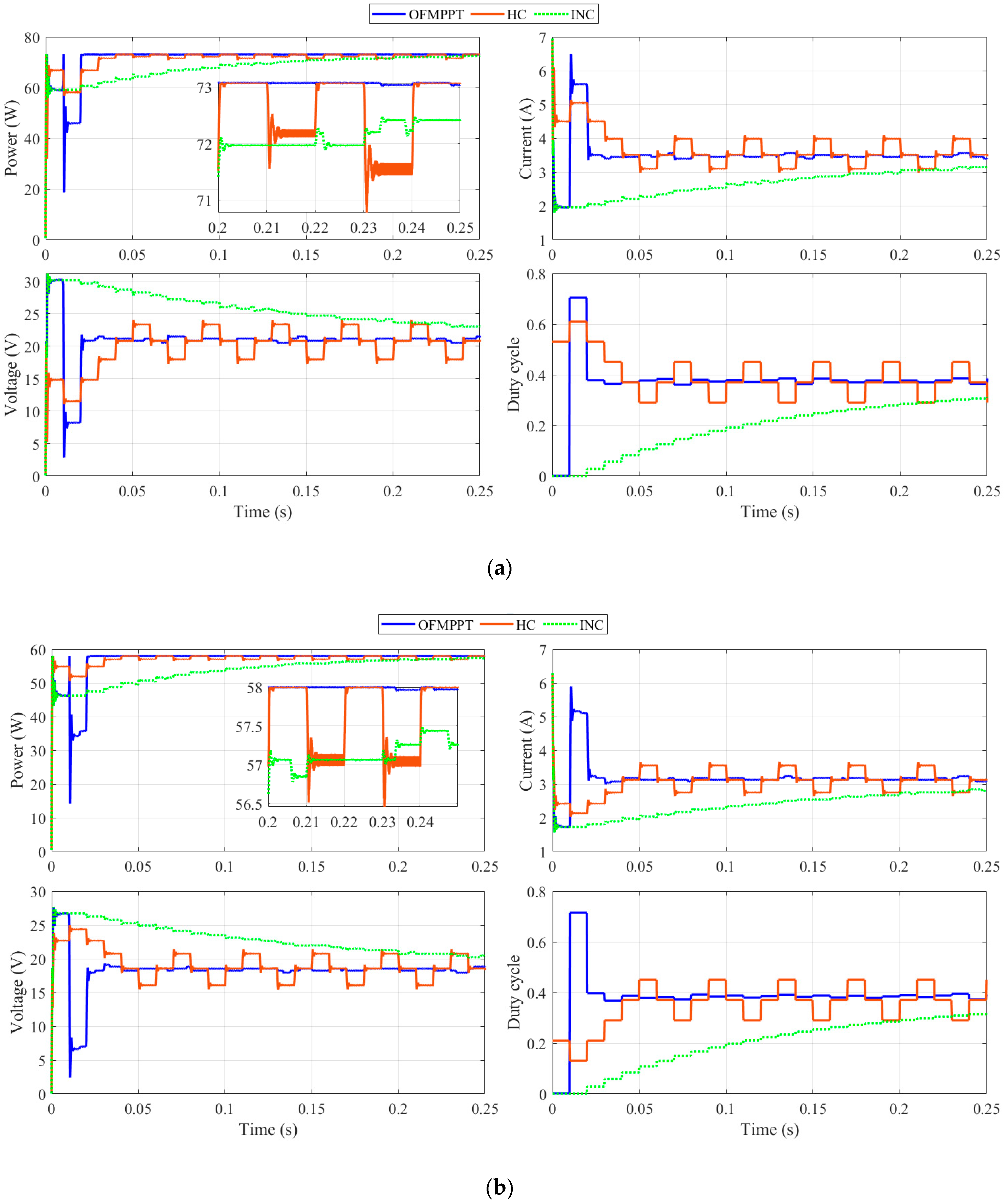
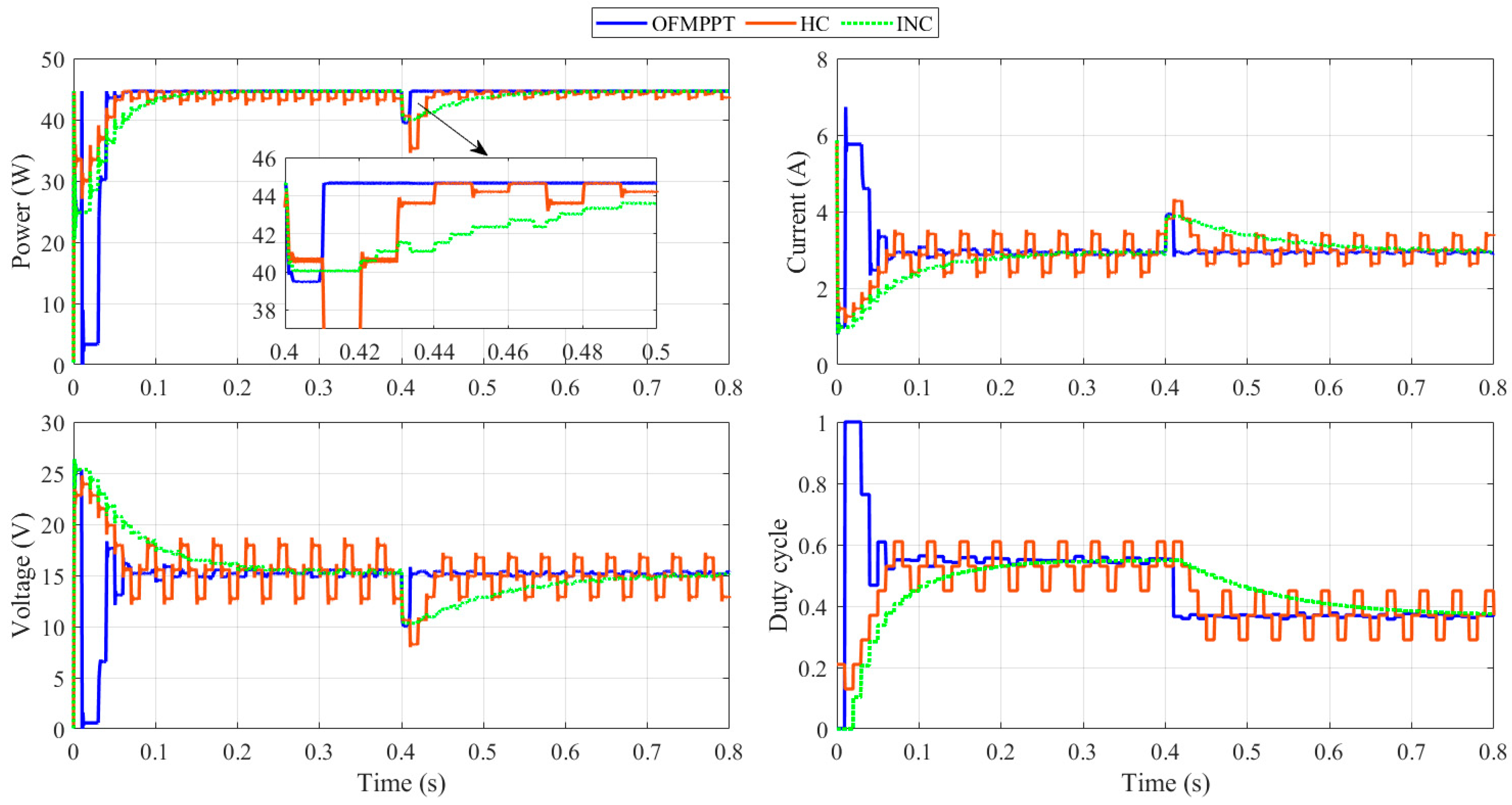
5.2. 1st Scenario
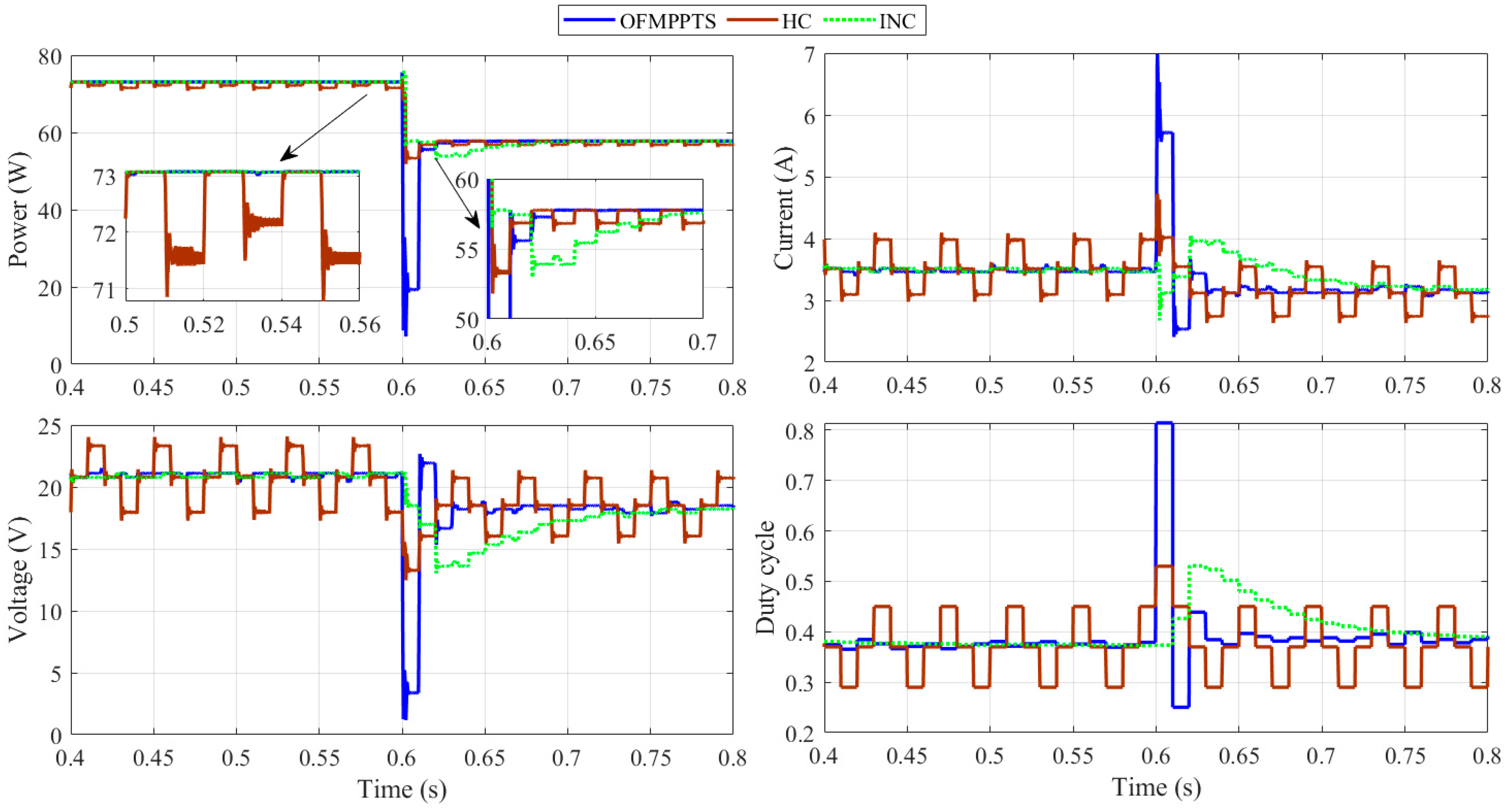
5.3. 2nd Scenario
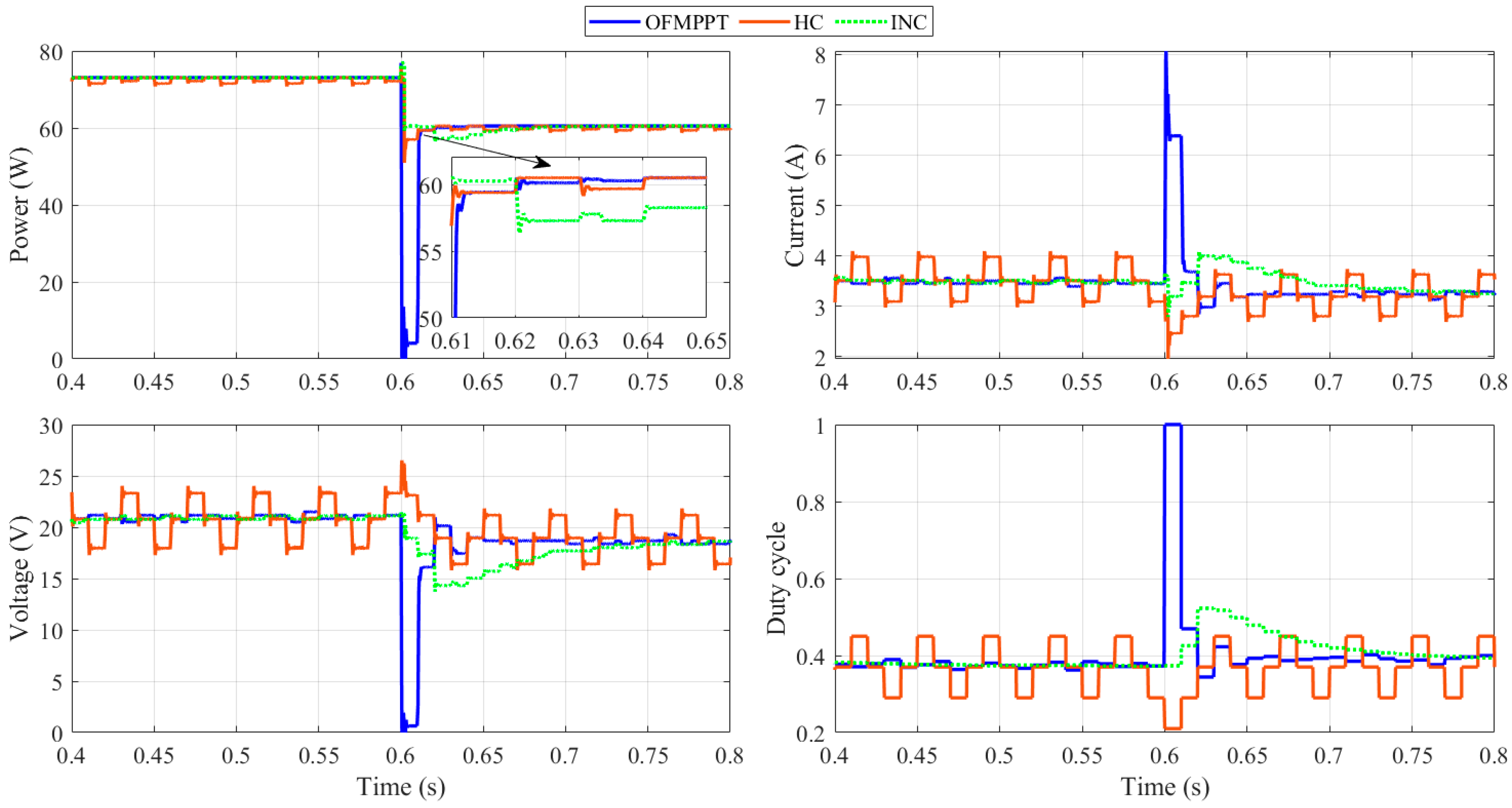
5.4. 3rd Scenario
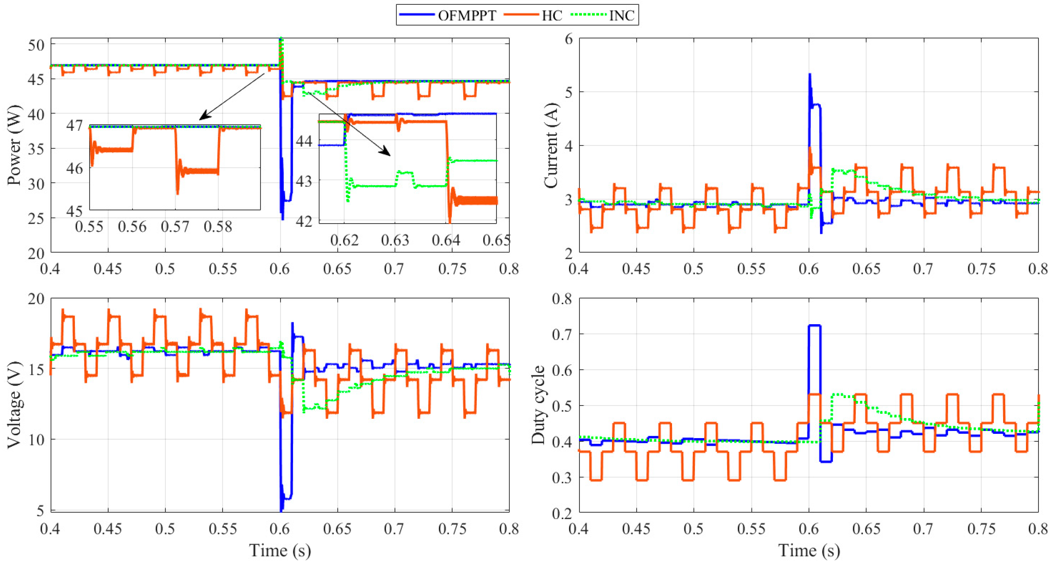
5.5. 4th Scenario
5.6. 5th Scenario, Change in the Load
6. Conclusions
Author Contributions
Funding
Institutional Review Board Statement
Informed Consent Statement
Data Availability Statement
Conflicts of Interest
References
- Shen, Z.-G.; Tian, L.-L.; Liu, X. Automotive exhaust thermoelectric generators: Current status, challenges and future prospects. Energy Convers. Manag. 2019, 195, 1138–1173. [Google Scholar] [CrossRef]
- Liu, X.; Deng, Y.; Li, Z.; Su, C. Performance analysis of a waste heat recovery thermoelectric generation system for automotive application. Energy Convers. Manag. 2015, 90, 121–127. [Google Scholar] [CrossRef]
- Champier, D. Thermoelectric generators: A review of applications. Energy Convers. Manag. 2017, 140, 167–181. [Google Scholar] [CrossRef]
- Tang, S.; Wang, C.; Liu, X.; Su, G.; Tian, W.; Qiu, S.; Zhang, Q.; Liu, R.; Bai, S. Experimental investigation of a novel heat pipe thermoelectric generator for waste heat recovery and electricity generation. Int. J. Energy Res. 2020, 44, 7450–7463. [Google Scholar] [CrossRef]
- Patowary, R.; Baruah, D.C. Thermoelectric conversion of waste heat from IC engine-driven vehicles: A review of its application, issues, and solutions. Int. J. Energy Res. 2018, 42, 2595–2614. [Google Scholar] [CrossRef]
- Jena, S.; Kar, S.K. Employment of solar photovoltaic-thermoelectric generator-based hybrid system for efficient operation of hybrid nonconventional distribution generator. Int. J. Energy Res. 2020, 44, 109–127. [Google Scholar] [CrossRef]
- Lekbir, A.; Hassani, S.; Mekhilef, S.; Saidur, R.; Ab Ghani, M.R.; Gan, C.K. Energy performance investigation of nanofluid-based concentrated photovoltaic / thermal-thermoelectric generator hybrid system. Int. J. Energy Res. 2021, 45, 9039–9057. [Google Scholar] [CrossRef]
- Liu, C.; Ye, W.; Li, H.; Liu, J.; Zhao, C.; Mao, Z.; Pan, X. Experimental study on cascade utilization of ship’s waste heat based on TEG-ORC combined cycle. Int. J. Energy Res. 2020, 45, 4184–4196. [Google Scholar] [CrossRef]
- Mamur, H.; Ahiska, R. Application of a DC–DC boost converter with maximum power point tracking for low power thermoelectric generators. Energy Convers. Manag. 2015, 97, 265–272. [Google Scholar] [CrossRef]
- Torrecilla, M.C.; Montecucco, A.; Siviter, J.; Knox, A.R.; Strain, A. Novel model and maximum power tracking algorithm for thermoelectric generators operated under constant heat flux. Appl. Energy 2019, 256, 113930. [Google Scholar] [CrossRef]
- Torrecilla, M.C.; Montecucco, A.; Siviter, J.; Strain, A.; Knox, A.R. Transient response of a thermoelectric generator to load steps under constant heat flux. Appl. Energy 2018, 212, 293–303. [Google Scholar] [CrossRef] [Green Version]
- Yu, C.; Chau, K.T. Thermoelectric automotive waste heat energy recovery using maximum power point tracking. Energy Convers. Manag. 2009, 50, 1506–1512. [Google Scholar] [CrossRef]
- Verma, V.; Kane, A.; Singh, B. Complementary performance enhancement of PV energy system through thermoelectric generation. Renew. Sustain. Energy Rev. 2016, 58, 1017–1026. [Google Scholar] [CrossRef]
- Twaha, S.; Zhu, J.; Li, B.; Yan, Y.; Huang, K. Parameter analysis of thermoelectric generator/dc-dc converter system with maximum power point tracking. Energy Sustain. Dev. 2017, 41, 49–60. [Google Scholar] [CrossRef]
- Rezk, H.; Aly, M.; Al-Dhaifallah, M.; Shoyama, M. Design and Hardware Implementation of New Adaptive Fuzzy Logic-Based MPPT Control Method for Photovoltaic Applications. IEEE Access 2019, 7, 106427–106438. [Google Scholar] [CrossRef]
- Reddy, K.J.; Sudhakar, N. ANFIS-MPPT control algorithm for a PEMFC system used in electric vehicle applications. Int. J. Hydrogen Energy 2019, 44, 15355–15369. [Google Scholar] [CrossRef]
- Mohamed, M.A.; Diab, A.A.Z.; Rezk, H. Partial shading mitigation of PV systems via different meta-heuristic techniques. Renew. Energy 2019, 130, 1159–1175. [Google Scholar] [CrossRef]
- Rezk, H.; Eltamaly, A.M. A comprehensive comparison of different MPPT techniques for photovoltaic systems. Sol. Energy 2015, 112, 1–11. [Google Scholar] [CrossRef]
- Bayat, P.; Baghramian, A. A novel self-tuning type-2 fuzzy maximum power point tracking technique for efficiency enhancement of fuel cell based battery chargers. Int. J. Hydrogen Energy 2020, 45, 23275–23293. [Google Scholar] [CrossRef]
- Kanagaraj, N.; Rezk, H.; Behiri, M.R.G. A Variable Fractional Order Fuzzy Logic Control Based MPPT Technique for Improving Energy Conversion Efficiency of Thermoelectric Power Generator. Energies 2020, 13, 4531. [Google Scholar] [CrossRef]
- Salomon, R. Evolutionary algorithms and gradient search: Similarities and differences. IEEE Trans. Evol. Comput. 1998, 2, 45–55. [Google Scholar] [CrossRef]
- Ariyarit, A.; Kanazaki, M.; Bureerat, S. An approach combining an efficient and global evolutionary algorithm with a gradi-ent-based method for airfoil design problems. Smart Sci. 2020, 8, 14–23. [Google Scholar] [CrossRef]
- Rezk, H.; Ali, Z.M.; Abdalla, O.; Younis, O.; Gomaa, M.R.; Hashim, M. Hybrid Moth-Flame Optimization Algorithm and Incremental Conductance for Tracking Maximum Power of Solar PV/Thermoelectric System under Different Conditions. Mathematics 2019, 7, 875. [Google Scholar] [CrossRef] [Green Version]
- Twaha, S.; Zhu, J.; Yan, Y.; Li, B.; Huang, K. Performance analysis of thermoelectric generator using dc-dc converter with incremental conductance based maximum power point tracking. Energy Sustain. Dev. 2017, 37, 86–98. [Google Scholar] [CrossRef]
- Shanmugam, S.; Eswaramoorthy, M.; Veerappan, A.R. Modeling and Analysis of a Solar Parabolic Dish Thermoelectric Generator. Energy Sources Part A Recovery Util. Environ. Eff. 2014, 36, 1531–1539. [Google Scholar] [CrossRef]
- Zhao, W.; Zhang, Z.; Wang, L. Manta ray foraging optimization: An effective bio-inspired optimizer for engineering applications. Eng. Appl. Artif. Intell. 2020, 87, 103300. [Google Scholar] [CrossRef]
- Al-Dhaifallaha, M.; Nassefa, A.M.; Rezka, H.; Nisar, K.S. Maximum Power Point Tracking Converter Based on the Open-Circuit Voltage Method for Thermoelectric Generators. Solar Energy 2018, 159, 650–664. [Google Scholar]


| Parameter | WOA | HHO | SMA | PSO | HBO | GBO | GA | GWO | SOA | TSA | MRFO |
|---|---|---|---|---|---|---|---|---|---|---|---|
| Kp | 0.0332 | 0.03751 | 0.0391 | 0.03346 | 0.12091 | 0.02516 | 0.0332 | 0.03765 | 0.001 | 0.03517 | 0.03526 |
| Ki | 5.47598 | 6.97039 | 10 | 6.6776 | 10 | 6.55569 | 5.47598 | 8.43451 | 5.37608 | 6.80429 | 7.03875 |
| Λ | 0.9425 | 0.98175 | 1.05291 | 0.98458 | 0.90286 | 0.96783 | 0.9425 | 1.01008 | 0.96099 | 0.98341 | 0.98753 |
| Best | 4.931 | 4.95502 | 4.94548 | 4.95252 | 4.92605 | 4.94796 | 4.93671 | 4.95599 | 4.89537 | 4.95493 | 4.95628 |
| Worst | 2.54544 | 2.57381 | 2.25665 | 2.07699 | 2.4211 | 2.6838 | 2.08277 | 2.206 | 2.20845 | 2.07699 | 4.72286 |
| Average | 4.184 | 4.26215 | 4.40775 | 3.98158 | 4.49684 | 4.30514 | 3.66791 | 4.40155 | 4.5721 | 3.59264 | 4.92934 |
| Median | 4.74639 | 4.65052 | 4.76375 | 4.78396 | 4.78075 | 4.65201 | 3.55039 | 4.79806 | 4.77588 | 3.18702 | 4.95199 |
| Variance | 0.67783 | 0.57425 | 0.49127 | 1.31103 | 0.52463 | 0.65678 | 1.0246 | 0.93066 | 0.43788 | 1.39508 | 0.00237 |
| STD | 0.8233 | 0.75779 | 0.70091 | 1.145 | 0.72431 | 0.81042 | 1.01223 | 0.96471 | 0.66172 | 1.18114 | 0.04867 |
| Efficiency | 84.42 | 85.99 | 88.93 | 80.33 | 90.73 | 86.86 | 74.01 | 88.81 | 92.25 | 72.49 | 99.46 |
| Run | WOA | HHO | SMA | PSO | HBO | GBO | GA | GWO | SOA | TSA | MRFO |
|---|---|---|---|---|---|---|---|---|---|---|---|
| 1 | 3.76259 | 4.82375 | 3.70032 | 2.61898 | 2.4211 | 4.18754 | 3.54552 | 2.39641 | 4.7769 | 4.85412 | 4.95179 |
| 2 | 4.92233 | 4.88977 | 3.71087 | 4.77512 | 4.89126 | 4.43418 | 2.33783 | 2.62759 | 4.76421 | 4.79322 | 4.94955 |
| 3 | 4.79096 | 4.71743 | 4.3898 | 4.91843 | 4.77634 | 4.54291 | 3.56027 | 4.95599 | 4.78037 | 2.87615 | 4.94118 |
| 4 | 4.36253 | 4.94213 | 3.7038 | 4.78067 | 4.92605 | 4.80777 | 3.55526 | 4.95568 | 4.77691 | 3.42849 | 4.9554 |
| 5 | 4.931 | 4.9209 | 4.94548 | 4.90829 | 4.11402 | 4.92813 | 4.80276 | 4.79064 | 4.67628 | 4.7906 | 4.95616 |
| 6 | 4.79074 | 4.95502 | 4.599 | 2.81205 | 4.79108 | 2.82378 | 4.07527 | 4.78124 | 4.77337 | 4.95493 | 4.95302 |
| 7 | 4.85854 | 4.67945 | 3.70329 | 4.95252 | 4.78655 | 2.6838 | 4.53135 | 4.78707 | 4.7724 | 4.91833 | 4.95555 |
| 8 | 3.00088 | 3.22244 | 3.7091 | 4.82095 | 4.77579 | 4.93421 | 4.92039 | 4.83516 | 4.77703 | 2.94555 | 4.89275 |
| 9 | 4.68338 | 4.66883 | 4.7897 | 4.92296 | 4.78516 | 4.76111 | 3.43438 | 2.20606 | 4.77487 | 3.59444 | 4.93629 |
| 10 | 4.92327 | 4.71838 | 4.43459 | 4.80228 | 4.70101 | 4.94796 | 2.82891 | 4.78465 | 4.78064 | 2.16985 | 4.95485 |
| 11 | 3.72151 | 2.77701 | 4.65532 | 2.56349 | 2.4211 | 4.18754 | 4.89911 | 4.95587 | 4.77763 | 2.62508 | 4.86738 |
| 12 | 4.79505 | 4.77647 | 4.84489 | 4.78725 | 4.89126 | 4.43418 | 2.56189 | 4.9519 | 4.78125 | 2.07699 | 4.93492 |
| 13 | 3.71209 | 3.8439 | 4.74149 | 2.07699 | 4.77634 | 4.54291 | 4.93671 | 4.78468 | 4.78933 | 4.94024 | 4.95539 |
| 14 | 3.71254 | 4.08623 | 4.79641 | 4.79427 | 4.92605 | 4.80777 | 4.84729 | 4.95289 | 4.78227 | 2.18836 | 4.94362 |
| 15 | 4.78558 | 4.90784 | 4.7905 | 2.85116 | 4.11402 | 4.92813 | 4.87949 | 3.48553 | 4.7839 | 4.9541 | 4.84592 |
| 16 | 2.57422 | 2.57381 | 2.25665 | 4.90264 | 4.79108 | 2.82378 | 2.75611 | 4.78623 | 4.78269 | 2.69843 | 4.95592 |
| 17 | 4.74639 | 3.75485 | 4.78059 | 2.16345 | 4.78655 | 2.6838 | 4.91324 | 4.78717 | 4.85734 | 2.36666 | 4.90192 |
| 18 | 4.87047 | 4.63222 | 4.76375 | 4.83033 | 4.77579 | 4.93421 | 4.79966 | 4.80548 | 4.76201 | 4.95434 | 4.95334 |
| 19 | 4.78364 | 4.70971 | 4.78641 | 2.46626 | 4.78516 | 4.76111 | 4.5772 | 4.78566 | 4.71861 | 4.79155 | 4.95089 |
| 20 | 2.54544 | 4.60113 | 4.85726 | 4.94 | 4.70101 | 4.94796 | 3.0091 | 4.95598 | 4.75494 | 2.63098 | 4.95615 |
| 21 | 3.72151 | 2.77701 | 4.65532 | 4.72675 | 2.4211 | 4.18754 | 2.71204 | 4.81295 | 4.87138 | 2.62508 | 4.9477 |
| 22 | 4.79505 | 4.77647 | 4.84489 | 2.53759 | 4.89126 | 4.43418 | 2.8974 | 4.78751 | 4.7795 | 2.07699 | 4.88628 |
| 23 | 3.71209 | 3.8439 | 4.74149 | 4.94008 | 4.77634 | 4.54291 | 4.60893 | 4.95348 | 4.74162 | 4.94024 | 4.95628 |
| 24 | 3.71254 | 4.08623 | 4.79641 | 4.83965 | 4.92605 | 4.80777 | 2.83561 | 4.95488 | 4.89537 | 2.18836 | 4.95241 |
| 25 | 4.78558 | 4.90784 | 4.7905 | 2.45962 | 4.11402 | 4.92813 | 2.60601 | 4.95086 | 2.20845 | 4.9541 | 4.9522 |
| 26 | 2.57422 | 2.57381 | 2.25665 | 4.86354 | 4.79108 | 2.82378 | 2.38001 | 4.91246 | 3.7021 | 2.69843 | 4.88626 |
| 27 | 4.74639 | 3.75485 | 4.78059 | 2.206 | 4.78655 | 2.6838 | 4.84819 | 2.206 | 4.77138 | 2.36666 | 4.95258 |
| 28 | 4.87047 | 4.63222 | 4.76375 | 4.89751 | 4.77579 | 4.93421 | 2.19438 | 4.95381 | 4.77222 | 4.95434 | 4.72286 |
| 29 | 4.78364 | 4.70971 | 4.78641 | 2.65152 | 4.78516 | 4.76111 | 2.08277 | 4.93654 | 4.76955 | 4.79155 | 4.95572 |
| 30 | 2.54544 | 4.60113 | 4.85726 | 4.63692 | 4.70101 | 4.94796 | 3.10016 | 2.206 | 2.20845 | 2.63098 | 4.95598 |
| R+ | 456 | 458 | 463 | 449 | 458 | 435 | 452 | 392 | 463 | 438 | |
| R− | 9 | 7 | 2 | 16 | 7 | 30 | 13 | 73 | 2 | 27 | |
| p-Value | 4.2858 × 10⁻⁶ | 3.5152 × 10⁻⁶ | 2.1266 × 10⁻⁶ | 8.46608 × 10⁻⁶ | 3.51523 × 10⁻⁶ | 3.112312 × 10⁻⁵ | 6.339135 × 10⁻⁶ | 0.0010356 | 2.126636 × 10⁻⁶ | 2.37044 × 10⁻⁵ | |
| H | No | No | No | No | No | No | No | No | No | No | |
| Friedman Aver Rank | 6.6666 | 7.2333 | 6.4666 | 6.5833 | 5.7666 | 5.9333 | 7.6333 | 4.6833 | 6.3333 | 6.7667 | 1.9333 |
| (8) | (10) | (6) | (7) | (3) | (4) | (11) | (2) | (5) | (9) | (1) |
| Source | SS | df | MS | F | p-Value > F |
|---|---|---|---|---|---|
| Columns | 45.73 | 10 | 4.57304 | 6.06 | 1.92249 × 10⁻⁸ |
| Error | 240.792 | 319 | 0.75483 | ||
| Total | 286.522 | 329 |
| Scenario | Time Step | Th °C | Tc °C | Load | Vm (V) | Im (A) | Pm (W) |
|---|---|---|---|---|---|---|---|
| 1st scenario | From 0.0 s to 0.25 s | 300 °C | 30 °C | 15 Ω | 21 | 3.4 | 73 |
| From 0.0 s to 0.25 s | 250 °C | 18.36 | 3.14 | 57.86 | |||
| 2nd scenario | From 0.4 s to 0.6 s | 300 °C | 30 °C | 15 Ω | 21 | 3.4 | 73 |
| From 0.6 s to 0.8 s | 250 °C | 18.36 | 3.14 | 57.86 | |||
| 3rd scenario | From 0.4 s to 0.6 s | 300 °C | 30 °C | 15 Ω | 21 | 3.4 | 73 |
| From 0.6 s to 0.8 s | 50 °C | 18.63 | 3.24 | 60.57 | |||
| 4th scenario | From 0.4 s to 0.6 s | 250 °C | 50 °C | 15 Ω | 16.25 | 2.88 | 47 |
| From 0.6 s to 0.8 s | 300 °C | 80 °C | 15.22 | 2.93 | 44.85 | ||
| 5th scenario | From 0.0 s to 0.25 s | 300 °C | 30 °C | 25 Ω | 15.22 | 2.93 | 44.85 |
Publisher’s Note: MDPI stays neutral with regard to jurisdictional claims in published maps and institutional affiliations. |
© 2021 by the authors. Licensee MDPI, Basel, Switzerland. This article is an open access article distributed under the terms and conditions of the Creative Commons Attribution (CC BY) license (https://creativecommons.org/licenses/by/4.0/).
Share and Cite
Fathy, A.; Rezk, H.; Yousri, D.; Houssein, E.H.; Ghoniem, R.M. Parameter Identification of Optimized Fractional Maximum Power Point Tracking for Thermoelectric Generation Systems Using Manta Ray Foraging Optimization. Mathematics 2021, 9, 2971. https://0-doi-org.brum.beds.ac.uk/10.3390/math9222971
Fathy A, Rezk H, Yousri D, Houssein EH, Ghoniem RM. Parameter Identification of Optimized Fractional Maximum Power Point Tracking for Thermoelectric Generation Systems Using Manta Ray Foraging Optimization. Mathematics. 2021; 9(22):2971. https://0-doi-org.brum.beds.ac.uk/10.3390/math9222971
Chicago/Turabian StyleFathy, Ahmed, Hegazy Rezk, Dalia Yousri, Essam H. Houssein, and Rania M. Ghoniem. 2021. "Parameter Identification of Optimized Fractional Maximum Power Point Tracking for Thermoelectric Generation Systems Using Manta Ray Foraging Optimization" Mathematics 9, no. 22: 2971. https://0-doi-org.brum.beds.ac.uk/10.3390/math9222971