1. Introduction
Unmanned aerial vehicle (UAV) networks connect the gap among spaceborne, airborne, and ground-based remote sensing data. Its characteristics of lightweight and low price enable affordable observations with very high spatial and temporal resolutions. The developments in remote sensing technology and the resultant considerable developments in the temporal, spatial, and spectral resolutions of remotely sensed data, as well as the remarkable improvements in information and communication technologies (ICT) based on data transmission, storing, management, and integration capabilities, are drastically changing the way they observed the Earth [
1]. The most important application of remote sensing data is to observe the Earth, and most main concern in Earth monitoring is observing the changes in land cover. Detrimental modifications in land-use and land-cover (LULC) are the primary contributor to dramatic climate changes, terrestrial biodiversity losses, and harms to the ecosystem [
2]. Observing the gradual changes in the land cover assist in avoiding and predicting hazardous events and natural disasters. However, this observation is labor-intensive and very expensive, and it can be highly constrained to first-world countries. The accessibility of higher resolution remote sensing data on a continuous temporal basis could be much more efficient to automatically extract land covers and on-Earth objects and monitor and map their modifications.
Recently, LULC classification with remote sensing imagery plays a significant part in several applications such as biological resource (habitat quality, wetlands, and fragmentation), agricultural practice (nutrient management, cropping patterns, riparian zone buffers, and conservation easements), land use planning (incentives, growth trends, policy regulations, and suburban sprawl), and forest management (stand-quality, health, resource inventory, harvesting, and reforestation) [
3]. Land use refers to the purposes the land services, and land cover refers to the surface covers on the ground, either bare, soil vegetation, water, urban infrastructure, etc.; it does not determine the use of land, and that might be distinct for lands with the similar cover types [
4]. LULC assessment is much needed in planning, sustaining, and monitoring the use of natural resources. In fact, LULC classification directly affects water, atmospheric, and soil erosion, when it is not directly related to global environmental challenges [
5]. To this end, the remote sensing imagery and its processing have helped in delivering advanced and largescale data on surface conditions. For years, techniques mainly based on pixel or object analysis have been used for LULC classification. In fact, different from the pixel-based method that categorizes the pixel based on their spectral data, the object-based algorithm encloses semantic data, not in a single-pixel but a group of pixels with the same features, like shape, color, texture, and brightness. Both spatial and spectral resolution is used in this latter case for segmenting and later categorize image features into useful objects [
6]. From the resultant segment, a homogeneous image object is extracted according to the local contrast. This homogeneous object is later categorized into conventional classification methods like fuzzy classification logic, nearest neighbor, and knowledge-based methods.
Deep learning (DL) demonstrates very promising changes [
7], object detection, LULC classifications, and scene classifications. A multilayer artificial convolutional neural network (CNN) allows automatic extraction of higher-level features from a labeled image. Using convolution kernels at multilevel functioning on upper-level feature map, the higher level feature is hierarchically extracted by the network. The backpropagation approach assists CNN alter its network parameter manually. The higher generalization capability of CNN outstands another machine learning model and make CNN the more mature and extensively employed deep learning frameworks. CNN-based land cover classification always follows a patch-based strategy [
8]. The patch-based approach employs a moving window with a fixed size on each pixel to generate overlapping patches [
9]. Then patches are fed into a CNN, which is composed of two functional parts. The first part of the CNN consists of pooling and multiple stacked convolution layers that are employed for feature extraction. The second part is usually implemented by a stack of fully connected layers with the SoftMax layer at an end to generate a probability distribution over different classes.
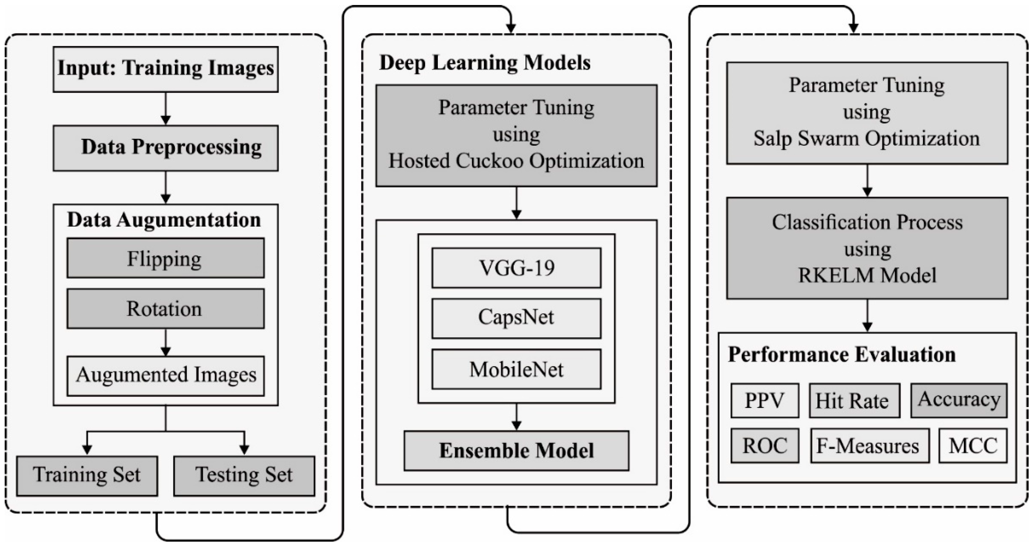
This paper proposes an ensemble of DL-based multimodal land cover classification (EDL-MMLCC) models using PlanetScope imagery. The EDL-MMLCC technique involves median filtering-based preprocessing and data augmentation. Moreover, an ensemble of feature extraction models using VGG-19, Capsule Network (CapsNet), and MobileNet is carried out. These three DL models are chosen due to faster training speed, fewer training samples per time, and higher accuracy. Furthermore, the hyperparameter optimizer using hosted cuckoo optimization (HCO) algorithm is derived. Lastly, the salp swarm algorithm (SSA) with regularized extreme learning machine (RELM) classifier is applied for land cover classification. These models are trained using an Amazon dataset from the Kaggle repository, and the results are investigated under several aspects.
2. Existing Land Cover Classification Models
Pan et al. [
10] proposed a CNN-based multispectral LiDAR land cover classification architecture and analyzed its optimum parameter for improving classification performance. Initially, this method pre-processes the multispectral three-dimensional LiDAR data to two-dimensional images. Then, CNN models are created using seven basic functional layers, and its hyperparameters are widely optimized and discussed. Kwan et al. [
11] explored the efficiency of two CNN-based DL models for land cover classification by means of five bands (RGB + NIR + LiDAR) and four bands (RGB + NIR), whereas this constrained amount of image bands is increased by the EMAP method. Zhang et al. [
12] proposed a state-of-the-art MLCG-OCNN algorithm. A feature fusing OCNN, include the object contour preserving mask approach using the supplement of object deformation coefficients, is presented for precise object discrimination by simultaneously learning higher-level features from geometric characteristics, object-level contextual information, and independent spectral patterns. Next, pixel-level contextual guidance is employed for additionally improving the per-object classification result.
In Rajendran et al. [
13], a hybrid feature optimization model and DL classifiers are presented for improving the performances of LULC classification, helps to forecast wildlife habitat, haphazard elements, deteriorating environment quality, and so on. LULC classifications are measured by Eurosat, Sat 4and Sat 6 datasets. Afterward, the election of remote sensing image, normalization and histogram equalization method is employed for improving the quality of an image. Next, a hybrid optimization is achieved through the use of the LGBPHS model, the HOG and Haralick texture feature, for extracting features from the elected image. Then, a human group-based PSO method is used for selecting an optimum feature, that advantages are ease of implementation and fast convergence rate. Afterward, electing an optimum feature value, LSTM networks are used for classifying the LULC class.
Chatterjee et al. [
14] proposed an unsupervised learning method for clustering hybrid polarimetric SAR image and dual-polarized SAR image with the deep structure. They employ the feature extraction layer of the VGG16 models using the BN model, i.e., trained by smaller patches acquired in the hybrid polarimetric SAR image. It employs an Adam, an adaptive learning rate optimization algorithm and entropy-based loss function, to train. Generally, the patches are divided into three kinds: double bounce, surface, and volume determined by the reference to the SAR scattering features. Moreover, they categorize volume to agricultural crop fields and dense forest regions. In Mboga et al. [
15], a fully convolution method is explored by taking into account the two network frameworks with district approaches of using contextual data: one employed atrous convolution layer without down-sampling, where the next network contains down-sampling and learned up-sampling convolution layer (U-NET). The network is trained for detecting three fundamental types: buildings, low vegetation class, higher vegetation, and a mixed class of bare land.
Moon et al. [
16] measured the precision of land cover classification through NN methods with higher resolution KOMPSAT-3 satellite imagery. Afterward attaining satellite imagery of coastal regions nearer Gyeongju City, training data have been generated. Also, the land cover has been categorized into DNN, SVM, and ANN methods for the three components of vegetation, land, and water. Later, the precision of classification results was quantitatively measured by an error matrix: the results with DNN models exhibited an accuracy of 92.0%. Aspri et al. [
17] considered a new multimodal DNN that depends on the CNN structure and examine many methods for optimizing its performances while training is performed on Apache Spark Clusters. They estimate the performances of distinct frameworks through the metrics of processing power and network traffic, consider the case of land cover classification from remote sensing observation.
3. The Proposed Model
In this study, a new EDL-MMLCC technique is derived for UAV networks using PlanetScope imagery. The EDL-MMLCC technique involves data preprocessing, data augmentation, ensemble DL based feature extraction, and SSA-RELM based classification. The HCO and SSA algorithms are derived to tune the parameters of the DL and RELM models respectively.
Figure 1 depicts the overall process of EDL-MMLCC model. The working of these modules is elaborated in the following sections.
3.1. Data Preprocessing and Augmentation
At the initial stage, the data preprocessing take place to improve the quality of the image using the median filtering (MF) technique. It is defined as a nonlinear signal processing model that is based on the current statistics. The inaccurate digital images can be modified by median values of neighborhoods which are named as masks. The pixel is graded for gray level, and median scores of a group have been saved to replace the incorrect values. The MF results are defined as
, in which
represents the actual as well as final images correspondingly,
defines the 2D mask: with the size of
such that
, and so on. The mask may be of any shape like a cross, linear, circular, square, etc. As MF is a nonlinear filter, the numerical examination is highly difficult for images with arbitrary noise [
18]. When the image has been assigned to noise below standard distribution, zero mean, noise variances of MF would be defined by,
where
defines the input noise power,
denotes the size of MF,
means the performance of noise intensity. Followed by, the noise variance of average filtering is denoted by
The comparison of (1) and (2) defines that the MF functions are based on two objectives: noise distribution and a mask’s size. The MF performs the noise elimination, which is considerable when compared to average filtering. Hence, for impulse noise, and narrow pulse is distant, and when the pulse width is lower when compared to , the MF is highly efficient. The function of MF is to maximize while the MF method is integrated with the average filtering model. Next, the data augmentation process is carried out in three levels, namely flipping and rotation.
3.2. Ensemble of DL Based Feature Extraction
Three DL models are passed into the ensemble learning process during the feature extraction process to generate the final output.
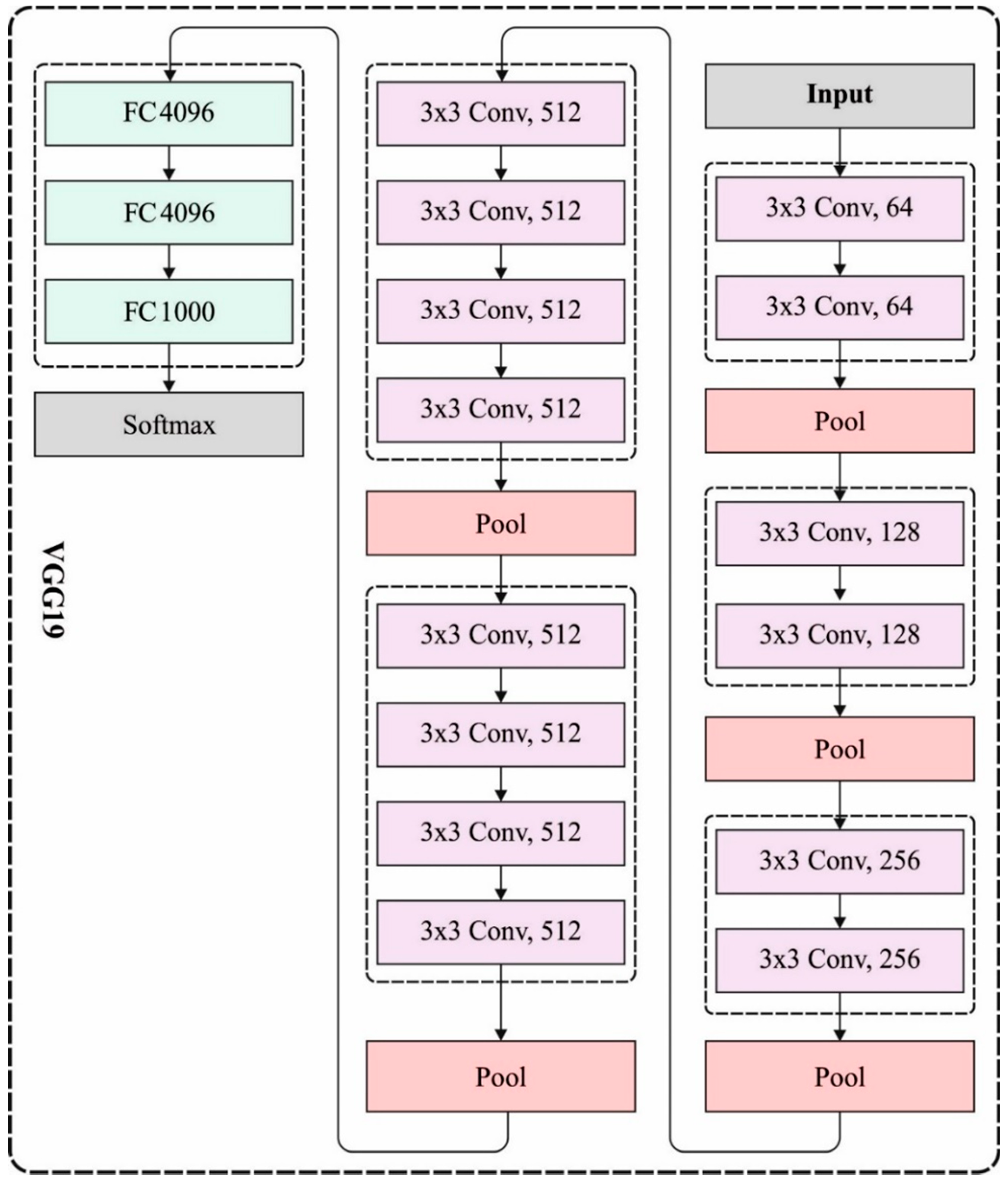
3.2.1. VGG19 Model
The VGGNet is a DNN with a multi-layered function. The VGGNet is dependent upon the CNN technique and has been implemented on ImageNet datasets. The VGG-19 has been helpful because of its simplicity, as
convolution layers have been attached on the top for increasing depth levels. During the training stage, convolution layers are utilized for the feature extraction and
-pooling layers connected to few convolution layers for reducing the feature dimensional. During the primary convolution layer, 64 kernels (
filter size) are executed to feature extraction in the input image. FC layers are utilized for preparing the feature vectors.
Figure 2 showcases the framework of VGG-19 model. The developed feature vector is more exposed to PCA as well as SVD for dimensional decrease and the feature selective of image data to optimum classifier outcomes. Reducing the extremely dimensionality data utilizing PCA as well as SVD is an important task [
19]. The PCA and SVD are further helpful it can be nearer and numerically further stable than other decrease approaches. Eventually, during the testing stage, 10-fold CV has been executed for classifying the DR images dependent upon the softmax activation approach. The efficiency of the presented VGG-19 based model is related to other feature extraction frameworks containing AlexNet as well as SIFT. The AlextNet has been a multi-layered feature extraction framework utilized from CNN. The SIFT has been a standard feature extraction approach established by Mansour for detecting the local feature of the input images from the domain of computer vision.
3.2.2. MobileNet Model
The MobileNet depends on a streamlined structure that employs depthwise separable convolution followed by pointwise convolutions for building a lightweight DNN model. The SSD MobileNet V2 architecture was employed in this study. The single-shot detector (SSD) model’s aim is to forecast bounding box location and classify this box in a single network. The SSD uses a modified VGG-16architecture pre-trained on the ImageNet as its backbone, with further convolution feature layers with progressively decreasing size. VGG-16 is a generally employed base feature extractor with sixteen layers of weight. ImageNet is a huge visual dataset for visual object detection software research. The MobileNetV2 uses only a single convolution network applied to each channel of the input image and slides the weighted sum to the following pixel. It includes two novel features, including short connections between bottlenecks and linear bottlenecks between layers, compared with MobileNetV1 [
20]. The MobileNetV2 has two types of block, one with a stride of two for downsizing and the other residual block with a stride of one.
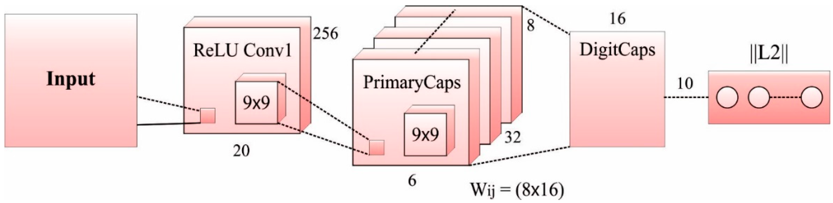
3.2.3. CapsNet Model
CapsNets refers to an entirely new kind of DL architecture that tries to conquer the limitations and drawbacks of CNN models, like losing valuable information and lacking the precise concept of an entity at the time of
pooling. A standard CapsNet (
Figure 3) is shallower, with three layers: DigitCaps, Convld, and PrimaryCaps layers. The capsule-based demonstration of a collection of hidden neurons, where probability, as well as the property of the hidden feature, can be captured. In this instance, CapsNet was strong to affine conversion and less training data. Additionally, CapsNets have resulted in certain breakthroughs associated with spatial hierarchies among features. A capsule represents a set of neurons [
21]. The activity of neurons surrounded in a dynamic capsule represents the distinct features of a certain entity. Since the length of output vectors represent the possibility of existence, an output capsule is calculated by non-linear squashing functions:
where as
represents the vector output of capsule
and
denotes the overall input. The non-linear squashing function is an activation function for ensuring that the short vector gets shrunk to nearly zero length and the longer vector gets shrunk to a certain length regarding
The overall inputs to a capsule
is attained by multiplying the output
of a capsule using a weight matrix
, that represents a weighted amount over each forecasted vector from the capsule in the below layers. Now,
represents a coupling coefficients, i.e., defined as the iterative dynamic routing procedure:
where as
&
represents the
prior likelihoods among 2 coupled capsules. The whole length of output vectors represents the forecasted likelihood. An individual margin loss
per capsule,
is expressed as follows
In which , and denotes three free variables by default. enable down weighting of loss and help to ensure latter convergences.
3.2.4. Ensemble Process
The ensemble process attempts to increase the performance of the DL model for the classification of cloud, shade, and land cover kinds. An ensemble model is used with 3 models (that is MobileNet, VGG-19, and CapsNet) where all models are trained to implement multilabel predictions of class. Ridge regression with the weight penalty hyper-parameter set is used to one to integrate the scores from the three frameworks to a last binary prediction of all the labels. The score from all the models are integrated into ensemble score by resolving the ridge regression problems:
Now
is the
with three matrices that have the probability through three frameworks for a label
. Afterward resolving
, the vector of regression weight, the ensemble score for label
is represented as
A predictive threshold is established by enhancing
of all the labels with an arbitrary optimization [
22]. Particularly, they employed an iterative method in which proposals for novel thresholds are made from a standard distribution using standard deviation equivalent to
and center on the present optimal threshold. Proposals are accepted when they result in a high for each label
. Now
represents decay parameters (fixed to 0.001),
indicates the number of iterations and
denotes the initial standard deviation (fixed to 0.25). In this case, arbitrary optimization was highly helpful when compared to a gradient descent technique because of the non-differentiability of
as a function of the predictive threshold.
3.3. Hyperparameter Optimization Using HCO Algorithm
For optimally selecting the hypermeters of the DL models, the HCO algorithm is applied to it, improving the overall classification performance. The original COA is a well-known optimization method since it is a stronger one. It is stimulated by the behavior of a bird known as a cuckoo. These birds have the capacity of laying their eggs in the nest of another species of bird. While employing this method, certain limitations have been determined, and it was enhanced for handling different challenges like system cost and availability, energy dispatch, job shop, cluster computing, and controller parameters. In this study, the COA is enhanced to solve the systems reliability optimization using heterogeneous components. In addition, it is knowns as hosted cuckoo optimization algorithm (HO-COA). The possible solution is produced as nests, and the egg is laid in the nest of 3 distinct species. The model is discussed in the following.
Step 1. Parameter initialization includes the input of maximal cuckoos’ generation also, the number of nests to be deliberated in the habitat.
Step 2. Produce the nest.
The nest is produced by:
where as
denotes a group of possible solutions.
Step 3. The constraint is managed by the subsequent penalty functions
Step 4. The egg of the cuckoos is laid based on the original COA:
where as
denotes the laying radius,
indicates an integer number,
and
signifies the upper and lower bound of the parameters, correspondingly [
23].
Step 5. The cuckoos’ egg is hosted through three distinct hosts and has distinct likelihood. Thus, in the current study, the cuckoo’s egg has three distinct likelihoods to effectively become mature, represented
&
[0%, 100%], named quality of the host. This value is arbitrarily made at every generation and is an integer. Hence, the nest is divided into three sets:
&
, whereas this value is arbitrary. The quality of host is attributed by:
Step 6. The optimal generation of cuckoos travel to another optimal solution habitat would be presented in the upcoming generation to improve the solution search.
Step 7. Continue Steps 2 to 6 till the numbers of generations is attained.
3.4. Data Classification Using SSA-RELM Technique
The extracted feature vectors are provided as input to the RELM model to accomplish the classification process. The SLFN models, like BP learning method, extensively employ ML methods for the study in different areas. This method reduces the cost function to retain the precision within a suitable range by searching the certain input weight and hidden layer bias that increases computation cost. ELM is an efficient solution for SLFN. The SLFN with
hidden nodes and an activation function
is given below
where as
denotes an output weight matrix among the output and hidden nodes.
represent the hidden node output. Different from SVM and other
based approaches, the parameter of the hidden layers like the input weight
and hidden layer bias
do not have to be tuned and could be randomly generated beforehand the trained samples are attained. To provided
training samples
ELM resolve the learning problems by minimalizing the error among
&
:
Now,
is named the hidden layer output matrix. The output weight
could be evaluated by
where as
denotes the Moore Penrose generalized inverse of matrix
with the advantages of speed [
24]. In order to increase the precision, ELM is integrated into the sparse demonstration. This hybrid method performs classification in two basic stages. Initially, the ELM network is trained by the convention-trained method. But, in the testing phase, the reliability-based classifier is employed. In a reliability-based classifier, the ELM classifiers are applied when the test data is correctly classified; otherwise, sparse demonstration-based classifications are employed. In addition, a normalization term is included for improving generalization performances and create the solution more robust. Lastly, the output weights of RELM is given below
In order to tune the parameters of the RELM model, the SSA is employed. SSA is determined as an arbitrary population-based approach. It is employed to accelerate the swarming procedure of salp when foraging in the ocean. In the deep ocean, the salp models, a swarm, called a salps chain. In this method, the dominant one is a salp facing the chain, and the balance salp is called a follower. The salp locations could be stored in two-dimensional matrices called as
. Furthermore, the food sources are represented as
in search space as a swarm destination. The mathematical model for SSAs are given below: The dominant salps would alter the position in the applications as follows:
The coefficient
is an essential attribute in SSA since it offers better managements amongst exploitation and exploration stages. In order to change the location of follower, provided functions were used:
where as
where
. Because of the time in optimization, the crises amongst iterations are one, as well assume
, i.e., defined as follows:
The summary of step-by-step definitions of this method is provided as follows:
Upload the variables of SSA as the amount of salps , number of iterations (A), optimal salps location and optimum fitness values .
Upload a population of salp location arbitrarily.
Calculate the fitness of each salp.
Set number of iterations to zero.
Update r1.
For each salp,
When , update the location of dominant salp using Equation (17).
Or else, update the location of followers’ salp using Equation (20).
Define the fitness of each salp.
Update if there is a dominant solution.
Increase a to one.
Follow Steps 5 to 7 till is met.
Give the best solution and fitness values .
4. Experimental Validation
In this study, the experimental results of the EDL-MMLCC technique are validated using a dataset from the Kaggle repository [
25]. The dataset is gathered from the Amazon rainforest and the Wet Tropics by Planet. It contains 40,479 image scenes of 256 × 256 pixels (i.e., 800 × 800 m) in size and has 17 possible image labels, clustered into a cloud (clear, partly cloudy, cloudy, haze), land cover (forest, bare ground, road, water, agriculture, habitation, cultivation). In this study, we have considered a set of 350 images under each class apart from the haze class (which has 115 images). After the data augmentation process, the total number of images under each class becomes 1050 images and 345 images exist.
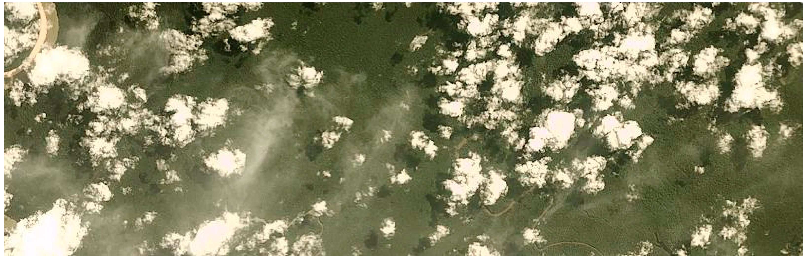
Figure 4 and
Figure 5 illustrates the sample images of cloudy and partly cloudy conditions.
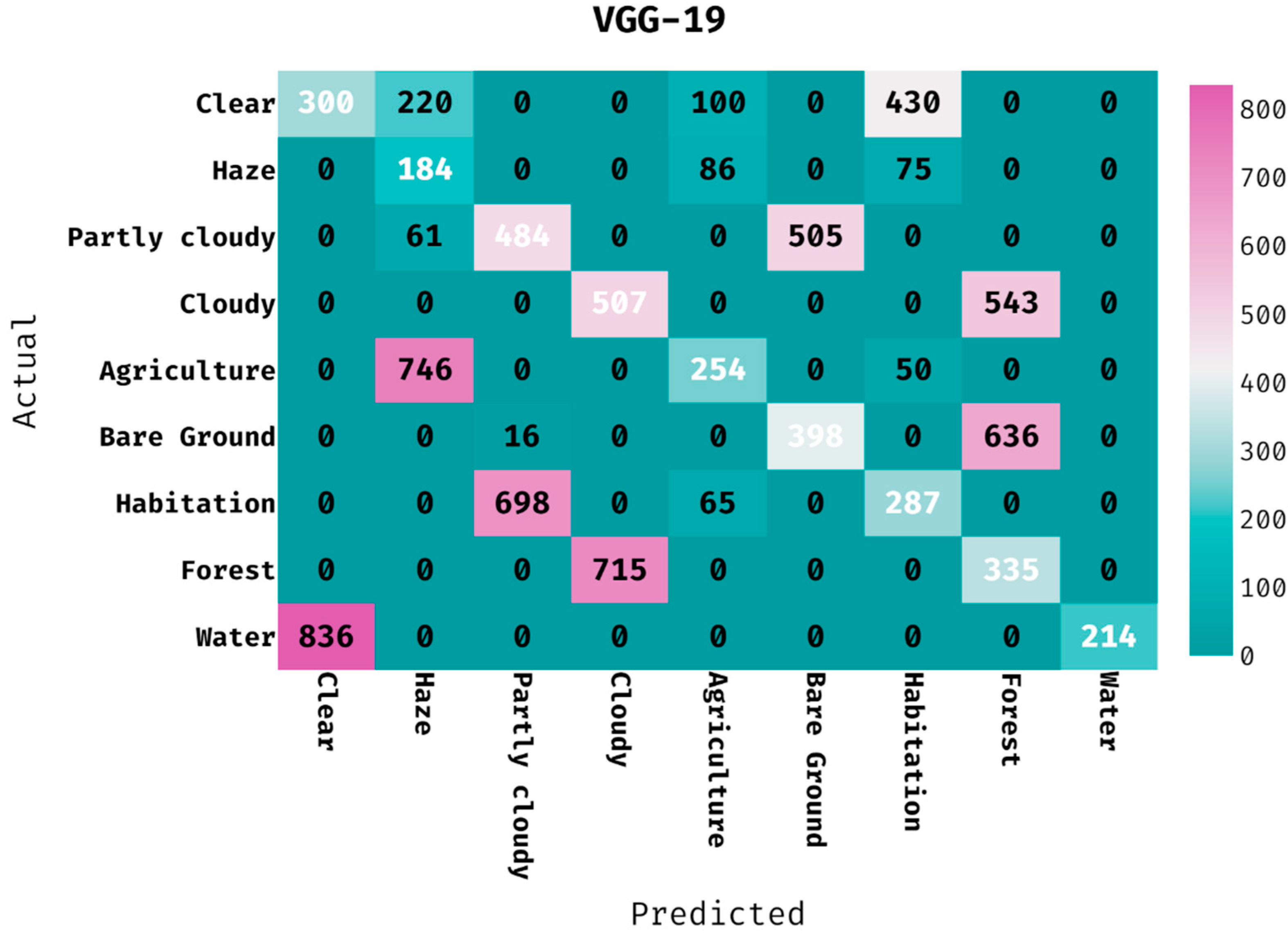
The confusion matrix generated by the VGG-19 model on land cover classification is given in
Figure 6. The figure has shown that the VGG-19 model has classified 300 images into Clear, 184 images into Haze, 484 images into Partly Cloudy, 507 images into Cloudy, 254 images into Agriculture, 398 images into Bare Ground, 287 images into Habitation, 335 images into Forest, and 214 images into Water.
Table 1 provides the classification results of the VGG-19 model on the applied dataset. The results demonstrated that the VGG-19 model has proficiently categorized the images into distinct classes. For instance, the VGG-19 model has classified the images into ‘clear’ class with the PPV of 0.264, hit rate of 0.286, accuracy of 0.819, F-measure of 0.275, and MCC of 0.171. In addition, the VGG-19 method has categorized the images into ‘partly cloudy’ class with the PPV of 0.404, hit rate of 0.461, accuracy of 0.854, F-measure of 0.431, and MCC of 0.348. Further, the VGG-19 approach has ordered the images into ‘agriculture’ class with the PPV of 0.503, hit rate of 0.242, accuracy of 0.880, F-measure of 0.327, and MCC of 0.292. Concurrently, the VGG-19 technique has classified the images into ‘habitation’ class with the PPV of 0.341, hit rate of 0.273, accuracy of 0.849, F-measure of 0.303, and MCC of 0.222. Eventually, the VGG-19 methodology has categorized the images into ‘water’ class with the PPV of 1.000, hit rate of 0.204, accuracy of 0.904, F-measure of 0.339, and MCC of 0.429.
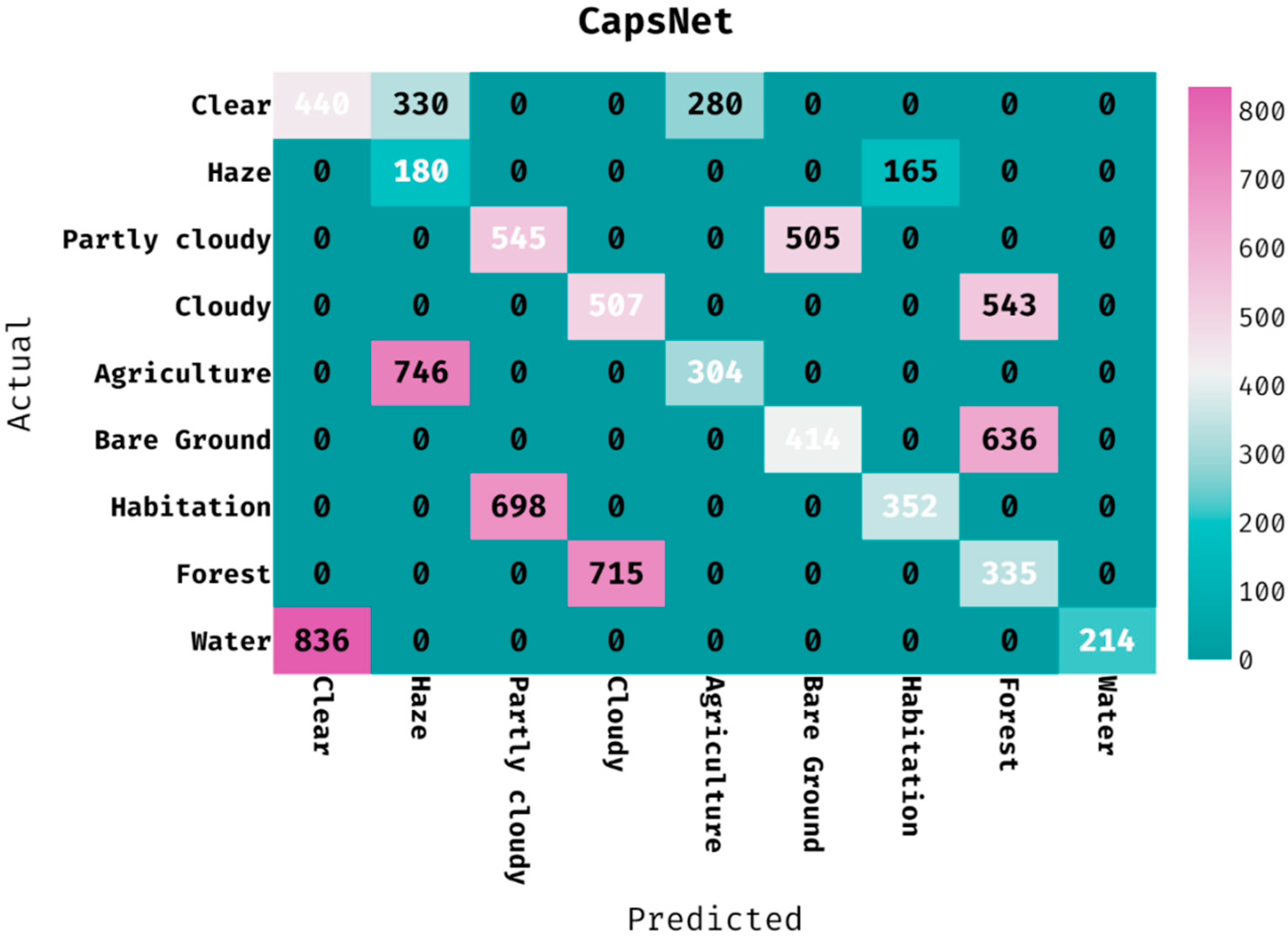
The confusion matrix generated by the CapsNet approach on the classification of land cover is provided in
Figure 7. The figure demonstrated that the CapsNet manner has classified 440 images into clear, 180 images into haze, 545 images into partly cloudy, 507 images into cloudy, 304 images into agriculture, 414 images into bare ground, 352 images into habitation, 335 images into forest, and 214 images into water.
Table 2 gives the classification outcomes of the CAPSNET manner on the applied dataset. The results outperformed that the CapsNet method has proficiently categorized the images into different classes. For instance, the CapsNet algorithm has ordered the images into ‘clear’ class with the PPV of 0.345, hit rate of 0.419, accuracy of 0.835, F-measure of 0.378, and MCC of 0.286. Additionally, the CapsNet technique has classified the image into ‘partly cloudy’ class with the PPV of 0.439, hit rate of 0.519, accuracy of 0.862, F-measure of 0.475, and MCC of 0.399. In the meantime, the CapsNet approach has categorized the images into ‘agriculture’ class with the PPV of 0.521, hit rate of 0.290, accuracy of 0.883, F-measure of 0.372, and MCC of 0.330. In line with, the CapsNet system has classified the image into ‘habitation’ class with the PPV of 0.681, hit rate of 0.335, accuracy of 0.901, F-measure of 0.449, and MCC of 0.433. At last, the CapsNet algorithm has ordered the images into ‘water’ class with the PPV of 1.000, hit rate of 0.204, accuracy of 0.904, F-measure of 0.339, and MCC of 0.429.
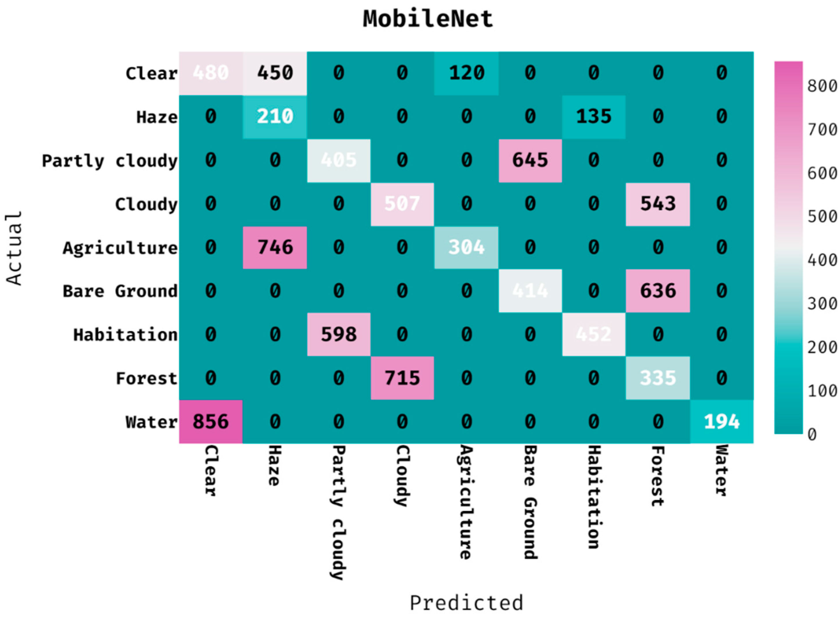
The confusion matrix produced by the MobileNet technique on the classification of land cover is provided in
Figure 8. The figure depicted that the MobileNet manner has classified 480 images into clear, 210 images into haze, 405 images into partly cloudy, 507 images into cloudy, 304 images into agriculture, 414 images into bare ground, 452 images into habitation, 335 images into forest, and 194 images into water.
Table 3 offers the classification outcomes of the MobileNet algorithm on the applied dataset. The results showcased that the MobileNet method has proficiently categorized the images into varying classes. For instance, the MobileNet approach has classified the images into ‘clear’ class with the PPV of 0.359, hit rate of 0.457, accuracy of 0.837, F-measure of 0.402, and MCC of 0.313. Moreover, the MobileNet method has categorized the images into ‘partly cloudy’ class with the PPV of 0.404, hit rate of 0.386, accuracy of 0.858, F-measure of 0.395, and MCC of 0.314. Meanwhile, the MobileNet algorithm has ordered the images into ‘agriculture’ class with the PPV of 0.717, hit rate of 0.290, accuracy of 0.901, F-measure of 0.413, and MCC of 0.415. Along with that, the MobileNet manner has categorized the images into ‘habitation’ class with the PPV of 0.770, hit rate of 0.431, accuracy of 0.916, F-measure of 0.552, and MCC of 0.536. Lastly, the MobileNet methodology has classified the image into ‘water’ class with the PPV of 1.000, hit rate of 0.185, accuracy of 0.902, F-measure of 0.312, and MCC of 0.408.
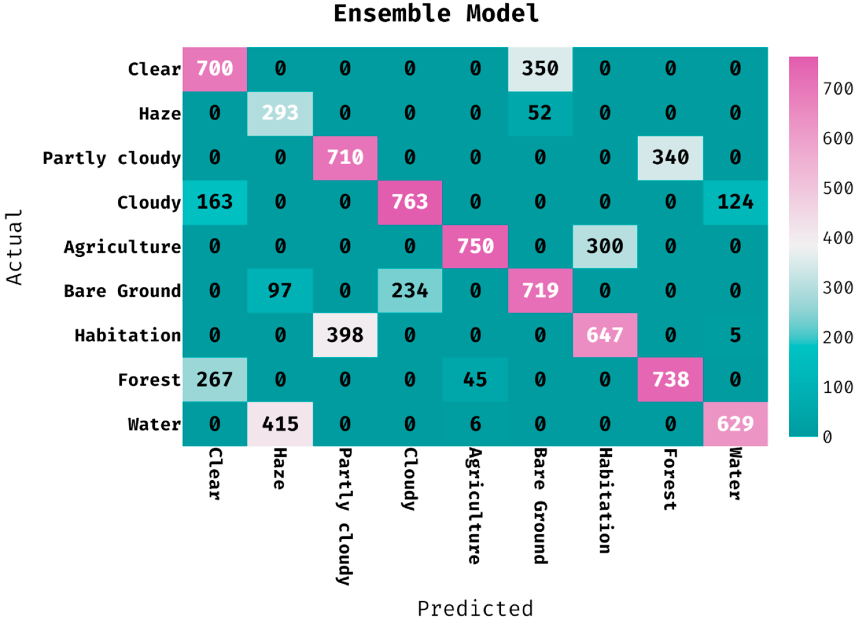
The confusion matrix created by the ensemble algorithm on the classification of land cover is provided in
Figure 9. The figure portrayed that the ensemble technique has classified 700 images into clear, 293 images into haze, 710 images into partly cloudy, 763 images into cloudy, 750 images into agriculture, 719 images into bare ground, 647 images into habitation, 738 images into forest, and 629 images into water.
Table 4 offers the classification outcomes of the ensemble technique on the applied dataset. The outcomes outperformed that the ensemble model has proficiently categorized the images into several classes. For instance, the ensemble system has ordered the images into ‘clear’ class with the PPV of 0.620, hit rate of 0.667, accuracy of 0.911, F-measure of 0.642, and MCC of 0.592. In addition, the ensemble algorithm has classified the image into ‘partly cloudy’ class with the PPV of 0.641, hit rate of 0.676, accuracy of 0.916, F-measure of 0.658, and MCC of 0.610. Further, the ensemble method has categorized the images into ‘agriculture’ class with the PPV of 0.936, hit rate of 0.714, accuracy of 0.960, F-measure of 0.810, and MCC of 0.797. Concurrently, the ensemble methodology has classified the image into ‘habitation’ class with the PPV of 0.683, hit rate of 0.616, accuracy of 0.920, F-measure of 0.648, and MCC of 0.604. Eventually, the ensemble technique has categorized the images into ‘water’ class with the PPV of 0.830, hit rate of 0.599, accuracy of 0.937, F-measure of 0.696, and MCC of 0.673.
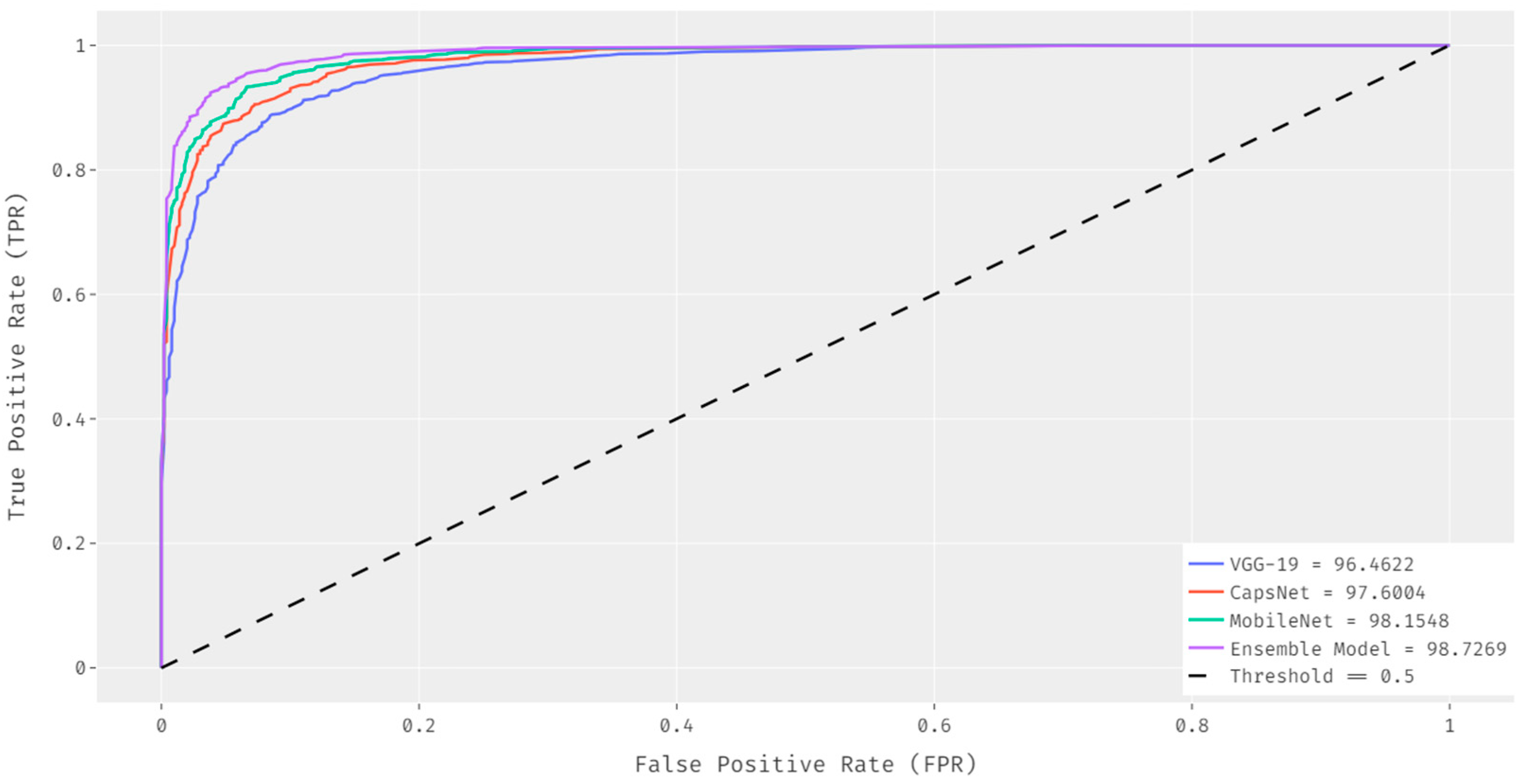
Figure 10 shows the comparative ROC analysis of the EDL-MMLCC technique with other DL models. The results demonstrated that the ensemble model has resulted to an increased ROC of 98.3854 whereas the VGG-19, CapsNet, and MobileNet techniques have attained a reduced ROC of 94.4794, 95.9203, and 97.7137 respectively.
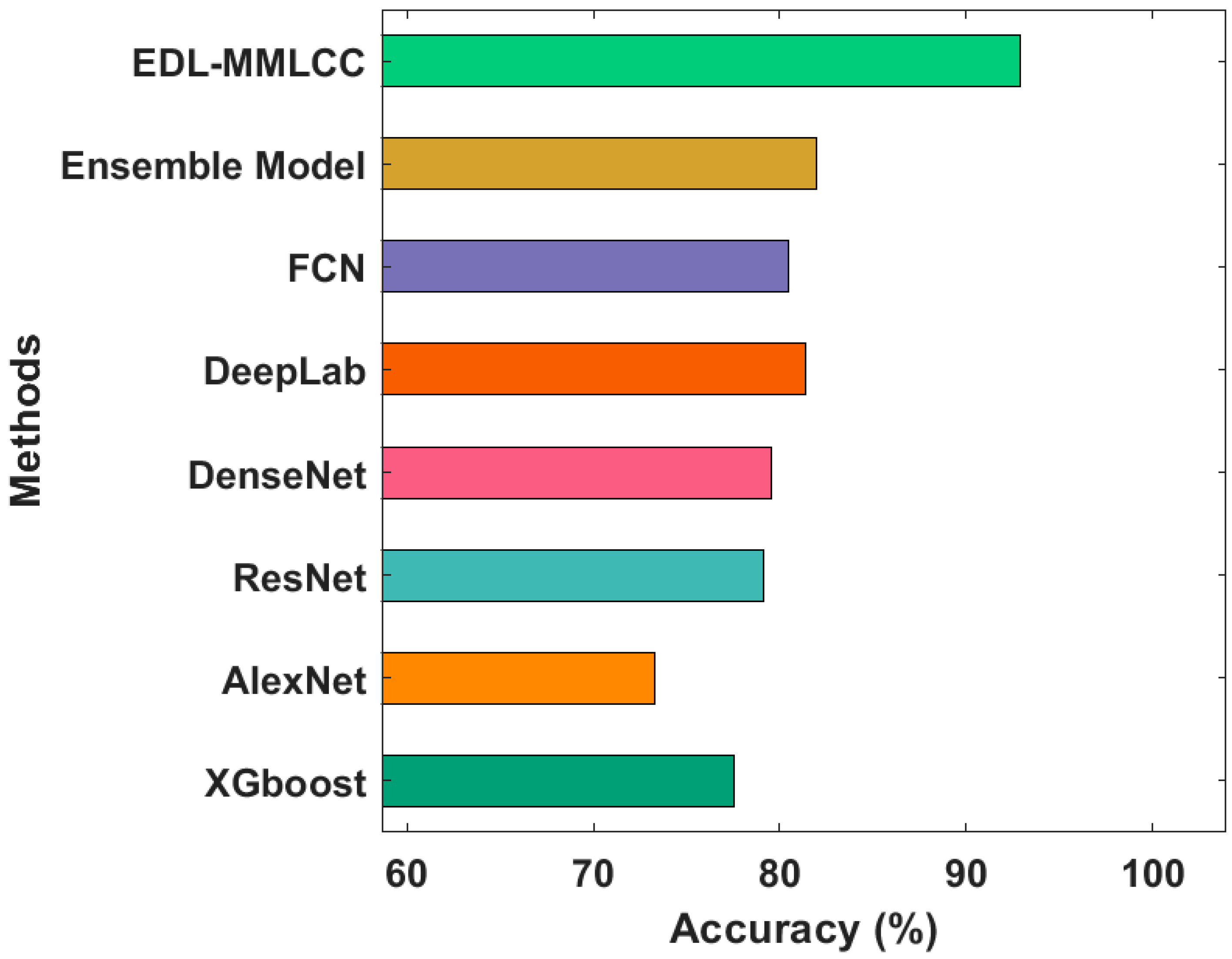
Finally, a brief comparative study of the EDL-MMLCC with existing techniques takes place in
Figure 11 [
26]. The results portrayed that the XGBoost and AlexNet techniques have resulted in lowering accuracy of 77.55% and 73.29% respectively. In addition, the ResNet and DenseNet models have obtained slightly improved outcomes with the accuracy of 79.13% and 79.55%, respectively. Eventually, the DeepLab and FCN techniques have accomplished near-optimal outcomes with an accuracy of 80.48%. Though the ensemble model has resulted in a competitive accuracy of 82%, the proposed EDL-MMLCC technique has accomplished superior performance with an accuracy of 92.90%. By looking into the above mentioned tables and figures, it can be evident that the EDL-MMLCC manner has resulted in an effective land cover classification tool using remote sensing images.


 ,
, 


