Semiclassical Approach to the Nonlocal Kinetic Model of Metal Vapor Active Media

Abstract

A semiclassical approach based on the WKB–Maslov method is developed for the kinetic ionization equation in dense plasma with approximations characteristic of metal vapor active media excited by a contracted discharge. We develop the technique for constructing the leading term of the semiclassical asymptotics of the Cauchy problem solution for the kinetic equation under the supposition of weak diffusion. In terms of the approach developed, the local cubic nonlinear term in the original kinetic equation is considered in a nonlocal form. This allows one to transform the nonlinear nonlocal kinetic equation to an associated linear partial differential equation with a given accuracy of the asymptotic parameter using the dynamical system of moments of the desired solution of the equation. The Cauchy problem solution for the nonlinear nonlocal kinetic equation can be obtained from the solution of the associated linear partial differential equation and some algebraic equations for the coefficients of the linear equation. Within the developed approach, the plasma relaxation in metal vapor active media is studied with asymptotic solutions expressed in terms of higher transcendental functions. The qualitative analysis of such the solutions is given.

1. Introduction

Studies of kinetics of metal vapor active media (MVAM) are motivated by their wide application in the development of laser systems. MVAM are used in technics due to their high optical gain in a narrow spectral range [1,2,3]. Nowadays, the most promising application of MVAM are the active optical systems (the so-called laser monitors) that allow one to visualize the processes blocked by the intense strong background light [4,5].

The active media on metal vapors are a mixture of a buffer gas (inert gas) and a gaseous metal, and the concentration of the buffer gas is 2–3 orders of magnitude higher than the concentration of metal vapors. Under the action of an electric discharge, the processes of ionization and recombination in such media occur mainly due to the reactions of electron impact. The inelastic collisions of neutral atoms with electrons are responsible for ionization, and triple recombination processes (triple collision of an ion with two electrons) are responsible for deionization. In MVAM, mainly metal atoms are ionized, and the buffer gas practically does not contribute to the concentration of the electron gas due to the much higher ionization energy. In a number of works (see, for example, [6,7,8,9,10]), active media were investigated, where neon acted as a buffer gas, and vapors of copper and its halides did as an active substance.

Note that a mixture of a buffer gas and metal vapors in this case is inside the gas discharge tube (GDT). However, under the condition of a strongly contracted pumping discharge of the active medium, the ions will be localized around the center of the GDT, and there will be no boundary conditions on the GDT walls in the mathematical problem statement. Here, we will consider just such a case when the ion concentration rapidly decreases with distance from the center of the GDT. The equation for the concentration of positive singly charged ions $n_i(\overrightarrow{x},t)$ of a metal for a constant gas temperature according to the law of mass action can be written as [11]

$$\begin{array}{c}{\partial }_t{n}_i(\overrightarrow{x},t)=D_a\left(t\right)\Delta n_i(\overrightarrow{x},t)+q_i(\overrightarrow{x},t)n_e(\overrightarrow{x},t)n_{neut}(\overrightarrow{x},t)-\\ -q_{tr}(\overrightarrow{x},t)n_i(\overrightarrow{x},t){\left(n_e(\overrightarrow{x},t)\right)}^2,\end{array}$$

(1)

where the space and time variables are denoted by $\overrightarrow{x}(\in {\mathbb{R}}^n)$ and $t(\in R^1)$, respectively, ${\partial }_t=\partial /\partial t$; $q_i(\overrightarrow{x},t)$ is rate constant of the electron impact ionization process, and $q_{tr}(\overrightarrow{x},t)$ is the rate constant of the triple recombination process. The ambipolar diffusion coefficient is $D_a\left(t\right)$; the concentration of neutral metal atoms is $n_{neut}(\overrightarrow{x},t)$, and $n_e(\overrightarrow{x},t)$ is the concentration of electrons. The dependence of the coefficients $q_i$, $q_{tr}$ and $D_a$ on $\overrightarrow{x}$ and t is due to their dependence on the electron temperature which can be substantially inhomogeneous in time and space. When the discharge energy is insufficient for the complete ionization of metal vapors, then only singly charged ions are produced in the plasma. Therefore, in view of the plasma quasineutrality, the concentration distribution of positive singly charged ions, $n_i(\overrightarrow{x},t)$, coincides with the concentration distribution of electrons, $n_e(\overrightarrow{x},t)$, i.e.,

$$\begin{array}{c}\hfill n_e(\overrightarrow{x},t)=n_i(\overrightarrow{x},t).\end{array}$$

(2)

The properties of active media that are useful for applications appear when the upper resonance energy level of metal atoms is effectively pumped. In such the conditions, the degree of ionization is small, i.e.,

$$\begin{array}{c}\hfill n_{neut}(\overrightarrow{x},t)\gg n_i(\overrightarrow{x},t),\end{array}$$

(3)

and $n_{neut}$ almost does not depend on $n_i$. In practice, $n_{neut}$ is at least one order greater than $n_i$ for MVAM. Under conditions (2), (3), the Equation (1) becomes closed and can be written as

$$\begin{array}{c}{\partial }_t{n}_i(\overrightarrow{x},t)=D_a\left(t\right)\Delta n_i(\overrightarrow{x},t)+a(\overrightarrow{x},t)n_i(\overrightarrow{x},t)-q_{tr}(\overrightarrow{x},t)n_i^3(\overrightarrow{x},t),\end{array}$$

(4)

where $a(\overrightarrow{x},t)=q_i(\overrightarrow{x},t)n_{neut}(\overrightarrow{x},t)$, $q_{tr}(\overrightarrow{x},t)$, and $D_a\left(t\right)$ are given functions. For $D_a=\mathrm{const}$, $a=\mathrm{const}$, $q_{tr}=\mathrm{const}$, the Equation (2) is termed the Newell–Whitehead equation [12,13]. The kinetic equation with a cubic nonlinearity of the form (4) has applications going beyond the plasma physics. For example, it can be treated as a dissipative part of the Gross–Pitaevskii equation with a phenomenological damping that describes the formation of vortices in Bose–Einstein condensates [14,15] or as a model equation for the imaginary-time method of constructing stationary solutions of the Gross–Pitaevskii equation [16,17,18].

We assume in (1) that diffusion and ionization/recombination processes occur at different scales in spatial coordinates. This approximation is applied when the electron temperature has a weak spatial inhomogeneity. The ambipolar diffusion coefficient $D_a\left(t\right)$ is assumed to be $D_a\left(t\right)=D_i(1+{\displaystyle \frac{T_e\left(t\right)}{T_g})}$, where $T_e\left(t\right)$ is the electron temperature, $T_g$ is the gas temperature, and the ion diffusion coefficient $D_i$ is independent of the spatial variables. The dependence of $q_i$ and $q_{tr}$ on the electron temperature is stronger than that of $D_a$. Therefore even a weak dependence of the electron temperature on the spatial variables can lead to a significant dependence of $q_i$ and $q_{tr}$ on $\overrightarrow{x}$. We do not take into account the dielectronic recombination process in the Equation (1) since it makes a significant contribution to the ion concentration only in a rarefied plasma with pressures much lower than those that are characteristic of the operation of MVAM. Additionally, we do not take into consideration the Penning ionization that is significant in MVAM where the buffer gas pressure under normal conditions is higher than one hundred torr, while it is only 20–30 torr in most present-day works.

The coefficients $q_i(\overrightarrow{x},t)$ and $q_{tr}(\overrightarrow{x},t)$ in Equation (1) mean the total rates of the corresponding processes including stepwise ionization and also recombination to the lower energy states of neutral atoms. This approximation allows one not to solve a system of a large number of equations where each equation describes a population of an individual energy level of neutral atoms. This approximation is widely used in describing the ionization in plasma, since direct experimental data usually give the values of the total ionization rates (see, e.g., [14]. The total rate of triple recombination is determined on the basis of the semiclassical approach described in the work of Gurevich and Pitaevskii [15].

Equation (1) plays an important role in the design of MVAM. The influence of the prepulse electron concentration on characteristics of active media on copper vapors was discussed in detail in [16,17]. In particular, solutions to the Equation (1) were required to construct a high-voltage high-frequency pumping circuit for exciting the active medium for laser monitors. The plasma itself has an active–inductive resistance character. In this case, the active component of the resistance prevails. This parameter significantly depends on time within the pump pulse period and it is a complex function of the temperature and electron concentration. Therefore, to match the pumping circuit with the load, models of the resistance of the active medium are used. These models include the electron concentration or, at least, its prepulse value (see, e.g., [18]). The main way of determining it is related to solutions of kinetic equations. The kinetic modeling of such active media began to develop in the 1980s–1990s (see, e.g., [11,19,20,21]). The approach for constructing a space-time kinetic model of active media on copper vapor was developed in [22,23,24] where the model equations were studied mainly numerically.

The aim of this work is to develop an analytical approach based on the WKB–Maslov theory of the semiclassical approximation [25,26,27] to study the kinetic equation of plasma ionization.

The method of semiclassical asymptotics was applied in [28,29,30] to a nonlocal generalization of the Fisher–Kolmogorov–Petrovskii–Piskunov equation known in the theory of biological populations, and also in [31,32,33] for the nonlocal Gross–Pitaevskii equation, which is widely used in the theory of Bose–Einstein condensates. The approach proposed here for the kinetic equation of plasma ionization essentially involves the results of [28,29,30].

The paper is structured as follows. In Section 2, we introduce basic notations and the problem setup. The class of semiclassically concentrated functions, where asymptotics are constructed, is presented. In Section 3, the dynamical system describing the evolution of moments of the unknown solution is deduced and it is considered within the framework of our approach. In Section 4, the family of associated linear equations is obtained. The leading term of an asymptotic solution to the original nonlinear kinetic equation is constructed from solutions of these equations according to the certain algebraic conditions. Section 5 illustrates a general approach with the specific example of the plasma relaxation problem. In Section 6, the concluding remarks are given.

2. Nonlocal Kinetic Equation and Semiclassical Approximation

To apply the method of semiclassical asymptotics in accordance with [30,32], we consider a nonlocal version of the kinetic Equation (1).

In the local Equation (1), triple recombination is described in terms of a contact interaction model. If we introduce into the model the dependence of the probability of the act of triple recombination on the mutual arrangement of the particles participating in it, then we obtain a nonlocal generalization of the Equation (1) of the form

$$\begin{array}{c}{\partial }_t{n}_i(\overrightarrow{x},t)=D_a\left(t\right)\Delta n_i(\overrightarrow{x},t)+q_i(\overrightarrow{x},t)n_{neut}(\overrightarrow{x},t)n_e(\overrightarrow{x},t)-\\ {\displaystyle -\varkappa ·n_i(\overrightarrow{x},t)\underset{{\mathbb{R}}^n\times {\mathbb{R}}^n}{\int }b(\overrightarrow{x},\overrightarrow{y},\overrightarrow{z},t)n_e(\overrightarrow{y},t)n_e(\overrightarrow{z},t)d\overrightarrow{y}d\overrightarrow{z}.}\end{array}$$

(5)

Here, the kernel $b(\overrightarrow{x},\overrightarrow{y},\overrightarrow{z},t)$ of the integral term has the meaning of the probability density of the capture by an ion at the point $\overrightarrow{x}$ of an electron at the point $\overrightarrow{y}$, and an electron at the point $\overrightarrow{z}$ with subsequent triple recombination. For convenience, we have explicitly identified the normalization nonlinearity parameter $\varkappa$.

The probability of triple recombination depends on the electron thermal velocity and on the mutual distance between the electrons and the ion. Therefore, in specific examples of the Equation (5), we will assume

$$\begin{array}{c}b(\overrightarrow{x},\overrightarrow{y},\overrightarrow{z},t)=\tilde{b}(\overrightarrow{x},\overrightarrow{x}-\overrightarrow{y},\overrightarrow{x}-\overrightarrow{z},t),\end{array}$$

(6)

where the dependence of $\tilde{b}(\overrightarrow{x},{\overrightarrow{r}}_1,{\overrightarrow{r}}_2,t)$ on $\overrightarrow{x}$ and t is caused by its dependence on the electron temperature.

Further, we denote $D_a\left(t\right)=D·{\tilde{D}}_a\left(t\right)$ in the Equation (5), where D plays the role of an small diffusion parameter in the proposed method of semiclassical asymptotics, and the function ${\tilde{D}}_a\left(t\right)$ is considered given. In accordance with (2)–(4), we set $n_e=n_i$ in the Equation (5), denote $n_i(\overrightarrow{x},t)=u(\overrightarrow{x},t)$, and the Equation (5) takes the form

$$\begin{array}{c}{\partial }_{t}u(\overrightarrow{x},t)=D{\tilde{D}}_a\left(t\right)\Delta u(\overrightarrow{x},t)+a(\overrightarrow{x},t)u(\overrightarrow{x},t)-\\ {\displaystyle -\varkappa u(\overrightarrow{x},t)\underset{{\mathbb{R}}^n\times {\mathbb{R}}^n}{\int }b(\overrightarrow{x},\overrightarrow{y},\overrightarrow{z},t)u(\overrightarrow{y},t)u(\overrightarrow{z},t)d\overrightarrow{y}d\overrightarrow{z},}\end{array}$$

(7)

where $a(\overrightarrow{x},t)$, $b(\overrightarrow{x},\overrightarrow{y},\overrightarrow{z},t)$ are considered to be a given infinitely smooth functions with respect to spatial variables at each point t that increase, as $|\overrightarrow{x}|\to \infty$, $|\overrightarrow{y}|\to \infty$, $|\overrightarrow{z}|\to \infty$, not faster than the polynomial.

We will seek solutions u of the Equation (7) in the class ${\mathcal{P}}_D^t$ of trajectory-concentrated functions (TCFs) depending on the parameter D [28,29,30,34]:

$${\displaystyle {\mathcal{P}}_D^t=\left\{\Phi :\Phi (\overrightarrow{x},t,D)=\phi \left(\frac{\Delta \overrightarrow{x}}{\sqrt{D}},t,D\right)exp\left[\frac{1}{D}S(t,D)\right]\right\}.}$$

(8)

Here, $\Phi (\overrightarrow{x},t,D)$ is a common element of the class, the real function $\phi (\overrightarrow{\xi },t,D)$ belongs to the Schwartz space $\mathbb{S}$ in variables $\overrightarrow{\xi }$, smoothly depends on t and regularly depends on $\sqrt{D}$ as $D\to 0$, $\Delta \overrightarrow{x}=\overrightarrow{x}-\overrightarrow{X}(t,D)$. The real smooth functions $\overrightarrow{X}(t,D)$ and $S(t,D)$, characterizing the class ${\mathcal{P}}_D^t$, regularly depend on $\sqrt{D}$ as $D\to 0$ and are to be determined when constructing a solution to the Equation (7).

The functions of the class ${\mathcal{P}}_D^t$ are concentrated, as $D\to 0$, in a neighborhood of a point moving in the coordinate space along a curve given by the equation $\overrightarrow{x}=\overrightarrow{X}(t,0)$.

In addition to $\Delta \overrightarrow{x}$, we introduce the following operators acting on functions of the class ${\mathcal{P}}_D^t$: $\widehat{\overrightarrow{p}}=D{\partial }_{\overrightarrow{x}}$, $\widehat{T}=D{\partial }_t+\langle \dot{\overrightarrow{X}}(t,D),\widehat{\overrightarrow{p}}\rangle -\dot{S}(t,D)$, and ${\widehat{\Delta }}_{\alpha ,\beta }(t,D)$, where $\langle ,\rangle$ means the scalar product of n–dimensional vectors; ${\partial }_{\overrightarrow{x}}$ is the gradient operator in Cartesian coordinates $\overrightarrow{x}$; the operator ${\widehat{\Delta }}_{\mu ,\nu }(t,D)$ is defined by its Weil symbol ${\Delta }_{\mu ,\nu }(\overrightarrow{p},\overrightarrow{x},t,D)={\overrightarrow{p}}^{\mu }\Delta {\overrightarrow{x}}^{\nu }$, $\overrightarrow{p}\in {\mathbb{R}}^n$ is the symbol of the operator $\widehat{\overrightarrow{p}}$; $\mu ,\nu \in {\mathbb{Z}}_{+}^n$ are multi-indices:

$$\begin{array}{cc}\hfill & \nu =({\nu }_1,{\nu }_2,\dots ,{\nu }_n),{\nu }_1,{\nu }_1,\dots ,{\nu }_n\in {\mathbb{Z}}_{+}^1,\hfill \\ \hfill & \left|\nu \right|={\nu }_1+{\nu }_2+\dots +{\nu }_n,\nu !={\nu }_1!{\nu }_2!\dots {\nu }_n!.\hfill \end{array}$$

(9)

For any vector $\overrightarrow{a}=(a_1,a_2,\dots ,a_n)\in {\mathbb{R}}^n$ we denote ${\overrightarrow{a}}^{\nu }=(a_1^{{\nu }_1},a_2^{{\nu }_2},\cdots ,a_n^{{\nu }_n})\in {\mathbb{R}}^n$.

One can directly verify the validity of the following asymptotic estimates for the operators and the functions from the class ${\mathcal{P}}_D^t$ [34,35]:

$$\begin{array}{cc}\hfill & {\displaystyle \frac{\Vert {\widehat{\Delta }}_{\mu ,\nu }(t,D)\Phi \Vert }{\Vert \Phi \Vert }=\mathrm{O}\left(D^{\left(\right|\mu |+|\nu \left|\right)/2}\right),\frac{\Vert \widehat{T}\Phi \Vert }{\Vert \Phi \Vert }=\mathrm{O}\left(D\right),\Phi \in {\mathcal{P}}_D^t,}\hfill \end{array}$$

(10)

where the norm $\Vert \dots \Vert$ is meant in the sense of the space $L_2$.

Formulas (10) can be considered as estimates of the operators acting on functions of the class ${\mathcal{P}}_D^t$:

$$\begin{array}{cc}\hfill & {\widehat{\Delta }}_{\mu ,\nu }(t,D)=\widehat{\mathrm{O}}\left(D^{\left(\right|\mu |+|\nu \left|\right)/2}\right),\widehat{T}=\widehat{\mathrm{O}}\left(D\right),\hfill \end{array}$$

(11)

and, in particular, $\Delta \overrightarrow{x}=\widehat{\mathrm{O}}\left(\sqrt{D}\right)$, $\widehat{\overrightarrow{p}}=\widehat{\mathrm{O}}\left(\sqrt{D}\right)$. Here, $\widehat{\mathrm{O}}\left(D^k\right)$, $k\ge 0$, means an operator $\widehat{F}$ such that $\Vert \widehat{F}\varphi \Vert /\Vert \varphi \Vert =\mathrm{O}\left(D^k\right)$, $\varphi \in {\mathcal{P}}_D^t$.

In the asymptotic estimates, the leading term gives more insight into the solution of the problem. Therefore, in this work, we focus on constructing the leading terms of asymptotic solutions of the kinetic Equation (7).

3. The Einstein–Ehrenfest System of the Second Order

The semiclassical approach developed in [30,31,32] can be applied to Equation (7) when the following moments exist for its solution $u(\overrightarrow{x},t,D)\in {\mathcal{P}}_D^t$:

$$\begin{array}{cc}\hfill & {\displaystyle {\sigma }_u(t,D)=\underset{{\mathbb{R}}^n}{\int }u(\overrightarrow{x},t,D)d\overrightarrow{x},{\overrightarrow{x}}_u(t,D)=\frac{1}{{\sigma }_u(t,D)}\underset{{\mathbb{R}}^n}{\int }\overrightarrow{x}u(\overrightarrow{x},t,D)d\overrightarrow{x}}\hfill \end{array}$$

(12)

$$\begin{array}{cc}\hfill & {\displaystyle {\alpha }_u^{\nu }(t,D)=\frac{1}{{\sigma }_u(t,D)}\underset{{\mathbb{R}}^n}{\int }\Delta \overrightarrow{x}{}^{\nu }u(\overrightarrow{x},t,D)d\overrightarrow{x},\nu =({\nu }_1,{\nu }_2,\dots ,{\nu }_n)\in {\mathbb{Z}}_{+}^n,\left|\nu \right|\in {\mathbb{Z}}_{+}^1.}\hfill \end{array}$$

(13)

Here, the zeroth-order moment ${\sigma }_u(t,D)$ has the meaning of the number of ions in the plasma at time t.

We choose the vector $\overrightarrow{X}(t,D)$ characterizing the class ${\mathcal{P}}_D^t$ to be equal to the first normalized moment

$$\begin{array}{c}\hfill \overrightarrow{X}(t,D)={\overrightarrow{x}}_u(t,D).\end{array}$$

(14)

Then, ${\alpha }_u^{\nu }(t,D)=0$ for $\left|\nu \right|=1$.

We also limit our consideration to solutions $u(\overrightarrow{x},t,D)$ of (7) with ${\sigma }_u(t,D)=\mathrm{O}\left(1\right)$. Otherwise, the nonlinear term would be infinitely large compared to the linear term as $D\to 0$, i.e., the rate of triple recombination would dominate over the ionization rate at each t. In (5), the $\varkappa$ is defined so that the ionization processes compete with the triple recombination that is the most interesting case from a physical point of view.

Then from (10) we have

$$\begin{array}{cc}\hfill & {\overrightarrow{x}}_u(t,D)=\mathrm{O}\left(1\right),{\alpha }_u^{\nu }(t,D)=\mathrm{O}\left(D^{\left|\nu \right|/2}\right).\hfill \end{array}$$

(15)

For constructing the leading term of the semiclassical asymptotic solution to Equation (7), we consider a set of moments of the form (13), including ${\sigma }_u(t,D)$, ${\overrightarrow{x}}_u(t,D)$, and the second-order moments ${\alpha }_u^{\nu }(t,D)$, $\left|\nu \right|=2$, which can be represented in the form of a n–dimensional symmetric matrix

$$\begin{array}{cc}\hfill & {\alpha }_u^{\left(2\right)}(t,D)=\left({\alpha }_{u,ij}^{\left(2\right)}(t,D)\right),\hfill \end{array}$$

(16)

where ${\displaystyle {\alpha }_{u,ij}^{\left(2\right)}(t,D)=\frac{1}{{\sigma }_u(t,D)}\underset{{\mathbb{R}}^n}{\int }\Delta x_i\Delta x_{j}u(\overrightarrow{x},t,D)d\overrightarrow{x}}$, and $i,j=1,2,\dots ,n$.

For simplicity of notation, we introduce an aggregate vector of the considered moments

$$\begin{array}{cc}\hfill & {\Theta }_u(t,D)=\left({\sigma }_u(t,D),{\overrightarrow{x}}_u(t,D),{\alpha }_u^{\left(2\right)}(t,D)\right).\hfill \end{array}$$

(17)

In what follows, we will omit the function arguments, including the asymptotic parameter D, if this does not lead to a misunderstanding.

Let us obtain the dynamical system describing evolution of the moments (17). To do this, we represent the functions $a(\overrightarrow{x},t)$ and $b(\overrightarrow{x},\overrightarrow{y},\overrightarrow{z},t)$ in Equation (7) as the second-order Taylor series expansions about the point $\overrightarrow{X}(t,D)$. Using matrix notations, we can write

$$\begin{array}{cc}\hfill & a(\overrightarrow{x},t)=a(\overrightarrow{X},t)+a_x\Delta \overrightarrow{x}+\frac{1}{2}\Delta {\overrightarrow{x}}^T{a}_{xx}\Delta \overrightarrow{x}+\dots \left(\mathrm{h}\mathrm{i}\mathrm{g}\mathrm{h}\mathrm{e}\mathrm{r} \mathrm{o}\mathrm{r}\mathrm{d}\mathrm{e}\mathrm{r} \mathrm{t}\mathrm{e}\mathrm{r}\mathrm{m}\mathrm{s}\right),\hfill \end{array}$$

(18)

$$\begin{array}{cc}\hfill & b(\overrightarrow{x},\overrightarrow{y},\overrightarrow{z},t)=b(\overrightarrow{X},\overrightarrow{X},\overrightarrow{X},t)+b_x\Delta \overrightarrow{x}+b_y\Delta \overrightarrow{y}+b_z\Delta \overrightarrow{z}+\frac{1}{2}(\Delta {\overrightarrow{x}}^T{b}_{xx}\Delta \overrightarrow{x}+\hfill \\ \hfill & +\Delta {\overrightarrow{x}}^T{b}_{xy}\Delta \overrightarrow{y}+\Delta {\overrightarrow{y}}^T{b}_{yx}\Delta \overrightarrow{x}+\Delta {\overrightarrow{x}}^T{b}_{xz}\Delta \overrightarrow{z}+\Delta {\overrightarrow{z}}^T{b}_{zx}\Delta \overrightarrow{x}+\Delta {\overrightarrow{y}}^T{b}_{yy}\Delta \overrightarrow{y}+\hfill \\ \hfill & \Delta {\overrightarrow{y}}^T{b}_{yz}\Delta \overrightarrow{z}+\Delta {\overrightarrow{z}}^T{b}_{zy}\Delta \overrightarrow{y}+\Delta {\overrightarrow{z}}^T{b}_{zz}\Delta \overrightarrow{z})+\dots \left(\mathrm{h}\mathrm{i}\mathrm{g}\mathrm{h}\mathrm{e}\mathrm{r} \mathrm{o}\mathrm{r}\mathrm{d}\mathrm{e}\mathrm{r} \mathrm{t}\mathrm{e}\mathrm{r}\mathrm{m}\mathrm{s}\right).\hfill \end{array}$$

(19)

Here, $\Delta \overrightarrow{x}=\overrightarrow{x}-\overrightarrow{X}\left(t\right)$, $\Delta \overrightarrow{y}=\overrightarrow{y}-\overrightarrow{X}\left(t\right)$, $\Delta \overrightarrow{z}=\overrightarrow{z}-\overrightarrow{X}\left(t\right)$ are column vectors, the transposition is indicated by T; $a_x$, $b_x$, $b_y$, $b_z$ are row vectors, ${\displaystyle a_x=\left(\frac{\partial a}{\partial x_i}{|}_{\overrightarrow{x}=\overrightarrow{X}\left(t\right)}\right)}$, ${\displaystyle b_x=\left(\frac{\partial b}{\partial x_i}{|}_{\overrightarrow{x}=\overrightarrow{X}\left(t\right),\overrightarrow{y}=\overrightarrow{X}\left(t\right),\overrightarrow{z}=\overrightarrow{X}\left(t\right)}\right)}$, and the same for $b_y$ and $b_z$; $a_{xx}$, $b_{xx}$, $b_{yy}$, $b_{zz}$, $b_{xy}=b_{yx}$, $b_{xz}=b_{zx}$, $b_{zy}=b_{yz}$ are n-dimensional matrices of the form ${\displaystyle a_{xx}=\left(\frac{{\partial }^{2}a}{\partial x_i\partial x_j}{|}_{\overrightarrow{x}=\overrightarrow{X}\left(t\right)}\right)}$, ${\displaystyle b_{xx}=\left(\frac{{\partial }^{2}b}{\partial x_i\partial x_j}{|}_{\overrightarrow{x}=\overrightarrow{X}\left(t\right),\overrightarrow{y}=\overrightarrow{X}\left(t\right),\overrightarrow{z}=\overrightarrow{X}\left(t\right)}\right)}$, ${\displaystyle b_{xy}=\left(\frac{{\partial }^{2}b}{\partial x_i\partial y_j}{|}_{\overrightarrow{x}=\overrightarrow{X}\left(t\right),\overrightarrow{y}=\overrightarrow{X}\left(t\right),\overrightarrow{z}=\overrightarrow{X}\left(t\right)}\right)}$, and the same for $b_{yy}$, $b_{zz}$, $b_{xz}=b_{zx}$, $b_{zy}=b_{yz}$.

We also consider a particular expansion

$$\begin{array}{cc}\hfill & b(\overrightarrow{x},\overrightarrow{y},\overrightarrow{z},t)=b(\overrightarrow{x},\overrightarrow{X},\overrightarrow{X},t)+b_y\left(\overrightarrow{x}\right)\Delta \overrightarrow{y}+b_z\left(\overrightarrow{x}\right)\Delta \overrightarrow{z}+\frac{1}{2}(\Delta {\overrightarrow{y}}^T{b}_{yy}\left(\overrightarrow{x}\right)\Delta \overrightarrow{y}+\hfill \\ \hfill & \Delta {\overrightarrow{y}}^T{b}_{yz}\left(\overrightarrow{x}\right)\Delta \overrightarrow{z}+\Delta {\overrightarrow{z}}^T{b}_{zy}\left(\overrightarrow{x}\right)\Delta \overrightarrow{y}+\Delta {\overrightarrow{z}}^T{b}_{zz}\left(\overrightarrow{x}\right)\Delta \overrightarrow{z})+\dots \left(\mathrm{h}\mathrm{i}\mathrm{g}\mathrm{h}\mathrm{e}\mathrm{r} \mathrm{o}\mathrm{r}\mathrm{d}\mathrm{e}\mathrm{r} \mathrm{t}\mathrm{e}\mathrm{r}\mathrm{m}\mathrm{s}\right),\hfill \end{array}$$

(20)

where $b_y\left(\overrightarrow{x}\right)=$$b_y(\overrightarrow{x},\overrightarrow{X},\overrightarrow{X})$= ${\displaystyle \left(\frac{\partial b}{\partial y_i}{|}_{\overrightarrow{y}=\overrightarrow{X}\left(t\right),\overrightarrow{z}=\overrightarrow{X}\left(t\right)}\right)}$ and the same for $b_z\left(\overrightarrow{x}\right)$; $b_{yy}\left(\overrightarrow{x}\right)=$$b_{yy}(\overrightarrow{x},\overrightarrow{X},\overrightarrow{X})$= ${\displaystyle \left(\frac{{\partial }^{2}b}{\partial y_i\partial y_j}{|}_{\overrightarrow{y}=\overrightarrow{X}\left(t\right),\overrightarrow{z}=\overrightarrow{X}\left(t\right)}\right)}$, and the same for $b_{yz}\left(\overrightarrow{x}\right)=b_{zy}\left(\overrightarrow{x}\right)$, and $b_{zz}\left(\overrightarrow{x}\right)$.

To derive a dynamical system for moments (17), we differentiate the moments (17) with respect to time and substitute the derivative ${\partial }_{t}u$ from Equation (7). Taking into account expansions (18) and (19), and keeping the expansion terms no higher than the second order, we arrive at the equations

$$\begin{array}{cc}\hfill & {\displaystyle {\dot{\sigma }}_u={\sigma }_u\left(a(\overrightarrow{X},t)+\frac{1}{2}\mathrm{Sp}\left[a_{xx}{\alpha }_u^{\left(2\right)}\right]\right)-\varkappa {\sigma }_u^3(b(\overrightarrow{X},\overrightarrow{X},\overrightarrow{X},t)+}\hfill \\ \hfill & {\displaystyle +\frac{1}{2}\mathrm{Sp}\left[(b_{xx}+b_{yy}+b_{zz}){\alpha }_u^{\left(2\right)}\right]),}\hfill \end{array}$$

(21)

$$\begin{array}{cc}\hfill & {\dot{\overrightarrow{x}}}_u=\left(a_x-\varkappa {\sigma }_u^2{b}_x\right){\alpha }_u^{\left(2\right)},\hfill \end{array}$$

(22)

$$\begin{array}{cc}\hfill & {\dot{\alpha }}_u^{\left(2\right)}=2D{\tilde{D}}_a\left(t\right){\mathbb{I}}_{n\times n}.\hfill \end{array}$$

(23)

Here, dot denotes the time derivative (e.g., ${\dot{\sigma }}_u=d{\sigma }_u/dt$), $a_{xx}{\alpha }_u^{\left(2\right)}$ means matrix product, and ${\mathbb{I}}_{n\times n}$ is the identity matrix of size n, $\overrightarrow{X}={\overrightarrow{x}}_u(t,D)$ according to (14).

We can also rewrite Equations (21)–(23) more succinctly using the aggregate vector (17) as

$$\begin{array}{cc}\hfill & {\dot{\Theta }}_u(t,D)=\Gamma ({\Theta }_u(t,D),t,D),\hfill \end{array}$$

(24)

where

$$\begin{array}{cc}\hfill & \Gamma ({\Theta }_u(t,D),t,D)=\left(f({\Theta }_u(t,D),t,D),g({\Theta }_u(t,D),t,D),h({\Theta }_u(t,D),t,D)\right),\hfill \end{array}$$

(25)

consists of the functions f, g, h corresponding to ${\dot{\sigma }}_u$, ${\dot{\overrightarrow{x}}}_u$, and ${\dot{\alpha }}_u^{\left(2\right)}$, the form of which is obvious from (21)–(23), respectively.

Consider now a system of ordinary differential equations (ODEs)

$$\begin{array}{cc}\hfill & \dot{\Theta }\left(t\right)=\Gamma (\Theta \left(t\right),t,D)\hfill \end{array}$$

(26)

for an aggregate vector

$$\begin{array}{cc}\hfill & \Theta \left(t\right)=\left(\sigma \left(t\right),\overrightarrow{x}\left(t\right),{\alpha }^{\left(2\right)}\left(t\right)\right).\hfill \end{array}$$

(27)

Here, $\Gamma (\Theta (t),t,D)$ is taken from (25); real variable $\sigma \in {\mathbb{R}}^1$, real vector $\overrightarrow{x}\in {\mathbb{R}}^n$, and real symmetric matrix ${\alpha }^{\left(2\right)}=\left({\alpha }_{ij}^{\left(2\right)}\right)$ are the dependent variables.

Further in consideration of the system (26), we follow the papers [28,29,30].

According to [28,29,30], we call Equations (31) the Einstein–Ehrenfest (EE) system of the second order for the kinetic Equation (7). The second order of the EE system means the presence of ${\alpha }^{\left(2\right)}$ in (27).

Note that the Cauchy problem for the EE system (26) is known to have a unique solution under some conditions on the coefficients of the system, which are assumed to be satisfied.

Let Equation (7) have a solution $u(\overrightarrow{x},t,D)$ belonging to the class ${\mathcal{P}}_D^t$ given by (8) with the initial function

$$\begin{array}{cc}\hfill & u(\overrightarrow{x},t,D){|}_{t=0}=\phi (\overrightarrow{x},D),\hfill \end{array}$$

(28)

where the function $\phi (\overrightarrow{x},D)$ belongs to the class ${\mathcal{P}}_D^0$ of trajectory-concentrated functions (8) for $t=0$, ${\mathcal{P}}_D^0={\mathcal{P}}_D^t{|}_{t=0}$. Then, we can set the initial conditions for the the EE system (26) as

$$\begin{array}{cc}\hfill & {\Theta \left(t\right)|}_{t=0}={\mathfrak{g}}_{\phi }=\left({\sigma }_{\phi },{\overrightarrow{x}}_{\phi },{\alpha }_{\phi }^{\left(2\right)}\right),\hfill \end{array}$$

(29)

where

$$\begin{array}{cc}\hfill & {\displaystyle {\sigma |}_{t=0}={\sigma }_{\phi }=\underset{{\mathbb{R}}^n}{\int }\phi (\overrightarrow{x},D)d\overrightarrow{x},\overrightarrow{x}{|}_{t=0}={\overrightarrow{x}}_{\phi }=\frac{1}{{\sigma }_{\phi }}\underset{{\mathbb{R}}^n}{\int }\overrightarrow{x}\phi (\overrightarrow{x},D)d\overrightarrow{x},}\hfill \\ \hfill & {\displaystyle {\alpha }_{ij}^{\left(2\right)}{|}_{t=0}={\alpha }_{\phi ,ij}^{\left(2\right)}=\frac{1}{{\sigma }_{\phi }}\underset{{\mathbb{R}}^n}{\int }(x_i-x_{\phi ,i})(x_j-x_{\phi ,j})\phi (\overrightarrow{x},D)d\overrightarrow{x}.}\hfill \end{array}$$

(30)

We write the solution of the Cauchy problem for the EE system (26) with the initial conditions (29), (30) in the form

$$\begin{array}{c}\hfill {\mathfrak{g}}_{\phi }\left(t\right)=\left({\sigma }_{\phi }\left(t\right),{\overrightarrow{x}}_{\phi }\left(t\right),{\alpha }_{\phi }^{\left(2\right)}\left(t\right)\right),\end{array}$$

(31)

and

$$\mathfrak{g}(t,\mathbf{C})=\left(\sigma (t,\mathbf{C}),\overrightarrow{x}(t,\mathbf{C}),{\alpha }^{\left(2\right)}(t,\mathbf{C})\right)$$

(32)

is the general solution of the EE system (26), where $\mathbf{C}$ is a set of arbitrary integration constants. We omit the argument D in ${\sigma }_{\phi }\left(t\right)$, ${\overrightarrow{x}}_{\phi }\left(t\right)$, and ${\alpha }_{\phi }^{\left(2\right)}\left(t\right)$ for brevity.

Denote by ${\mathbf{C}}_{\phi }$ the solution of the following algebraic equation involving arbitrary integration constants $\mathbf{C}$ as unknowns:

$$\mathfrak{g}(0,\mathbf{C})={\mathfrak{g}}_{\phi },$$

(33)

i.e., $\mathfrak{g}(0,{\mathbf{C}}_{\phi })={\mathfrak{g}}_{\phi }$.

We consider the solution of Equation (33) in specific examples, leaving aside the general algebraic problem of solvability of this equation. Note also that ${\mathbf{C}}_{\phi }$ is a vector functional of $\phi$.

From the uniqueness of the solution of the Cauchy problem (26), (27), in view of (29), (30) and the condition (33), we have [28,30]

$$\mathfrak{g}(t,{\mathbf{C}}_{\phi })={\mathfrak{g}}_{\phi }\left(t\right).$$

(34)

On the other hand, we can consider the aggregate vector of moments ${\Theta }_u(t,D)$ (17) being determined by the solution $u(\overrightarrow{x},t,D)$ of Equation (7) with the initial condition (28). For uniformity, we denote it by

$$\begin{array}{c}\hfill {\mathfrak{g}}_u\left(t\right)=\left({\sigma }_u\left(t\right),{\overrightarrow{x}}_u\left(t\right),{\alpha }_u^{\left(2\right)}\left(t\right)\right).\end{array}$$

(35)

Since we consider the EE system of the second order, then $u(\overrightarrow{x},t,D)$ should be a leading term of the semiclassical asymptotic to Equation (7) accurate to $\mathrm{O}\left(D^{3/2}\right)$, and the subsequent analysis is carried out with this accuracy.

It can be seen that ${\mathfrak{g}}_u\left(t\right)$ satisfies the EE system (26) and the initial condition (29)

$$\begin{array}{c}\hfill {\mathfrak{g}}_u\left(0\right)={\mathfrak{g}}_{\phi }.\end{array}$$

(36)

Then we have

$$\begin{array}{c}\hfill {\mathfrak{g}}_u\left(t\right)={\mathfrak{g}}_{\phi }\left(t\right).\end{array}$$

(37)

In conclusion of this section, we defines values ${\mathbf{C}}_u\left(t\right)$ from the algebraic condition (33), but taken for any instant t:

$$\mathfrak{g}(t,{\mathbf{C}}_u\left(t\right))={\mathfrak{g}}_{\phi }\left(t\right).$$

(38)

From (38), (37), and (34), we find that ${\mathbf{C}}_u\left(t\right)={\mathbf{C}}_{\phi }$, i.e., the functionals ${\mathbf{C}}_u\left(t\right)$ can be considered as approximate integrals for the Equation (7) in the class (8) accurate to $\mathrm{O}\left(D^{3/2}\right)$.

4. Auxiliary Linear Problem and the Cauchy Problem

For constructing the leading term of the semiclassical asymptotic solution in the class (8), we first substitute the expansion (20) into the Equation (7). In view of the estimates (10) and formulae for the moments (12), (13), (16), we write

$$\begin{array}{c}\{-{\partial }_t+D{\tilde{D}}_a\left(t\right)\Delta +a(\overrightarrow{x},t)-\varkappa {\sigma }_u^2\left(t\right)(b(\overrightarrow{x},\overrightarrow{X}\left(t\right),\overrightarrow{X}\left(t\right),t)+\\ {\displaystyle +\frac{1}{2}\mathrm{Sp}\left[\left(b_{yy}(\overrightarrow{x},\overrightarrow{X},\overrightarrow{X},t)+b_{zz}(\overrightarrow{x},\overrightarrow{X},\overrightarrow{X},t)\right){\alpha }_u^{\left(2\right)}\left(t\right)\right]\left)\right\}u(\overrightarrow{x},t)=\mathrm{O}\left(D^{3/2}\right).}\end{array}$$

(39)

Here, the evolution of the moments ${\sigma }_u\left(t\right)$, $\overrightarrow{X}={\overrightarrow{x}}_u(t,D)$, and ${\alpha }_u^{\left(2\right)}\left(t\right)$ is governed by the dynamical system of the second order (21)–(23) or (24), (25) with the initial condition (29) when the initial condition (28) holds.

Next, we replace the moments (35) in the Equation (39) with the general solution of EE systems of the second order of the form (26), (27) given by (32) and go over the next linear equation parametrized by the arbitrary integration constants $\mathbf{C}$:

$$\begin{array}{c}\hfill \widehat{L}(\overrightarrow{x},t,\mathbf{C})v(\overrightarrow{x},t)=0,\end{array}$$

(40)

where

$$\begin{array}{cc}\hfill & \widehat{L}(\overrightarrow{x},t,\mathbf{C})=-{\partial }_t+D{\tilde{D}}_a\left(t\right)\Delta +a(\overrightarrow{x},t)-\varkappa {\sigma }^2(t,\mathbf{C})(b\left(\overrightarrow{x},\overrightarrow{x}(t,\mathbf{C}),\overrightarrow{x}(t,\mathbf{C})\right)+\hfill \\ \hfill & +\frac{1}{2}\mathrm{Sp}\left[\left(b_{yy}(\overrightarrow{x},\overrightarrow{x}(t,\mathbf{C}),\overrightarrow{x}(t,\mathbf{C}))+b_{zz}(\overrightarrow{x},\overrightarrow{x}(t,\mathbf{C}),\overrightarrow{x}(t,\mathbf{C}))\right){\alpha }^{\left(2\right)}(t,\mathbf{C})\right]).\hfill \end{array}$$

(41)

Here, $b_{yy}(\overrightarrow{x},\overrightarrow{x}(t,\mathbf{C}),\overrightarrow{x}(t,\mathbf{C}))=$ ${\displaystyle \left(\frac{{\partial }^{2}b}{\partial y_i\partial y_j}{|}_{\overrightarrow{y}=\overrightarrow{x}(t,\mathbf{C}),\overrightarrow{z}=\overrightarrow{x}(t,\mathbf{C})}\right)}$, and the same for $b_{zz}$.

By analogy, we can construct the following linear equation from (7) with the use of expansions (18) and (19):

$$\begin{array}{c}\hfill \widehat{\mathcal{L}}(\overrightarrow{x},t,\mathbf{C})v(\overrightarrow{x},t)=0,\end{array}$$

(42)

where

$$\begin{array}{cc}\hfill & {\displaystyle \widehat{\mathcal{L}}(\overrightarrow{x},t,\mathbf{C})=-{\partial }_t+D{\tilde{D}}_a\left(t\right)\Delta +L(t,\mathbf{C})+L_x(t,\mathbf{C})\Delta \overrightarrow{x}+\frac{1}{2}\Delta {\overrightarrow{x}}^T{L}_{xx}(t,\mathbf{C})\Delta \overrightarrow{x},}\hfill \end{array}$$

(43)

and

$$\begin{array}{cc}\hfill & L(t,\mathbf{C})=a(\overrightarrow{x}(t,\mathbf{C}),t)-\varkappa {\sigma }^2(t,\mathbf{C})(b\left(\overrightarrow{x}(t,\mathbf{C}),\overrightarrow{x}(t,\mathbf{C}),\overrightarrow{x}(t,\mathbf{C})\right)+\hfill \\ \hfill & +\frac{1}{2}\mathrm{Sp}\left[\left(b_{yy}(\overrightarrow{x}(t,\mathbf{C}),\overrightarrow{x}(t,\mathbf{C}),\overrightarrow{x}(t,\mathbf{C}))+b_{zz}(\overrightarrow{x}(t,\mathbf{C}),\overrightarrow{x}(t,\mathbf{C}),\overrightarrow{x}(t,\mathbf{C}))\right){\alpha }^{\left(2\right)}(t,\mathbf{C})\right]),\hfill \\ \hfill & L_x(t,\mathbf{C})=a_x(\overrightarrow{x}(t,\mathbf{C}),t)-\varkappa {\sigma }^2(t,\mathbf{C})b_x\left(\overrightarrow{x}(t,\mathbf{C}),\overrightarrow{x}(t,\mathbf{C}),\overrightarrow{x}(t,\mathbf{C})\right),\hfill \\ \hfill & L_{xx}(t,\mathbf{C})=a_{xx}(\overrightarrow{x}(t,\mathbf{C}),t)-\varkappa {\sigma }^2(t,\mathbf{C})b_{xx}\left(\overrightarrow{x}(t,\mathbf{C}),\overrightarrow{x}(t,\mathbf{C}),\overrightarrow{x}(t,\mathbf{C})\right).\hfill \end{array}$$

(44)

Note that in view of estimates (10) and (11), we can see that

$$\begin{array}{cc}\hfill & \widehat{L}(\overrightarrow{x},t,\mathbf{C})=\widehat{\mathcal{L}}(\overrightarrow{x},t,\mathbf{C})+\widehat{\mathrm{O}}\left(D^{3/2}\right).\hfill \end{array}$$

(45)

By analogy with [28,29,30], we use the term associated linear equation (ALE) for (42) with the coefficients (43) and (44).

Following the Maslov method [25], we need the operator (41) to satisfy

$$\widehat{L}(\overrightarrow{x},t,\mathbf{C})=\widehat{\mathrm{O}}\left(1\right),$$

(46)

so that the Equation (40) determines the leading term of asymptotics in the class (8). In view of estimates (11), the condition (46) is satisfied if the free function $S(t,D)$ characterizing the class (8) has the estimate $\dot{S}(t,D)=\mathrm{O}\left(D\right)$. Without loss of generality, we choose it in the following form

$$S(t,D,\mathbf{C})=DL(t,\mathbf{C}).$$

(47)

It can be shown that function $S(t,D,\mathbf{C})$ defined by (47) satisfies

$${\displaystyle exp\left[\frac{1}{D}S(t,D,\mathbf{C})\right]=\frac{\sigma (t,\mathbf{C})}{\sigma (0,\mathbf{C})}+\mathrm{O}\left(D\right).}$$

(48)

Consider the Cauchy problem for Equation (40) or (42) with the initial condition (28) supposing

$$\begin{array}{c}\hfill v(\overrightarrow{x},t){|}_{t=0}=\phi (\overrightarrow{x},D),\phi (\overrightarrow{x},D)\in {\mathcal{P}}_D^0.\end{array}$$

(49)

Replace the arbitrary constants $\mathbf{C}$ in Equation (40) or (42) by the constants ${\mathbf{C}}_{\phi }$ determined by the algebraic condition (33). Considering (34), (37), and (45), we can see that Equation (40) or (42) transforms into Equation (39) accurate to $\mathrm{O}\left(D^{3/2}\right)$. Then, the following theorem holds [28,29,30].

Theorem 1.

The solutions of the Cauchy problem for the nonlinear Equation (39) and of the Cauchy problem for the associated linear Equation (40) or (42) with the same initial condition (28) and (49) are related as

$$\begin{array}{c}\hfill u(\overrightarrow{x},t)=v(\overrightarrow{x},t,{\mathbf{C}}_{\phi })+\mathrm{O}\left(D^{3/2}\right),\end{array}$$

(50)

where the constants ${\mathbf{C}}_{\phi }$ are determined by the algebraic condition (33).

The forms of the associated linear equation operator related by (45) are termed equivalent [25]. The form (43) can be more profitable to construct solutions $v(\overrightarrow{x},t)$. In particular, the Green function can be obtained in the explicit form for the Equation (42), which is quadratic in $\overrightarrow{x}$, using the Fourier transform in a similar way as it was done in [34]. The expression for the Green function of (42) is cumbersome in a general case, so we confine ourselves to the construction of the evolution operator just for the special case considered in the next section.

Let us note one more important fact. In notations (44), the Cauchy problem for the system (21)–(23) reads

$$\begin{array}{c}{\displaystyle \dot{\sigma }=\sigma \left(L(t,\mathbf{C})+\frac{1}{2}\mathrm{Sp}\left[L_{xx}(t,\mathbf{C})·{\alpha }^{\left(2\right)}\right]\right),}\\ \dot{\overrightarrow{X}}=L_{\overrightarrow{x}}(t,\mathbf{C})·{\alpha }^{\left(2\right)},\\ {\dot{\alpha }}^{\left(2\right)}=2D{\tilde{D}}_a\left(t\right){\mathbb{I}}_{n\times n},\\ \mathbf{C}=\left(\sigma \left(t\right),\overrightarrow{X}\left(t\right),{\alpha }^{\left(2\right)}\left(t\right)\right){|}_{t=0}.\end{array}$$

(51)

Therefore, the moments of the function $u(\overrightarrow{x},t)$ are determined by the leading term of its asymptotics, $v(\overrightarrow{x},t,{\mathbf{C}}_{\phi })$, within the accuracy of $\mathrm{O}\left(D^{3/2}\right)$.

5. Plasma Relaxation

In this section, we consider the example of application of our method to the Equation (5) and (7) that describes the relaxation of the plasma with the uniformly heated atom and electron gases, i.e., the case $T_g=\mathrm{const}$, $T_e(\overrightarrow{x},t)=T_e\left(t\right)$. Since the ion concentration is localized on the axis of the GDT in the metal vapor active media, the two-dimensional problem in the GDT cross-section is considered ($\overrightarrow{x}=(x_1,x_2)$). It is assumed that the neutral atoms concentration is almost independent of spatial coordinates and of the time ($n_{neut}(\overrightarrow{x},t)=\mathrm{const}$). The independence of $T_e$ from $\overrightarrow{x}$ yields $a(\overrightarrow{x},t)=\tilde{a}\left(t\right)$, $b(\overrightarrow{x},\overrightarrow{y},\overrightarrow{z},t)=\tilde{b}(\overrightarrow{x}-\overrightarrow{y},\overrightarrow{x}-\overrightarrow{z},t)$ in view of (6). The relaxation process implies the monotone decrease in the electron temperature over time. In such the process, the function $\tilde{a}\left(t\right)$ monotonically decrease and $\tilde{b}(\overrightarrow{x}-\overrightarrow{y},\overrightarrow{x}-\overrightarrow{z},t)$ monotonically increase over time.

In view of our assumptions, we have $\dot{\overrightarrow{X}}=0$ from (22). Let the GDT axis be the origin of coordinates and the initial distribution of the ions be axially symmetric. Then, (22) and (23) read

$${\displaystyle \overrightarrow{X}\left(t\right)=0,{\alpha }^{\left(2\right)}\left(t\right)={\mathbb{I}}_{2\times 2}\left[D_{in}+2D\underset{0}{\overset{t}{\int }}{\tilde{D}}_a\left(\tau \right)d\tau \right],}$$

(52)

where ${\alpha }^{\left(2\right)}\left(0\right)=D_{in}{\mathbb{I}}_{2\times 2}$ and $D_{in}=\mathrm{O}\left(D\right)$ is the coefficient that determines the initial localization area of ions. The nonlocality kernel is approximated by the delta-like function of the following form:

$${\displaystyle \tilde{b}({\overrightarrow{r}}_1,{\overrightarrow{r}}_2,t)=\beta \left(t\right)exp\left[-\frac{{\overrightarrow{r}}_1{}^2+{\overrightarrow{r}}_2{}^2}{2{\varrho }^2}\right].}$$

(53)

The substitution of (52) and (53) into (21) yields

$${\displaystyle \dot{\sigma }=\sigma \tilde{a}\left(t\right)-\varkappa {\sigma }^3\beta \left(t\right)\left[1-4\frac{D_{in}}{{\varrho }^2}-8\frac{D}{{\varrho }^2}\underset{0}{\overset{t}{\int }}{\tilde{D}}_a\left(\tau \right)d\tau \right]}$$

(54)

The Equation (54) is the Bernoulli differential equation. We search its solutions in the form

$${\displaystyle \sigma \left(t\right)=U\left(t\right)·exp\left[\underset{0}{\overset{t}{\int }}\tilde{a}\left(\tau \right)d\tau \right].}$$

(55)

Then, we have

$${\displaystyle U\left(t\right)={\left[\underset{0}{\overset{t}{\int }}\left(2\varkappa exp\left[2\underset{0}{\overset{\theta }{\int }}\tilde{a}\left(\tau \right)d\tau \right]\beta \left(\theta \right)\left[1-4\frac{D_{in}}{{\varrho }^2}-8\frac{D}{{\varrho }^2}\underset{0}{\overset{\theta }{\int }}{\tilde{D}}_a\left(\tau \right)d\tau \right]\right)d\theta +\frac{1}{{\sigma }^2\left(0\right)}\right]}^{-1/2}.}$$

(56)

Let us state the minimum restrictions for functions $\tilde{a}\left(t\right)$, $\beta \left(t\right)$, ${\tilde{D}}_a\left(t\right)$ so that they meet the physical meaning of the problem at an arbitrary time interval. Since ${\displaystyle {\tilde{D}}_a\left(t\right)\sim \left(1+\frac{T_e\left(t\right)}{T_g}\right)}$, the function ${\tilde{D}}_a\left(t\right)$ must be a decreasing function. Additionally, the conditions $\tilde{a}\left(t\right)>0$ and $\beta \left(t\right)>0$ must be met due to the non-negativity of the probability of ionization and triple recombination acts. Moreover, the function $\beta \left(t\right)$ must be bounded above as well as the electron temperature. Additionally, we have already mentioned that $\tilde{a}\left(t\right)$ must be a decreasing function and $\beta \left(t\right)$ must be an increasing one. Finally, we assume the processes to be exponential, that is the simple approximation often used in various problems, and functions $\tilde{a}\left(t\right)$, $\beta \left(t\right)$, ${\tilde{D}}_a\left(t\right)$ read

$$\tilde{a}\left(t\right)=A_1{e}^{-t/{\tau }_a},{\tilde{D}}_a\left(t\right)=d_1{e}^{-t/{\tau }_d},\beta \left(t\right)=B_2+(B_1-B_2)e^{-t/{\tau }_b}.$$

(57)

Here, ${\tau }_a$, ${\tau }_d$, ${\tau }_b$ are time constants for the change over time of the ionization rate, the ambipolar diffusion and the triple recombination rate, respectively, $A_1$ is the initial ionization rate, $d_1$ is proportional the initial ambipolar diffusion coefficient, coefficients $B_1$ and $B_2$ are proportional to initial and final triple recombination rates respectively. Then, we have

$${\displaystyle \sigma \left(t\right)=exp\left[-A_1{\tau }_a{e}^{-t/{\tau }_a}+A_1{\tau }_a\right]·{\left[\frac{2\varkappa }{{\varrho }^2}F\left(t\right)+\frac{1}{{\sigma }^2\left(0\right)}\right]}^{-1/2},}$$

(58)

where

$$\begin{array}{c}F\left(t\right)={\tau }_a{e}^{2A_1{\tau }_a}\{({\varrho }^2-4D_{in}-8D{d}_1{\tau }_d)B_2\Gamma \left[0,2A_1{\tau }_a{e}^{-t/{\tau }_a},2A_1{\tau }_a\right]+\\ +({\varrho }^2-4D_{in}-8D{d}_1{\tau }_d)(B_1-B_2){\left(2A_1{\tau }_a\right)}^{-{\tau }_a/{\tau }_b}\Gamma \left[\frac{{\tau }_a}{{\tau }_b},2A_1{\tau }_a{e}^{-t/{\tau }_a},2A_1{\tau }_a\right]-\\ -8D{d}_1{\tau }_d{B}_2{\left(2A_1{\tau }_a\right)}^{-{\tau }_a/{\tau }_d}\Gamma \left[\frac{{\tau }_a}{{\tau }_d},2A_1{\tau }_a{e}^{-t/{\tau }_a},2A_1{\tau }_a\right]-\\ -8D{d}_1{\tau }_d(B_1-B_2){\left(2A_1{\tau }_a\right)}^{-\frac{{\tau }_a({\tau }_b+{\tau }_d)}{{\tau }_b{\tau }_d}}\Gamma \left[\frac{{\tau }_a({\tau }_b+{\tau }_d)}{{\tau }_b{\tau }_d},2A_1{\tau }_a{e}^{-t/{\tau }_a},2A_1{\tau }_a\right]\}.\end{array}$$

(59)

Here, we have used the formula

$${\displaystyle \underset{0}{\overset{t}{\int }}{e}^{-\omega z}{e}^{-2A_1{\tau }_a{e}^{-z/{\tau }_a}}dz={\tau }_a{\left(2A_1{\tau }_a\right)}^{-\omega {\tau }_a}·\Gamma \left[\omega {\tau }_a,2A_1{\tau }_a{e}^{-t/{\tau }_a},2A_1{\tau }_a\right],\omega \ge 0,}$$

(60)

where $\Gamma \left[\alpha ,z_0,z_1\right]$ is the incomplete gamma function defined by

$${\displaystyle \Gamma \left[\alpha ,z_0,z_1\right]=\underset{z_0}{\overset{z_1}{\int }}{z}^{\alpha -1}{e}^{-z}dz.}$$

(61)

Associated linear Equation (42)–(44) for this example reads

$$\begin{array}{c}\widehat{\mathcal{L}}(\overrightarrow{x},t,{\mathbf{C}}_{\phi })v(\overrightarrow{x},t,{\mathbf{C}}_{\phi })=0,\\ v(\overrightarrow{x},t,{\mathbf{C}}_{\phi }){|}_{t=0}=\phi \left(\overrightarrow{x}\right),\\ {\displaystyle L(t,\mathbf{C})=\tilde{a}\left(t\right)-\varkappa {\sigma }^2\left(t\right)\beta \left(t\right)\left(1-2\frac{D_{in}}{{\varrho }^2}-4\frac{D}{{\varrho }^2}\underset{0}{\overset{t}{\int }}{\tilde{D}}_a\left(\tau \right)d\tau \right),}\\ L_x(t,\mathbf{C})=0,\\ {\displaystyle L_{xx}(t,\mathbf{C})=2\varkappa {\sigma }^2\left(t\right)\frac{\beta \left(t\right)}{{\varrho }^2}.}\end{array}$$

(62)

Its solution can be obtained via the Green function of a parabolic equation as

$$\begin{array}{c}{\displaystyle v(\overrightarrow{x},t,{\mathbf{C}}_{\phi })=e^{\frac{S(t,{\mathbf{C}}_{\phi })}{D}}\underset{{\mathbb{R}}^n}{\int }G(\overrightarrow{x},\overrightarrow{y},t,{\mathbf{C}}_{\phi })\phi \left(\overrightarrow{y}\right)d\overrightarrow{y},}\\ {\displaystyle S(t,\mathbf{C})=D\underset{0}{\overset{t}{\int }}L(\theta ,\mathbf{C})d\theta ,}\\ {\displaystyle G(\overrightarrow{x},\overrightarrow{y},t,\mathbf{C})=\frac{A(t,\mathbf{C})}{\pi \mathcal{D}(t,\mathbf{C})}exp\left[-\frac{{(\overrightarrow{x}-\overrightarrow{y})}^2}{\mathcal{D}(t,\mathbf{C})}-\frac{{\overrightarrow{y}}^2}{H(t,\mathbf{C})}\right],}\\ {\displaystyle A(t,\mathbf{C})=exp\left[2\underset{0}{\overset{t}{\int }}{L}_{xx}(\theta ,\mathbf{C})\mathcal{D}\left(\theta \right)d\theta \right],H(t,\mathbf{C})={\left[\underset{0}{\overset{t}{\int }}{L}_{xx}(\theta ,\mathbf{C})d\theta \right]}^{-1},}\end{array}$$

(63)

where the function $\mathcal{D}(t,\mathbf{C})$ is the solution of the following Cauchy problem for the Riccati equation:

$$\dot{\mathcal{D}}=L_{xx}(t,\mathbf{C}){\mathcal{D}}^2+2D{\tilde{D}}_a\left(t\right),\mathcal{D}{|}_{t=0}=0.$$

(64)

The function $\mathcal{D}(t,\mathbf{C})$ in (64) is a transcendental function. It can be seen that $\mathcal{D}(t,\mathbf{C})$ monotonously grows over time t and $\mathcal{D}(t,\mathbf{C})=\mathrm{O}\left(D\right)$.

Let us consider the Gaussian initial condition:

$${\displaystyle \phi \left(\overrightarrow{x}\right)=C_0·exp\left[-\frac{\overrightarrow{x}{}^2}{D{\gamma }^2}\right].}$$

(65)

Initial conditions for the Einstein–Ehrenfest system for (65) are as follows:

$${\displaystyle \sigma \left(0\right)=C_0\pi D{\gamma }^2,D_{in}=\frac{D{\gamma }^2}{2}.}$$

(66)

Then, $\mathbf{C}={\mathbf{C}}_{\phi }$, the integral (63) yields

$$\begin{array}{c}{\displaystyle v(\overrightarrow{x},t)=\frac{C_{0}A\left(t\right)H\left(t\right)D{\gamma }^2}{\mathcal{D}\left(t\right)\left(H\left(t\right)+D{\gamma }^2\right)+H\left(t\right)D{\gamma }^2}exp\left[\frac{1}{D}S\left(t\right)\right]\times }\\ {\displaystyle \times exp\left[-\frac{\overrightarrow{x}{}^2}{\mathcal{D}\left(t\right)+\left(H\left(t\right)D{\gamma }^2\right)/\left(H\left(t\right)+D{\gamma }^2\right)}\right],}\end{array}$$

(67)

where the function $S\left(t\right)$ is given by (66), (63), (58), (57) and the argument ${\mathbf{C}}_{\phi }$ is omitted for short.

Thus, the distribution of the ion/electron concentration is the diffusing Gaussian packet with the total quantity of ions/electrons determined by the (58), (59), (66). Consider the qualitative behavior of the solution (58), (59) in details. The Einstein–Ehrenfest system (21)–(23) is similar in the structure to the another one obtained for the Fisher–Kolmogorov–Petrovskii–Piskunov (FKPP) equation in [30]. The difference is that the equation for the zeroth-order moment $\sigma \left(t\right)$ had the quadratic nonlinearity in that work same as the FKPP equation opposed to the cubic nonlinearity in this work. It results in the qualitative difference of the solutions. For the FKPP equation, the zeroth-order moment can take negative values even for the positive initial condition that contradicts the physical meaning of the problem, so its interpretation is nontrivial. In this work, the zeroth-order moment $\sigma \left(t\right)$ (58), (59) is positive over its entire domain. However, for some sets of the parameters, it exists only on a limited period of time. For physical reasons, the following conditions must be met for the Equation (54):

$${\displaystyle \left[1-4\frac{D_{in}}{{\varrho }^2}-8\frac{D}{{\varrho }^2}\underset{0}{\overset{t}{\int }}{\tilde{D}}_a\left(\tau \right)d\tau \right]>0,}$$

(68)

since the triple recombination term would yield a negative contribution to the ion quantity in the active medium otherwise. Note that the condition (68) is violated at large times ${\displaystyle t\sim \frac{1}{D}}$ where $\sigma \left(t\right)\to 0$. The solutions (58), (59) a priori exist at times where the condition (68) is met. Thus, the condition (68) is satisfied for any times if it is satisfied for $t\to \infty$. For (57), it yields

$${\displaystyle \left[1-4\frac{D_{in}}{{\varrho }^2}-8\frac{D}{{\varrho }^2}{d}_1{\tau }_d\right]>0,}$$

(69)

that can be treated as an upper bound for the value of $\left(d_1{\tau }_d\right)$ that meets the weak diffusion approximation. Otherwise, the asymptotic behavior of the function $\sigma \left(t\right)$ at large times can be obtained by other method proposed in [30] assuming $u(\overrightarrow{x},t)=\tilde{u}\left(t\right)$. Since metal vapor active media are usually used in a pulse-periodic mode, the large times asymptotics are of little interest from the physical point of view and are not considered in this work.

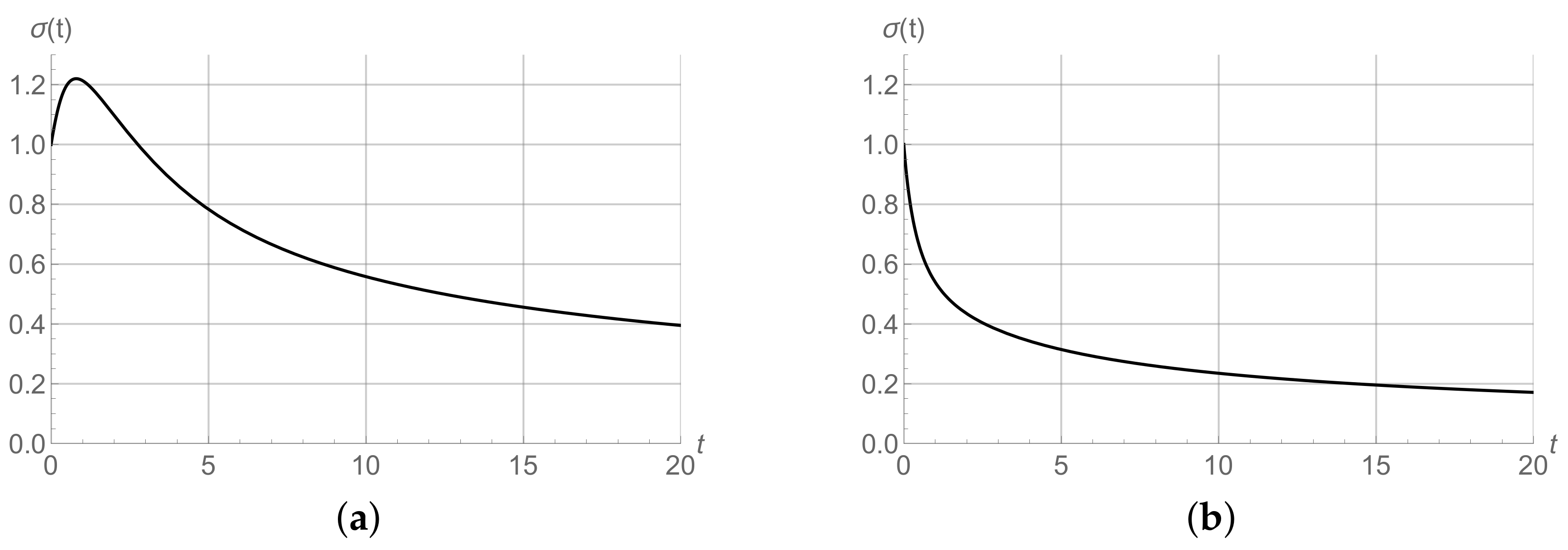
Since the function (58), (59) is given by the quite complex expression involving incomplete gamma functions, it has a number of behavior types depending on parameters. We will focus on ones satisfying (69). The solution $\sigma \left(t\right)$ (58), (59) can have two essentially different behavior types. If the remanent temperature of electrons is sufficient for the excess ionization, then $\sigma \left(t\right)$ is the function with a single maximum point and the asymptote $\sigma =0$. In Figure 1a, the plot of such the function is shown for $\varkappa =2$, $\varrho =0.5$, ${\tau }_a={\tau }_b={\tau }_d=1$, $A_1=1$, $d_1=2$, $B_2=0.4$, $B_1=0.2$, $D=0.01$, $D_{in}=0.01$, $\sigma \left(0\right)=1$. If the initial electron temperature is sufficiently small, then the function $\sigma \left(t\right)$ monotonically decrease tending to zero. This case is shown in Figure 1b for same parameters except for $A_1=0.3$, $B_2=2$, $B_1=1$.

The bifurcation of behavior types is determined by the sign of the number I given by

$${\displaystyle I=A_1-\varkappa {\sigma }^2\left(0\right)B_1\left[1-4\frac{D_{i}n}{{\varrho }^2}\right]=A_1-\varkappa {\sigma }^2\left(0\right)B_1+\mathrm{O}\left(D\right).}$$

(70)

Thus, the condition $I>0$ ensures the presence of the excess ionization.

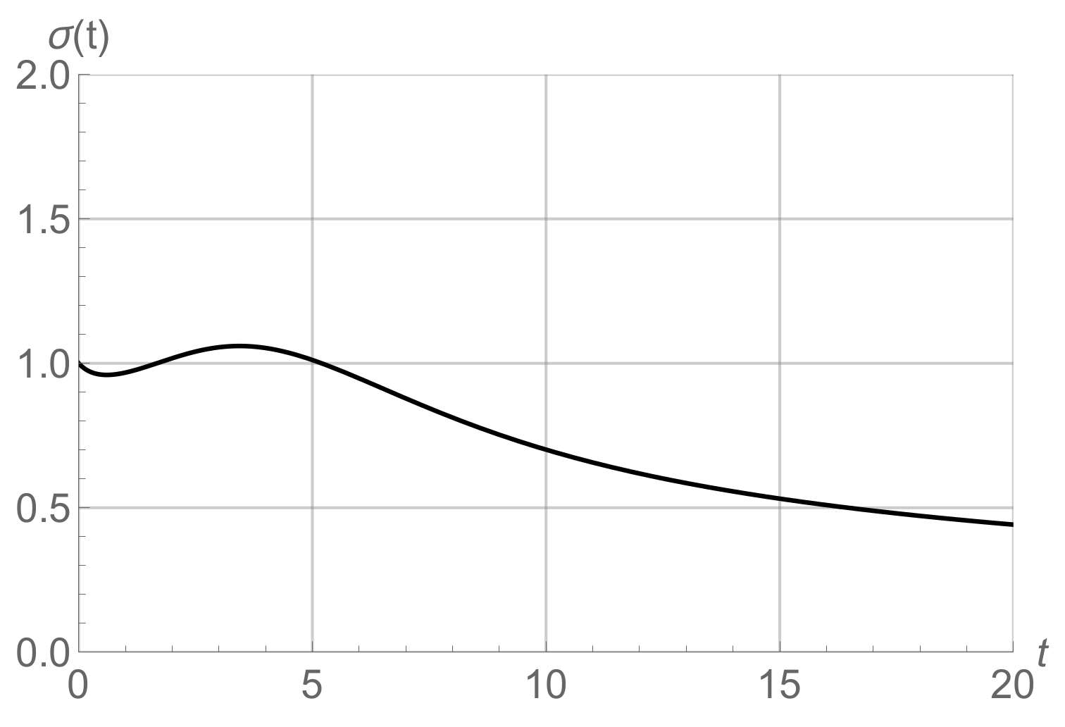
The Formulas (58) and (59) also admit one more kind of solution satisfying (69), which is shown in Figure 2 for the same parameters as in Figure 1b except for $A_1=1.5$, ${\tau }_a={\tau }_b=2$, ${\tau }_d=1$, $d_1=2.5$.

The solution in Figure 2 have two extreme points. The prerequisite for such the case is that the condition

$${\displaystyle \left\{\begin{array}{c}\dot{\sigma }\left(t\right)=0\hfill \\ \ddot{\sigma }\left(t\right)\ge 0\hfill \end{array}\right.⟹\frac{d}{dt}\frac{{\displaystyle \beta \left(t\right)\left[1-4\frac{D_{in}}{{\varrho }^2}-8\frac{D}{{\varrho }^2}\underset{0}{\overset{t}{\int }}{\tilde{D}}_a\left(\tau \right)d\tau \right]}}{\tilde{a}\left(t\right)}\le 0}$$

(71)

holds for some t. For $D\to 0$, the condition (71) yields

$${\displaystyle \frac{d}{dt}\frac{\beta \left(t\right)}{\tilde{a}\left(t\right)}\le 0,}$$

(72)

that contradicts assumptions for the functions $\tilde{a}\left(t\right)$, $\beta \left(t\right)$ leading to (57). Therefore, the case shown in Figure 2 is not of interest in the weak diffusion approximation and the sign of I unequivocally determines the choice between cases shown in Figure 1a,b.

6. Conclusions

We have developed an approximate analytical approach based on the WKB–Maslov theory [25,26,27] for studying kinetic phenomena in an active medium on metal vapors under the condition of quasi-neutrality in terms of the nonlocal kinetic Equation (5). The key point of the approach is the use of the class ${\mathcal{P}}_D^t$ of trajectory concentrated functions given by (8) in which the solution to the Cauchy problem of Equation (5) is sought. This allows us to reduce the Cauchy problem for the kinetic Equation (5) to the solution of the corresponding Cauchy problem for the associated linear Equation (40) or (42), using the general solution (32) of the EE system (26) of moments of the desired solution. As a result, we obtain the leading term of the asymptotic solution of the Cauchy problem for the kinetic Equation (5) accurate to $\mathrm{O}\left(D^{3/2}\right)$ in the weak diffusion approximation.

Since the numerous publications dedicated to the kinetic modeling of MVAM are mainly focused on numerical study, our approach can be used both for the approval of complex numerical models and as an independent method for calculation of the electron density in MVAM within given approximations.

The approach proposed here can be considered as an extension of the method of semiclassical asymptotics in the class of functions ${\mathcal{P}}_D^t$, which we previously used in [28,30] for the population nonlocal Fisher–Kolmogorov–Petrovskii–Piskunov (Fisher–KPP) equation and for the nonlocal Gross–Pitaevskii equation in [31,32].

The solutions of the Equation (7) obtained in this work have similarities with solutions of the Fisher–KPP equation constructed in [28,30] for the one-dimensional case since these equations have the same set of stationary points for the spatially uniform functions $u\ge 0$: one unstable stationary point $u=0$ and one stable stationary point $u>0$.

Nevertheless, the cubic nonlinearities leads to some distinctions. In particular, the zeroth-order moment $\sigma \left(t\right)$ in (58), (59) for solutions (67) cannot take on a negative value for the positive initial condition while it could be for the asymptotic solutions of the Fisher–KPP equation with the quadratic nonlinearity [30]. Since the zeroth-order moment corresponds to the population density in the Fisher–KPP model, it is not trivial how to interpret such the solutions from the physical point of view. The absence of this issue for the semiclassical approach to the model considered in this work means that this approach is more natural for the equation with the cubic nonlinearity. In this sense, the Equation (7) is similar to the Gross–Pitaevskii equation [31,32].

The plasma relaxation problem considered in Section 5 within the framework of the proposed method illustrates the construction of the leading term of the semiclassical asymptotics for the kinetic Equation (5) in explicit form using the incomplete gamma function. With the help of the solution constructed, the time dependence of the number of ions $\sigma \left(t\right)$, which is an important characteristic of plasma kinetics, was obtained explicitly and analyzed. It is shown that the solution can correspond to the relaxation process with or without the excess ionization depending on the problem setup.

It can be seen from the results obtained that the WKB–Maslov method of semiclassical asymptotics can be certainly applied to the nonlocal generalization of the FitzHugh–Nagumo model [36,37] in the similar way as it was used for the two-component Fisher–KPP equation in [38] and to the nonlocal generalization of the Zeldovich–Frank–Kamenetskii equation [39]. However, we expect the essentially different solution behavior for them since those equations have different set of stationary points.

References

- Kazaryan, M.A.; Lyabin, N.A.; Zharikov, V.M. Technological systems based on copper vapor laser designed for measurement and material processing. In Seventh International Symposium on Laser Metrology Applied to Science, Industry, and Everyday Life; Chugui, Y.V., Bagayev, S.N., Weckenmann, A., Osanna, P.H., Eds.; International Society for Optics and Photonics: Bellingham, WA, USA, 2002; Volume 4900, pp. 1094–1098. [Google Scholar]
- Asratyan, A.A.; Bulychev, N.A.; Feofanov, I.N.; Kazaryan, M.A.; Krasovskii, V.I.; Lyabin, N.A.; Pogosyan, L.A.; Sachkov, V.I.; Zakharyan, R.A. Laser processing with specially designed laser beam. Appl. Phys. A Mater. Sci. Process. 2016, 122, 434. [Google Scholar] [CrossRef]
- Klyuchareva, S.V.; Ponomarev, I.V.; Topchiy, S.B.; Pushkareva, A.E.; Andrusenko, Y.N. Treatment of basal cell cancer with a pulsed copper vapor laser: A case series. J. Lasers Med Sci. 2019, 10, 350–354. [Google Scholar] [CrossRef]
- Evtushenko, G.S.; Trigub, M.V.; Gubarev, F.A.; Evtushenko, T.G.; Torgaev, S.N.; Shiyanov, D.V. Laser monitor for non-destructive testing of materials and processes shielded by intensive background lighting. Rev. Sci. Instrum. 2014, 85, 033111. [Google Scholar] [CrossRef]
- Trigub, M.V.; Torgaev, S.N.; Evtushenko, G.S.; Troitskii, V.O.; Shiyanov, D.V. A bistatic laser monitor. Tech. Phys. Lett. 2016, 42, 632–634. [Google Scholar] [CrossRef]
- Evtushenko, G.S.; Torgaev, S.N.; Trigub, M.V.; Shiyanov, D.V.; Evtushenko, T.G.; Kulagin, A.E. High-speed CuBr brightness amplifier beam profile. Opt. Commun. 2017, 383, 148–152. [Google Scholar] [CrossRef]
- Gubarev, F.A.; Trigub, M.V.; Klenovskii, M.S.; Li, L.; Evtushenko, G.S. Radial distribution of radiation in a CuBr vapor brightness amplifier used in laser monitors. Appl. Phys. B Lasers Opt. 2016, 122, 2. [Google Scholar] [CrossRef]
- Mohammadpour Lima, S.; Behrouzinia, S.; Khorasani, K. Amplifying characteristics of small-bore copper bromide lasers. Appl. Phys. B Lasers Opt. 2019, 125, 1–5. [Google Scholar] [CrossRef]
- Boichenko, A.M.; Yakovlenko, S.I. Formation of high-quality radiation of a copper-vapor laser in a master oscillator-amplifier system. Laser Phys. 2005, 15, 1528–1535. [Google Scholar]
- Withford, M.J.; Brown, D.J.W.; Mildren, R.P.; Carman, R.J.; Marshall, G.D.; Piper, J.A. Advances in copper laser technology: Kinetic enhancement. Prog. Quantum Electron. 2004, 28, 165–196. [Google Scholar] [CrossRef]
- Kushner, M.J.; Warner, B.E. Large-bore copper-vapor lasers: Kinetics and scaling issues. J. Appl. Phys. 1983, 54, 2970–2982. [Google Scholar] [CrossRef]
- Newell, A.C.; Whitehead, J.A. Finite bandwidth, finite amplitude convection. J. Fluid Mech. 1969, 38, 279–303. [Google Scholar] [CrossRef] [Green Version]
- Vaneeva, O.; Boyko, V.; Zhalij, A.; Sophocleous, C. Classification of reduction operators and exact solutions of variable coefficient Newell–Whitehead–Segel equations. J. Math. Anal. Appl. 2019, 474, 264–275. [Google Scholar] [CrossRef] [Green Version]
- Freund, R.S.; Wetzel, R.C.; Shul, R.J.; Hayes, T.R. Cross-section measurements for electron-impact ionization of atoms. Phys. Rev. A 1990, 41, 3575–3595. [Google Scholar] [CrossRef] [PubMed]
- Gurevich, A.V.; Pitaevskii, L.P. Recombination coefficient in a dense low-temperature plasma. Sov. Phys. JETP 1964, 19. [Google Scholar]
- Carman, R.J.; Withford, M.J.; Brown, D.J.W.; Piper, J.A. Influence of the pre-pulse plasma electron density on the performance of elemental copper vapour lasers. Opt. Commun. 1998, 157, 99–104. [Google Scholar] [CrossRef]
- Boichenko, A.M.; Evtushenko, G.S.; Yakovlenko, S.I.; Zhdaniev, O.V. The influence of the initial density of metastable states and electron density on the pulse repetition rate in a copper-vapor laser. Laser Phys. 2001, 11, 580–588. [Google Scholar]
- Kyuregyan, A.S. Excitation of Copper Vapor Lasers by Storage Capacitor Direct Discharge via High-Speed Photothyristors. Opt. Spectrosc. 2019, 126, 388–393. [Google Scholar] [CrossRef]
- Borovich, B.L.; Yurchenko, N.I. Analysis of the excitation and relaxation kinetics in a copper vapor laser excited by a longitudinal discharge. Sov. J. Quantum Electron. 1984, 14, 1391–1400. [Google Scholar] [CrossRef]
- Carman, R.J.; Brown, D.J.W.; Piper, J.A. A Self Consistent Model for the Discharge Kinetics in a High-Repetition-Rate Copper-Vapor Laser. IEEE J. Quantum Electron. 1994, 30, 1876–1895. [Google Scholar] [CrossRef]
- Cheng, C.; Sun, W. Study on the kinetic mechanisms of copper vapor lasers with hydrogen-neon admixtures. Opt. Commun. 1997, 144, 109–117. [Google Scholar] [CrossRef]
- Kulagin, A.E.; Torgaev, S.N.; Evtushenko, G.S. Kinetic modeling of amplifying characteristics of copper vapor active media for a wide range of input radiation power. Opt. Commun. 2020, 460, 125136. [Google Scholar] [CrossRef]
- Torgaev, S.N.; Kulagin, A.E.; Evtushenko, T.G.; Evtushenko, G.S. Kinetic modeling of spatio-temporal evolution of the gain in copper vapor active media. Opt. Commun. 2019, 440, 146–149. [Google Scholar] [CrossRef]
- Kulagin, A.E.; Torgaev, S.N.; Evtushenko, G.S.; Trigub, M.V. Kinetics of the Active Medium of a Copper Vapor Brightness Amplifier. Russ. Phys. J. 2018, 60, 1987–1992. [Google Scholar] [CrossRef]
- Maslov, V. Operational Methods; Mir Publishers: Moscow, Russia, 1976. [Google Scholar]
- Maslov, V. The Complex WKB Method for Nonlinear Equations. I. Linear Theory; Birkhauser: Basel, Switzerland, 1994. [Google Scholar]
- Belov, V.V.; Dobrokhotov, S.Y. Semiclassical maslov asymptotics with complex phases. I. General approach. Theor. Math. Phys. 1992, 92, 843–868. [Google Scholar] [CrossRef]
- Trifonov, A.Y.; Shapovalov, A.V. The one-dimensional Fisher-Kolmogorov equation with a nonlocal nonlinearity in a semiclassical approximation. Russ. Phys. J. 2009, 52, 899–911. [Google Scholar] [CrossRef]
- Levchenko, E.A.; Shapovalov, A.V.; Trifonov, A.Y. Pattern formation in terms of semiclassically limited distribution on lower dimensional manifolds for the nonlocal Fisher-Kolmogorov-Petrovskii-Piskunov equation. J. Phys. A Math. Theor. 2014, 47, 025209. [Google Scholar] [CrossRef] [Green Version]
- Shapovalov, A.V.; Trifonov, A.Y. An application of the Maslov complex germ method to the one-dimensional nonlocal Fisher-KPP equation. Int. J. Geom. Methods Mod. Phys. 2018, 15, 1850102. [Google Scholar] [CrossRef]
- Belov, V.V.; Trifonov, A.Y.; Shapovalov, A.V. The trajectory-coherent approximation and the system of moments for the hartree type equation. Int. J. Math. Math. Sci. 2002, 32, 325–370. [Google Scholar] [CrossRef] [Green Version]
- Shapovalov, A.V.; Kulagin, A.E.; Trifonov, A.Y. The Gross–Pitaevskii equation with a nonlocal interaction in a semiclassical approximation on a curve. Symmetry 2020, 12, 201. [Google Scholar] [CrossRef] [Green Version]
- Kulagin, A.E.; Shapovalov, A.V.; Trifonov, A.Y. Semiclassical spectral series localized on a curve for the Gross–Pitaevskii equation with a nonlocal interaction. Symmetry 2021, 13, 1289. [Google Scholar] [CrossRef]
- Bagrov, V.G.; Belov, V.V.; Trifonov, A.Y. Semiclassical trajectory-coherent approximation in quantum mechanics I. High-order corrections to multidimensional time-dependent equations of Schrödinger type. Ann. Phys. 1996, 246, 231–290. [Google Scholar] [CrossRef]
- Levchenko, E.A.; Shapovalov, A.V.; Trifonov, A.Y. Asymptotics semiclassically concentrated on curves for the nonlocal Fisher-Kolmogorov-Petrovskii-Piskunov equation. J. Phys. A Math. Theor. 2016, 49, 305203. [Google Scholar] [CrossRef]
- FitzHugh, R. Impulses and Physiological States in Theoretical Models of Nerve Membrane. Biophys. J. 1961, 1, 445–466. [Google Scholar] [CrossRef] [Green Version]
- Nagumo, J.; Arimoto, S.; Yoshizawa, S. An Active Pulse Transmission Line Simulating Nerve Axon*. Proc. IRE 1962, 50, 2061–2070. [Google Scholar] [CrossRef]
- Shapovalov, A.V.; Trifonov, A.Y. Approximate solutions and symmetry of a two-component nonlocal reaction-diffusion population model of the Fisher-KPP type. Symmetry 2019, 11, 366. [Google Scholar] [CrossRef] [Green Version]
- Zeldovich, Y.B.; Barenblatt, G.I.; Librovich, V.B.; Makhviladze, G.M. The Mathematical Theory of Combustion and Explosions; Consultants Bureau: New York, NY, USA, 1985.
Figure 1.
The plot of the function for the high (a) and low (b) initial electron temperature.
Figure 2.
The plot of the function for the special case.
Publisher’s Note: MDPI stays neutral with regard to jurisdictional claims in published maps and institutional affiliations. |
© 2021 by the authors. Licensee MDPI, Basel, Switzerland. This article is an open access article distributed under the terms and conditions of the Creative Commons Attribution (CC BY) license (https://creativecommons.org/licenses/by/4.0/).
Share and Cite
MDPI and ACS Style
Shapovalov, A.V.; Kulagin, A.E. Semiclassical Approach to the Nonlocal Kinetic Model of Metal Vapor Active Media. Mathematics 2021, 9, 2995. https://0-doi-org.brum.beds.ac.uk/10.3390/math9232995
AMA Style
Shapovalov AV, Kulagin AE. Semiclassical Approach to the Nonlocal Kinetic Model of Metal Vapor Active Media. Mathematics. 2021; 9(23):2995. https://0-doi-org.brum.beds.ac.uk/10.3390/math9232995
Chicago/Turabian StyleShapovalov, Alexander V., and Anton E. Kulagin. 2021. "Semiclassical Approach to the Nonlocal Kinetic Model of Metal Vapor Active Media" Mathematics 9, no. 23: 2995. https://0-doi-org.brum.beds.ac.uk/10.3390/math9232995
Note that from the first issue of 2016, this journal uses article numbers instead of page numbers. See further details here.