The Meyers Estimates for Domains Perforated along the Boundary

Abstract

In this paper, we consider an elliptic problem in a domain perforated along the boundary. By setting a homogeneous Dirichlet condition on the boundary of the cavities and a homogeneous Neumann condition on the outer boundary of the domain, we prove higher integrability of the gradient of the solution to the problem.

1. Introduction

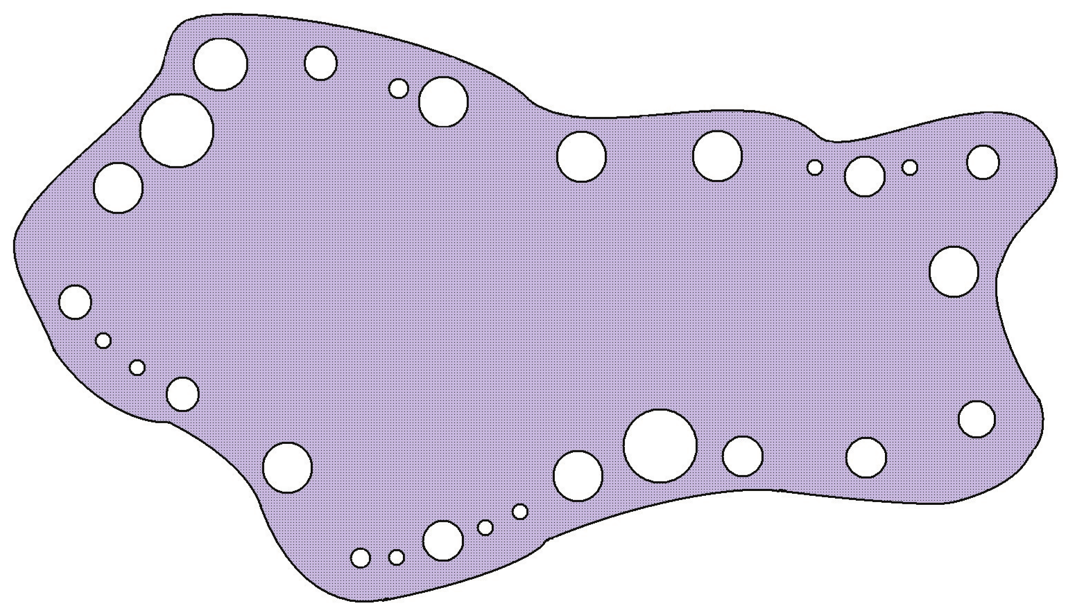
This paper confronts the estimates of solutions to an elliptic problem in domains perforated along the boundary (see Figure 1).

For the following homogeneous Dirichlet problem in a bounded domain:

$$\left\{\begin{array}{c}\mathcal{L}u:=\mathrm{div}\left(a\right(x)\nabla u)=\mathrm{div}f,x\in \mathsf{\Omega },\hfill \\ u=0,x\in \partial \mathsf{\Omega }\hfill \end{array}\right.$$

(1)

with uniformly elliptic measurable and symmetric matrix $a\left(x\right)$, that is, $a_{ij}=a_{ji}$, and the following:

$${\lambda }^{-1}{|\xi |}^2\le \sum _{i,j=1}^d{a}_{ij}\left(x\right){\xi }_i{\xi }_j\le \lambda {|\xi |}^2,\mathrm{for}\mathrm{almost}\mathrm{all}x\in \mathsf{\Omega },\mathrm{and}\mathrm{for}\mathrm{all}\xi \in {\mathbb{R}}^d,$$

(2)

and with the right hand side as $f\in L_p\left(\mathsf{\Omega }\right)$, where $p>2$, a higher integrability of the gradient of solutions (Meyers estimates) in a plane domain was proved in [1]. In other words, it was proved that the gradient of the solution is integrable at the power greater than two:

$$\underset{\mathsf{\Omega }}{\int }|\nabla u_{\epsilon }{|}^{2+\delta }dx\le C\underset{\mathsf{\Omega }}{\int }{|f|}^{2+\delta }dx.$$

(3)

In a multidimensional case, the same result for domains with sufficiently smooth boundary was proved in [2]. It should be noted that higher integrability of the gradient of solutions to the Dirichlet problem in a bounded domain with Lipschitz boundary for p-Laplacian with variable p was obtained in [3].

The Meyers estimate (higher integrability) of solutions to a Zaremba problem with rapidly changing type of boundary conditions in a plane domain for the Laplacian can be observed in [4]. The uniformly elliptic operators in the multidimensional case can be observed in [5].

Some other integral estimates of solutions can be found in [6,7,8,9]. In paper [10], one can find the integral estimates in domains perforated along the boundary.

It should be noted that similar mathematical models and problems appear in many applications, for instance, in mechanics of aircraft and space structures, theory of bridge constructions, hudrodynamics of bodies with complicated microstructure, etc. For more details, refer to [11].

This paper is devoted to obtaining the Meyers estimates for the gradient of the solution to an elliptic problem on a perforated slope along the boundary. Thus, by assuming a homogeneous Dirichlet condition at the cavity boundary and a Neumann homogeneous condition at the outer boundary of the domain, higher integrability of the gradient of the solution is proved.

2. Setting of the Problem and Formulation of the Main Result

Consider a domain $\mathsf{\Omega }\subset {\mathbb{R}}^d$, $d\ge 2$, with Lipschitz boundary (Lipschitz domain). Denote by ${\mathsf{\Gamma }}_{\epsilon }$ the hypersurface lying in $\mathsf{\Omega }$ on the distance $\epsilon$ from the boundary $\partial \mathsf{\Omega }$. Here, $\epsilon >0$ is a small parameter. Suppose that $H_j^{\epsilon }$ are balls centered on this hypersurface with radii ${\alpha }_j\epsilon$, $0<{\alpha }_j<\frac{1}{2}$. Denote $H_{\epsilon }=\bigcup _{j\in J}{H}_j^{\epsilon }$, $J:=\{1,2,\dots ,M_{\epsilon }\}$. Here, $M_{\epsilon }$ is an integer and tends to infinity as $\epsilon \to 0$.

The domain $\mathsf{\Omega }$ is called a Lipschitz domain, if for any point $x_0\in \partial \mathsf{\Omega }$ there exists an open cube Q centered in $x_0$, with edges of the length $2R_0$ parallel to the coordinate axes such that $Q\cap \partial \mathsf{\Omega }$ is a graph of the Lipschitz function $x_n=g(x_1,\dots ,x_{n-1})$ with Lipschitz constant L independent of $x_0$. Here, $x=(x_1,\dots ,x_n)$ are new coordinates with origin in $x_0$.

Consider in the domain ${\mathsf{\Omega }}_{\epsilon }:=\mathsf{\Omega }\backslash \overline{H_{\epsilon }}$, the following problem:

$$\left\{\begin{array}{c}\mathcal{L}{u}_{\epsilon }=\mathrm{div}f,\mathrm{in}{\mathsf{\Omega }}_{\epsilon },\hfill \\ u_{\epsilon }=0,\mathrm{on}\partial H_{\epsilon },\hfill \\ \frac{\partial u_{\epsilon }}{\partial n}=0,\mathrm{on}\partial \mathsf{\Omega },\hfill \end{array}\right.$$

(4)

where $\frac{\partial u_{\epsilon }}{\partial n}$ is an outward conormal derivative of the function $u_{\epsilon }$, and the components of the vector-function $f=(f_1,\dots ,f_d)$ are functions from $L_2\left(\mathsf{\Omega }\right)$. In order to define the solution to problem (4) denoted by $W_2^1({\mathsf{\Omega }}_{\epsilon },H_{\epsilon })$, the completion of the set of infinitely smooth functions in $\overline{\mathsf{\Omega }}$ is required, vanishing in the vicinity of $\partial H_{\epsilon }$, with respect to the following norm.

$${\Vert u\Vert }_{W_2^1({\mathsf{\Omega }}_{\epsilon },H_{\epsilon })}={\left(\underset{{\mathsf{\Omega }}_{\epsilon }}{\int }{u}^{2}dx+\underset{{\mathsf{\Omega }}_{\epsilon }}{\int }{|\nabla u|}^{2}dx\right)}^{1/2}.$$

The function $u_{\epsilon }\in W_2^1({\mathsf{\Omega }}_{\epsilon },H_{\epsilon })$ is called a solution to problem (4), if the following integral identity:

$$\underset{{\mathsf{\Omega }}_{\epsilon }}{\int }a\nabla u_{\epsilon }·\nabla \phi dx=\underset{{\mathsf{\Omega }}_{\epsilon }}{\int }f·\nabla \phi dx,$$

(5)

holds for any test–function $\phi \in W_2^1({\mathsf{\Omega }}_{\epsilon },H_{\epsilon })$ (see [12,13]).

We now study the question of higher integrability of the gradient of the solution to problem (4).

Let us describe the structure of the set $\partial H_{\epsilon }$. Consider a compact set $K\subset {\mathbb{R}}^d$. Define the capacity $C_p\left(K\right)$ for $1<p<d$ by the following formula.

$$C_p\left(K\right)=inf\left\{\underset{{\mathbb{R}}^d}{\int }{|\nabla \phi |}^{p}dx:\phi \in C_0^{\infty }\left({\mathbb{R}}^d\right),\phi \ge 1\mathrm{on}K\right\}.$$

(6)

Let $B_r^{x_0}$ be an open ball centered in $x_0$ with radius r, and let $me{s}_{d-1}\left(E\right)$ be $(d-1)$-dimensional measure of the set E (see for the definition, for instance [14]). Assume that the following is the case.

$$p=\frac{2d}{d+2},\mathrm{as}d>2,p=\frac{3}{2},\mathrm{as}d=2.$$

Denote by $F_s$ the boundary layer along the boundary $\partial \mathsf{\Omega }$ with a thickness that equals to $s\ge \frac{3}{2}\epsilon$, including all the cavities.

Suppose that for $x_0\in F_{\frac{3}{2}\epsilon }$ and $r\le r_0$, either we have the following inequality:

$$C_p(\partial H_{\epsilon }\cap {\overline{B}}_r^{x_0})\ge c_0{r}^{d-p},$$

(7)

or the the following inequality:

$$me{s}_{d-1}(\partial H_{\epsilon }\cap {\overline{B}}_r^{x_0})\ge c_0{r}^{d-1},$$

(8)

where the positive constant $c_0$ does not depend on $x_0$ and r.

Note that the condition (8) is stronger but is easier to test. In addition, one can observe that under any of these conditions for any $v\in W_2^1({\mathsf{\Omega }}_{\epsilon },H_{\epsilon })$, the Friedrichs inequality of the following:

$$\underset{{\mathsf{\Omega }}_{\epsilon }}{\int }{v}^{2}dx\le K\underset{{\mathsf{\Omega }}_{\epsilon }}{\int }{|\nabla v|}^{2}dx,$$

holds, which by means of the Lax–Milgram Lemma (see [15]) results in the existence of a unique solution to problem (4).

Theorem 1.

If $f\in L_{2+{\delta }_0}\left(\mathsf{\Omega }\right)$, where ${\delta }_0>0$, then there exist positive constants $\delta (d,{\delta }_0)<{\delta }_0$ and C in that the solution to problem (4) satisfies Lax-Milgra estimate:

$$\underset{{\mathsf{\Omega }}_{\epsilon }}{\int }|\nabla u_{\epsilon }{|}^{2+\delta }dx\le C\underset{{\mathsf{\Omega }}_{\epsilon }}{\int }{|f|}^{2+\delta }dx,$$

(9)

where C depends only on ${\delta }_0$, d and $c_0$ from (7) and (8), the constant λ and also on $r_0\le R_0$ and L.

3. Proof of the Main Result

Proof of Theorem 1.

First of all we estimate the gradient of a solution to problem (2) in the neighbourhood of the boundary of the domain. Let us locally transform the coordinates in the vicinity of the boundary and, more precisly, in the neighbourhood of an arbitrary point $x_0\in \partial \mathsf{\Omega }$. By denoting the following:

$$Q_{R_0}=\{x:|x_i|<R_0,i=1,\dots ,d\},$$

consider a local Cartesian coordinate system with its origin in $x_0$ and that $\partial \mathsf{\Omega }\cap Q_{R_0}$ is given in this coordinate system by the following equation:

$$x_d=g\left(x^{\prime }\right),x^{\prime }=(x_1,\dots ,x_{d-1}),$$

where g is a Lipschitz function with the Lipschitz constant L. We assume that the following:

$${\mathsf{\Omega }}_{\epsilon ,R_0}=Q_{R_0}\cap \mathsf{\Omega }\epsilon ,$$

satisfies $x_d>g\left(x^{\prime }\right)$. By changing the following variables:

$$y^{\prime }=x^{\prime },y_d=x_d-g\left(x^{\prime }\right),$$

(10)

we have the following:

$$P_{R_0}=\{y:|y_i|<R_0,i=1,\dots ,d-1,y_d=0\},$$

for $Q_{R_0}\cap \partial \mathsf{\Omega }$. Denote by ${\tilde{Q}}_{R_0}$ the domain $Q_{R_0}$ after the transformation of the coordinates $x\mapsto y$ (see Figure 2). □

Lemma 1.

The domain ${\tilde{Q}}_{R_0}$ contains the following cube.

$$K_{R_0}=\{y:|y_i|<{(1+\sqrt{d-1}L)}^{-1}{R}_0,i=1,\dots ,d\}.$$

(11)

Proof. 

Suppose that $y\in {\tilde{Q}}_{R_0}$ and $|y_i|<\vartheta R_0$ for some $\vartheta \in (0,1)$ and $i=1,\dots ,d-1$. It is easy to observe that the following is the case:

$$y_d\in (-R_0-g\left(y^{\prime }\right),R_0-g\left(y^{\prime }\right)).$$

due to the fact that function g is Lipschitz and $g\left(0\right)=0$; thus, we have the following.

$$|g\left(y^{\prime }\right)|\le L|y^{\prime }|<\sqrt{n-1}L\vartheta R_0.$$

Consequently, the following is the case.

$$(-R_0(1-\sqrt{n-1}L\delta ),R_0(1-\sqrt{n-1}L\delta ))\subset (-R_0-g\left(y^{\prime }\right),R_0-g\left(y^{\prime }\right)).$$

Moreover, by taking the following:

$$\vartheta =\frac{1}{1+L\sqrt{d-1}},$$

we complete the proof. □

Now problem (2) in perforated semicube $K_{R_0,\mathrm{perf}}^{+}=K_{R_0}\cap {\tilde{\mathsf{\Omega }}}_{\epsilon }$ has the following form.

$$\left\{\begin{array}{c}\tilde{\mathcal{L}}{v}_{\epsilon }=\mathrm{div}\tilde{f},\mathrm{in}{K}_{R_0,\mathrm{perf}}^{+},\hfill \\ v_{\epsilon }=0,\mathrm{on}\partial {\tilde{H}}_{\epsilon }\cap K_{R_0},\hfill \\ \frac{\partial v_{\epsilon }}{\partial \tilde{n}}=0,\mathrm{on}\partial \tilde{\mathsf{\Omega }}\cap K_{R_0}.\hfill \end{array}\right.$$

(12)

Here, $\tilde{\mathsf{\Omega }}$, ${\tilde{\mathsf{\Omega }}}_{\epsilon }$ and ${\tilde{H}}_{\epsilon }$ are the images under transformation (10) of the domains $\mathsf{\Omega }$, ${\mathsf{\Omega }}_{\epsilon }$ and $H_{\epsilon }$, respectively, and the following:

$$\tilde{\mathcal{L}}v:=\mathrm{div}(b\left(y\right)\nabla v),$$

(13)

satisfies $b_{ij}=b_{ji}$ and

$${\mu }^{-1}{|\xi |}^2\le \sum _{i,j=1}^d{b}_{ij}\left(y\right){\xi }_i{\xi }_j\le \mu {|\xi |}^2,\mathrm{for} \mathrm{almost} \mathrm{all}y\in K_{R_0}^{+},\mathrm{and} \mathrm{for} \mathrm{all}\xi \in {\mathbb{R}}^d,$$

(14)

where $\mu$ depends on $\lambda$ from (1) and the constant L of the function g. Note that the following is the case:

$$\begin{array}{c}\hfill {\displaystyle \tilde{f}\left(y\right)=({\tilde{f}}_1\left(y\right),\dots ,{\tilde{f}}_d\left(y\right)),\mathrm{where}{\tilde{f}}_i\left(y\right)=f_i(y^{\prime },y_d+g\left(y^{\prime }\right)),\mathrm{as}i=1,\dots ,d-1},\\ \hfill {\displaystyle {\tilde{f}}_d\left(y\right)=\sum _{i=1}^{d-1}\frac{\partial g\left(y^{\prime }\right)}{\partial y_i}{f}_i(y^{\prime },y_d+g\left(y^{\prime }\right))+f_d(y^{\prime },y_d+g\left(y^{\prime }\right))},\end{array}$$

(15)

and $\frac{\partial v_{\epsilon }}{\partial \tilde{n}}$ is the respective conormal derivative.

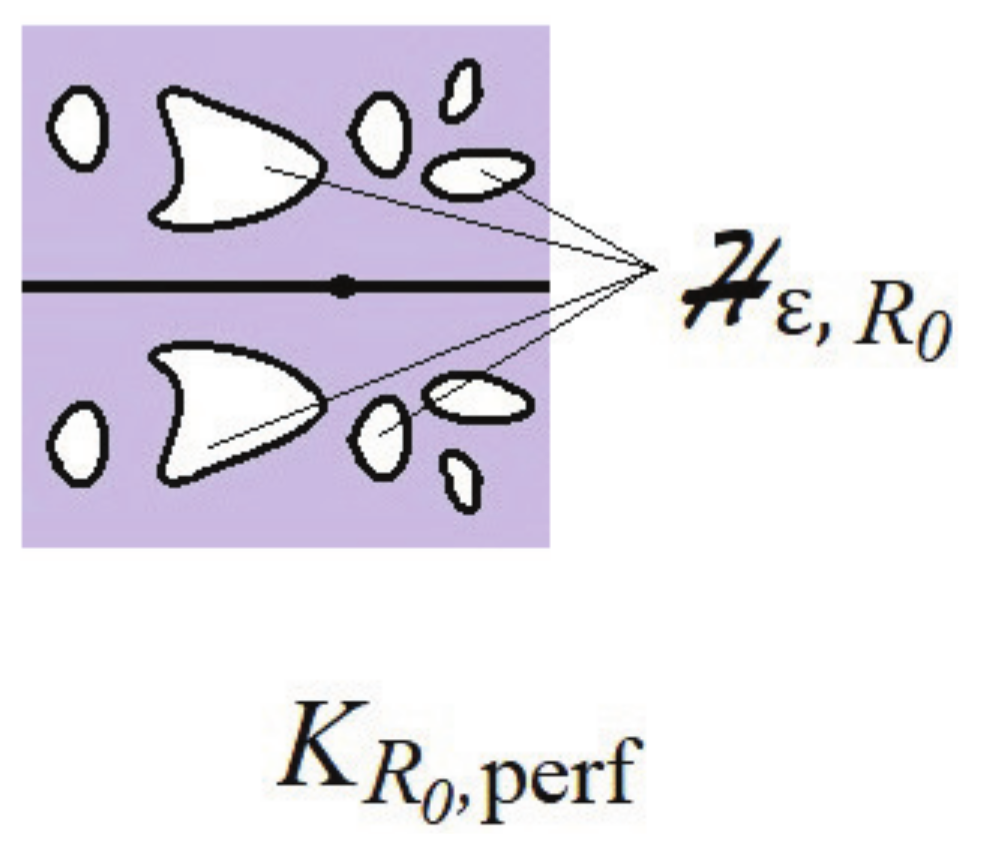
Denote by $K_{R_0,\mathrm{perf}}^{-}$ the domain $\{y:(y_1,\dots ,y_{d-1},-y_d)\in K_{R_0,\mathrm{perf}}^{+}\}$, and let $K_{R_0,\mathrm{perf}}$ be the union $K_{R_0,\mathrm{perf}}^{-}\cup K_{R_0,\mathrm{perf}}^{+}$. Denote also by ${\mathcal{H}}_{\epsilon ,R_0}$ the cavities (pores) in $K_{R_0,\mathrm{perf}}$ (see Figure 3).

Let us extend the solution $v_{\epsilon }$ to problem (12) by zero inside the pores and then extend it with respect to the hyperplane $\{y:y_d=0\}$. We retain the same notation for the extended function. The extended function $v_{\epsilon }$ satisfies the following problem.

$$\left\{\begin{array}{c}{\tilde{\mathcal{L}}}_1{v}_{\epsilon }=\mathrm{div}h,\mathrm{in}{K}_{R_0,\mathrm{perf}},\hfill \\ v_{\epsilon }=0,\mathrm{on}\partial {\mathcal{H}}_{\epsilon ,R_0}.\hfill \end{array}\right.$$

(16)

Here, we have the following:

$${\tilde{\mathcal{L}}}_{1}v:=\mathrm{div}(c\left(y\right)\nabla v),$$

with a positive definite matrix $c=\left\{c_{ij}\left(y\right)\right\}$ satisfying $c_{jd}\left(y\right)=c_{dj}\left(y\right)$, as $j\ne d$. Moreover, $c_{jd}$ are odd extensions of the functions $b_{jd}\left(y\right)$ from (13), and $c_{ij}\left(y\right)$ are even extensions of $b_{ij}\left(y\right)$, $j\ne d$. The vector function $h=(h_1,\dots ,h_d)$ in (16) is defined by the following relations: $h_i\left(y\right)$ as $i=1,\dots ,d-1$, are the even extension of the components ${\tilde{f}}_i\left(y\right)$ from (12), and $h_d\left(y\right)$ is the odd extension of ${\tilde{f}}_d\left(y\right)$.

Clearly the solution to problem (16) is the function $v_{\epsilon }\in W_2^1(K_{R_0,\mathrm{perf}},{\mathcal{H}}_{\epsilon ,R_0})$, which satisfies the integral identity (see (5)):

$$\underset{K_{R_0,\mathrm{perf}}}{\int }c\left(y\right)\nabla v_{\epsilon }·\nabla \phi dy=\underset{K_{R_0,\mathrm{perf}}}{\int }h·\nabla \phi dy,$$

(17)

for any $\phi \in W_2^1(K_{R_0,\mathrm{perf}},{\mathcal{H}}_{\epsilon ,R_0})$. Here, $W_2^1(K_{R_0,\mathrm{perf}},{\mathcal{H}}_{\epsilon ,R_0})$ is the closure of the set of infinitely smooth functions in $K_{R_0,\mathrm{perf}}$, vanishing in a vicinity of $\partial K_{R_0}$ and $\partial {\mathcal{H}}_{\epsilon ,R_0}$ by the following norm.

$${\Vert u\Vert }_{W_2^1(K_{R_0,\mathrm{perf}},{\mathcal{H}}_{\epsilon ,R_0})}={\left(\underset{K_{R_0,\mathrm{perf}}}{\int }{u}^{2}dx+\underset{K_{R_0,\mathrm{perf}}}{\int }{|\nabla u|}^{2}dx\right)}^{1/2}.$$

We denote by $Q_R^{y_0}$ the open cube centered in $y_0$ with edges of the length $2R$ parallel to the coordinate axes. Moreover, we assume that the following is the case.

$$y_0\in K_{\frac{R_0}{2}}\backslash \partial K_{\frac{R_0}{2}},\mathrm{where}R\le \frac{1}{2}dist(y_0,\partial K_{\frac{R_0}{2}}).$$

Denote the following:

$$\underset{Q_R^{y_0}}{\sout{\int }}wdx=\frac{1}{|Q_R^{y_0}|}\underset{Q_R^{y_0}}{\int }wdx,$$

where $|Q_R^{y_0}|$ is the d-dimensional measure of the cube $Q_R^{y_0}$.

• Consider the case $Q_{\frac{3R}{2}}^{y_0}\subset K_{R_0,\mathrm{perf}}$ and take in (17) the test-function $\phi =(v_{\epsilon }-\varpi ){\eta }^2$, where the following is the case.

  $$\varpi =\underset{Q_{\frac{3R}{2}}^{y_0}}{\sout{\int }}{v}_{\epsilon },dy.$$

  (18)

  Here, the cutoff function $\eta \in C_0^{\infty }\left(Q_{\frac{3R}{2}}^{y_0}\right)$ satisfies the following.

  $$0<\eta \le 1,\eta =1,\mathrm{in}{Q}_R^{y_0},\mathrm{and}|\nabla \eta |\le \frac{C}{R}.$$

  (19)

  Next, the lemma is devoted to the Caccioppoli inequality.

  Lemma 2.

  For the solution $v_{\epsilon }$ to problem (16), the following Caccioppoli inequality:

  $$\underset{Q_R^{y_0}}{\int }{|\nabla v_{\epsilon }|}^{2}dy\le C(d,\lambda ,L)\left(\frac{1}{R^2}\underset{Q_{\frac{3R}{2}}^{y_0}}{\int }{(v_{\epsilon }-\varpi )}^{2}dy+\underset{Q_{\frac{3R}{2}}^{y_0}}{\int }{|h|}^{2}dy\right),$$

  (20)

  holds true with φ defined in (18).

  Proof 

  By taking $\eta$ defined in (19) and substituting the test function $\phi =(v_{\epsilon }-\varpi ){\eta }^2$ in the integral identity (17), we have the following.

  $$\begin{array}{cc}\hfill \underset{Q_{\frac{3R}{2}}^{y_0}}{\int }c\left(y\right){|\nabla v_{\epsilon }|}^2{\eta }^{2}dy=& -2\underset{Q_{\frac{3R}{2}}^{y_0}}{\int }c\left(y\right)\eta (v_{\epsilon }-\varpi )\nabla v_{\epsilon }·\nabla \eta dy+\underset{Q_{\frac{3R}{2}}^{y_0}}{\int }{\eta }^{2}h·\nabla v_{\epsilon }dy+\hfill \\ \hfill & +2\underset{Q_{\frac{3R}{2}}^{y_0}}{\int }\eta (v_{\epsilon }-\varpi )h·\nabla \eta dy.\hfill \end{array}$$

  (21)

  Since $0\le \eta \le 1$, then by inequality $a^2+b^2\ge 2ab$, we derive the following.

  $$\begin{array}{cc}\hfill |\eta (v_{\epsilon }-\varpi )\nabla v_{\epsilon }·\nabla \eta |& \le \frac{1}{16}|\nabla v_{\epsilon }{|}^2{\eta }^2+4{(v_{\epsilon }-\varpi )}^2{|\nabla \eta |}^2,\hfill \\ \hfill |{\eta }^{2}h·\nabla v_{\epsilon }|& \le \frac{1}{16}|\nabla v_{\epsilon }{|}^2{\eta }^2+4{|h|}^2,\hfill \\ \hfill |\eta (v_{\epsilon }-\varpi )h·\nabla \eta |& \le \frac{1}{16}{|h|}^2+4{(v_{\epsilon }-\varpi )}^2{|\nabla \eta |}^2.\hfill \end{array}$$

  (22)

  Using the inequalities (21) and (22) and the ellipticity of problem (16), we obtain the following.

  $$\underset{Q_{\frac{3R}{2}}^{y_0}}{\int }{|\nabla v_{\epsilon }|}^2{\eta }^{2}dx\le C\left(\underset{Q_{\frac{3R}{2}}^{y_0}}{\int }{(v_{\epsilon }-\varpi )}^2{|\nabla \eta |}^{2}dx+\underset{Q_{\frac{3R}{2}}^{y_0}}{\int }{|h|}^{2}dx\right).$$

  (23)

  Finally, bearing in mind that $\eta =1$ in $Q_R^{y_0}$ and $|\nabla \eta |\le \frac{C}{R}$, we obtain inequality (20). The lemma is proved. □

  Then, by using the Poincaré–Sobolev inequality:

  $${\left(\underset{Q_{\frac{3R}{2}}^{y_0}}{\sout{\int }}{(v_{\epsilon }-\varpi )}^{2}dx\right)}^{1/2}\le C(d,p)R{\left(\underset{Q_{\frac{3R}{2}}^{y_0}}{\sout{\int }}{|\nabla v_{\epsilon }|}^{p}dx\right)}^{1/p},$$

  with $p\ge \frac{2d}{d+2}$, we deduce from (23) the following.

  $${\left(\underset{Q_R^{y_0}}{\sout{\int }}{|\nabla v_{\epsilon }|}^{2}dy\right)}^{1/2}\le C(d,\lambda ,L,p)\left({\left(\underset{Q_{2R}^{y_0}}{\sout{\int }}{|\nabla v_{\epsilon }|}^{p}dy\right)}^{1/p}+{\left(\underset{Q_{2R}^{y_0}}{\sout{\int }}{|h|}^{2}dy\right)}^{1/2}\right).$$

  (24)
• Consider the case $Q_{\frac{3R}{2}}^{y_0}\cap {\mathcal{H}}_{\epsilon ,R_0}\ne \varnothing$. Taking in (17) the test-function $\phi =v_{\epsilon }{\eta }^2$ with $\eta$ defined in (19), we come to (20) with $\varpi =0$; hence, we have the following.

  $$\underset{Q_R^{y_0}}{\int }{|\nabla v_{\epsilon }|}^{2}dy\le C(d,\lambda ,L,p)\left(\frac{1}{R^2}\underset{Q_{2R}^{y_0}}{\int }{v}_{\epsilon }^{2}dy+\underset{Q_{2R}^{y_0}}{\int }{|h|}^{2}dy\right).$$

  (25)

  Now, we estimate the first term in the right hand side of (25). If $Q_{\frac{3R}{2}}^{y_0}\cap {\mathcal{H}}_{\epsilon ,R_0}\ne \varnothing$, then there exists $z_0\in Q_{\frac{3R}{2}}^{y_0}\cap \partial {\mathcal{H}}_{\epsilon ,R_0}$ such that ${\overline{Q}}_{\frac{R}{2}}^{z_0}\subset {\overline{Q}}_{2R}^{y_0}$. Denote by z the pre-image (the inverse image) of point $z_0$ with respect to transformation (10). Note that the pre-image of the cube ${\overline{Q}}_{\frac{R}{2}}^{z_0}$ contains the ball ${\overline{B}}_{cR}^z$, with a positive constant c dependent on L and d. Due to (7), we have the following.

  $$C_p(\partial {\mathcal{H}}_{\epsilon ,R_0}\cap {\overline{B}}_{cR}^z)\ge C(L,d,c_0)R^{d-p}.$$

  Hence, by using the definition (6), we obtain $C_p(\partial {\mathcal{H}}_{\epsilon ,R_0}\cap {\overline{Q}}_{2R})\ge C(L,d,c_0)R^{d-p}$. Keeping in mind the imbedding theorem (see [1] (§14.1.2)), we estimate the following.

  $${\left(\underset{Q_{2R}^{y_0}}{\sout{\int }}{v}_{\epsilon }^{2}dy\right)}^{1/2}\le C(d,p,L,c_0)R(\underset{Q_{2R}^{y_0}}{\sout{\int }}{|\nabla v_{\epsilon }|}^{p}dy{)}^{1/p}.$$

  (26)

  If we use condition (8), then, bearing in mind the estimate from Proposition 4 from [1] (§13.1.1), we also obtain (26). Thus, estimate (25) results in inequality (24). Next, estimate (24) for any cubes $Q_R^{y_0}$ and the Gehring Lemma (see [16,17] and also [18] (Ch. VII)) produces the following inequality:

  $$\underset{K_{\frac{R_0}{4}}}{\int }|\nabla v_{\epsilon }{|}^{2+\delta }dy\le C(d,\lambda ,{\delta }_0,c_0,L,R_0)\underset{K_{\frac{R_0}{2}}}{\int }{|h|}^{2+\delta }dy,$$

  (27)

  if $h\in L_{2+{\delta }_0}\left(K_{R_0}\right)$, ${\delta }_0>0$, with positive constant $\delta =\delta (d,{\delta }_0)\le {\delta }_0$. Rewriting (27) and keeping in mind the properties of the extended functions, we have the following.

  $$\underset{K_{\frac{R_0}{4}}^{+}}{\int }|\nabla v_{\epsilon }{|}^{2+\delta }dy\le C(d,\lambda ,{\delta }_0,c_0,L,R_0)\underset{K_{\frac{R_0}{2}}^{+}}{\int }{|\tilde{f}|}^{2+\delta }dy.$$

  (28)

  Considering the inverse to (10) transformation, we conclude that the pre-image of $K_{\frac{R_0}{2}}$ is contained in ${\mathsf{\Omega }}_{\epsilon ,R_0}$, and the pre-image of cube $K_{\frac{R_0}{4}}^{+}$ contains the domain ${\mathsf{\Omega }}_{\epsilon ,\mu R_0}$, where $\mu =\mu (d,L)>0$. By means of (15) and (28), we obtain the following:

  $$\underset{{\mathsf{\Omega }}_{\epsilon ,\mu R_0}}{\int }|\nabla u_{\epsilon }{|}^{2+\delta }dx\le C(d,\lambda ,{\delta }_0,c_0,L,R_0)\underset{{\mathsf{\Omega }}_{\epsilon ,R_0}}{\int }{|f|}^{2+\delta }dx,$$

  or the following.

  $$\underset{{\mathsf{\Omega }}_{\epsilon }\cap Q_{\mu R_0}^{x_0}}{\int }|\nabla u_{\epsilon }{|}^{2+\delta }dx\le C(d,\lambda ,{\delta }_0,c_0,L,R_0)\underset{{\mathsf{\Omega }}_{\epsilon }\cap Q_{R_0}^{x_0}}{\int }{|f|}^{2+\delta }dx.$$

  Due to the arbitrariness of point $x_0\in \partial \mathsf{\Omega }$ and the compactness of boundary $\partial \mathsf{\Omega }$, one can find such finite cover of $\partial \mathsf{\Omega }$ such that the closed set:

  $${\mathsf{\Omega }}_{\epsilon ,{\mu }_1{R}_0}=\{x\in \mathsf{\Omega }:dist(x,\partial \mathsf{\Omega })\le {\mu }_1{R}_0\},{\mu }_1={\mu }_1(d,L)>0,$$

  is contained in the union of the sets ${\mathsf{\Omega }}_{\epsilon }\cap Q_{\mu R_0}^{x_i}$, where $x_i\in \partial \mathsf{\Omega }$. By summarizing the following inequalities:

  $$\underset{{\mathsf{\Omega }}_{\epsilon }\cap Q_{\mu R_0}^{x_i}}{\int }|\nabla u_{\epsilon }{|}^{2+\delta }dx\le C(d,\lambda ,{\delta }_0,c_0,L,R_0)\underset{{\mathsf{\Omega }}_{\epsilon }\cap Q_{R_0}^{x_i}}{\int }{|f|}^{2+\delta }dx,$$

  we derive the following.

  $$\underset{F_{{\mu }_1{R}_0}}{\int }|\nabla u_{\epsilon }{|}^{2+\delta }dx\le C(d,\lambda ,{\delta }_0,c_0,L,R_0)\underset{{\mathsf{\Omega }}_{\epsilon }}{\int }{|f|}^{2+\delta }dx.$$

  The internal estimate of the following:

  $$\underset{{\mathsf{\Omega }}_{\epsilon }\backslash F_{{\mu }_1{R}_0}}{\int }|\nabla u_{\epsilon }{|}^{2+\delta }dx\le C(d,\lambda ,{\delta }_0,R_0)\underset{{\mathsf{\Omega }}_{\epsilon }}{\int }{|f|}^{2+\delta }dx.$$

  follows from [2]. Finally, we have (9).

  Remark 1.

  Note that in the case $Q_{\frac{3R}{2}}^{y_0}\cap {\mathcal{H}}_{\epsilon ,R_0}\ne \varnothing$, when conditions (7) and (8) are not valid, we can modify the proof to obtain the same estimate (9). In this case, we also use Lemma 2, but instead of the Friedrichs–Sobolev inequality (26), we use the Poincaré–Sobolev inequality:

  $${\left(\underset{Q_{\frac{3R}{2}}^{y_0}}{\sout{\int }}{(v_{\epsilon }-\varpi )}^{2}dx\right)}^{1/2}\le C(d,p)R{\left(\underset{Q_{\frac{3R}{2}}^{y_0}}{\sout{\int }}{|\nabla v_{\epsilon }|}^{p}dx\right)}^{1/p},p\ge \frac{2d}{d+2},$$

  with an appropriate cutoff function.

4. One Application

Let us consider the following problem:

$$\left\{\begin{array}{c}\mathcal{L}{u}_{\epsilon }=\mathrm{div}f,\mathrm{in}{\mathsf{\Omega }}_{\epsilon },\hfill \\ u_{\epsilon }=0,\mathrm{on}\partial H_{\epsilon },\hfill \\ \frac{\partial u_{\epsilon }}{\partial n}+\varkappa u_{\epsilon }=0,\mathrm{on}\partial \mathsf{\Omega },\hfill \end{array}\right.$$

(29)

where $\varkappa$ is a constant in two-dimensional domain perforated along the boundary with the limit Robin (Fourier) problem of the following form.

$$\left\{\begin{array}{c}\mathcal{L}{u}_0=\mathrm{div}f,\mathrm{in}\mathsf{\Omega },\hfill \\ \frac{\partial u_0}{\partial n}+\varkappa u_0=0,\mathrm{on}\partial \mathsf{\Omega }.\hfill \end{array}\right.$$

(30)

Note that sequence $\left\{u_{\epsilon }\right\}$ is uniformly bounded in the Sobolev space $W_2^1$; hence, the existence of the limit function $u_0$ is obvious. We study the rate of convergence of the solution $u_{\epsilon }$ to solution $u_0$ in the Sobolev space $W_2^1$.

Assume that $(r_k,\theta )$ is the polar system of coordinates centered in $p_k^{\epsilon }$ (the center of the circle $H_k^{\epsilon }$). Consider the following cut-off function.

$${\psi }_{\epsilon }=\prod _k{\psi }_{\epsilon }^k,{\psi }_{\epsilon }^k=\psi \left(\frac{|ln\epsilon |}{|ln{r}_k|}\right),\psi \left(s\right)=\left\{\begin{array}{c}0,s\le 1,\hfill \\ 1,s\ge 1+\sigma .\hfill \end{array}\right.$$

Then, substitute the test-function ${\phi }_{\epsilon }={\psi }_{\epsilon }\phi$, $\phi \in W_2^1\left(\mathsf{\Omega }\right)$ in the integral identity of problem (29).

$$\underset{{\mathsf{\Omega }}_{\epsilon }}{\int }a\nabla u_{\epsilon }·\nabla {\phi }_{\epsilon }dx+\underset{\partial \mathsf{\Omega }}{\int }\varkappa u_{\epsilon }{\phi }_{\epsilon }ds=\underset{{\mathsf{\Omega }}_{\epsilon }}{\int }f·\nabla {\phi }_{\epsilon }dx,$$

(31)

In order to estimate the rate of convergence depending on $\epsilon \to 0$, we subtract the following integral identity:

$$\underset{\mathsf{\Omega }}{\int }a\nabla u_{\epsilon }·\nabla \phi dx+\underset{\partial \mathsf{\Omega }}{\int }\varkappa u_{\epsilon }\phi ds=\underset{\mathsf{\Omega }}{\int }f·\nabla \phi dx,\phi \in W_2^1\left(\mathsf{\Omega }\right),$$

(32)

of the limit problem (30) from integral identity (31). We obtain the following.

$$\begin{array}{c}\hfill \underset{\mathsf{\Omega }}{\int }a({\psi }_{\epsilon }\nabla u_{\epsilon }-\nabla u_0)·\nabla \phi dx+\underset{\partial \mathsf{\Omega }}{\int }\varkappa (u_{\epsilon }-u_0)\phi ds\\ \hfill =\underset{\mathsf{\Omega }}{\int }f·\nabla \phi ({\psi }_{\epsilon }-1)dx+\underset{\mathsf{\Omega }}{\int }a\nabla u_{\epsilon }·\nabla {\psi }_{\epsilon }\phi dx+\underset{\mathsf{\Omega }}{\int }f·\nabla {\psi }_{\epsilon }\phi dx.\end{array}$$

(33)

Rewriting (33) and keeping in mind the ellipticity of the operator $\mathcal{L}$ by means of the Cauchy inequality and the equivalence of the norms in the Sobolev space, we derive the following.

$$\begin{array}{c}\hfill \parallel u_{\epsilon }-u_0{\parallel }_{W_2^1\left(\mathsf{\Omega }\right)}^2\le C\left(\underset{\mathsf{\Omega }}{\int }f·\nabla \phi ({\psi }_{\epsilon }-1)dx+\underset{\mathsf{\Omega }}{\int }\nabla u_{\epsilon }·\nabla {\psi }_{\epsilon }dx\right).\end{array}$$

(34)

The first term in the right hand side of inequality (34) is easy to estimate (due to the Cauchy inequality) by the following.

$$K{M}_{\epsilon }^{\frac{1}{2}}{\epsilon }^{\frac{1}{1+\sigma }}.$$

Here, $M_{\epsilon }$ is the number of circles, and ${\epsilon }^{\frac{1}{1+\sigma }}$ is the diameter of the circle, where the integral is nontrivial, since ${\psi }_{\epsilon }-1\ne 0$.

Next, we estimate the second term at the right hand side of (34) and show the difference between inequalities with and without the Meyers estimate.

• Without Meyers
  We have the following.

  $$\begin{array}{c}\hfill {\displaystyle \underset{\mathsf{\Omega }}{\int }\nabla u_{\epsilon }·\nabla {\psi }_{\epsilon }dx\le {\left(\underset{\mathsf{\Omega }}{\int }{|\nabla u_{\epsilon }|}^{2}dx\right)}^{\frac{1}{2}}{\left(\underset{\mathsf{\Omega }}{\int }{|\nabla {\psi }_{\epsilon }|}^{2}dx\right)}^{\frac{1}{2}}}\\ \hfill \le K_1{M}_{\epsilon }^{\frac{1}{2}}|ln\epsilon |{\left(\underset{\epsilon }{\overset{{\epsilon }^{\frac{1}{1+\sigma }}}{\int }}{|lnr|}^{-4}dlnr\right)}^{\frac{1}{2}}\le K_2{M}_{\epsilon }^{\frac{1}{2}}{|ln\epsilon |}^{-\frac{1}{2}}.\end{array}$$
  The number of circles can be the following:

  $$M_{\epsilon }={|ln\epsilon |}^{1-\chi },$$

  where constant $\chi$ satisfies $0<\chi <1$. In this case, we have the final estimate.

  $$\begin{array}{c}\hfill \parallel u_{\epsilon }-u_0{\parallel }_{W_2^1\left(\mathsf{\Omega }\right)}^2\le C{|ln\epsilon |}^{-\frac{\chi }{2}}.\end{array}$$

  (35)
• With Meyers
  Suppose that the following is the case.

  $$p_1=2+\delta >2,p_2=\frac{2+\delta }{1+\delta }<2.$$

We obtain the following.

$$\begin{array}{c}\hfill {\displaystyle \underset{\mathsf{\Omega }}{\int }\nabla u_{\epsilon }·\nabla {\psi }_{\epsilon }dx\le {\left(\underset{\mathsf{\Omega }}{\int }{|\nabla u_{\epsilon }|}^{p_1}dx\right)}^{\frac{1}{p_1}}{\left(\underset{\mathsf{\Omega }}{\int }{|\nabla {\psi }_{\epsilon }|}^{p_2}dx\right)}^{\frac{1}{p_2}}}\\ \hfill \le K_1{M}_{\epsilon }^{\frac{1}{p_2}}{\epsilon }^{\frac{2-p_2}{p_2(1+\sigma )}}|ln\epsilon |{\left(\underset{\epsilon }{\overset{{\epsilon }^{\frac{1}{1+\sigma }}}{\int }}{|lnr|}^{-2p_2}dlnr\right)}^{\frac{1}{p_2}}\le K_2{M}_{\epsilon }^{\frac{1}{p_2}}{\epsilon }^{\frac{2-p_2}{p_2(1+\sigma )}}{|ln\epsilon |}^{\frac{1}{p_2}-1}.\end{array}$$

In this case, to retain the same logarithmic rate of convergence as in (35), the number of circles is as follows.

$$M_{\epsilon }={\epsilon }^{-\frac{\delta }{(1+\delta )(1+\sigma )}}{|ln\epsilon |}^{\frac{1}{1+\delta }-\chi },0<\chi <\frac{1}{1+\delta },$$

Alternatively, by keeping the logarithmic number of holes $M_{\epsilon }$, we obtain the power estimate of convergence.

5. Discussion

Analogous results can be obtained for general perforated domains and porous media with periodic, almost periodic, nonperiodic and random structures.

6. Materials and Methods

In this paper, we used integral estimates of different types, Sobolev inequalities and Sobolev embedding theorems. It should be noted that the obtained inequalities (higher integrability) allowed increasing the rate of convergence and a priori estimates of solutions to homogenization problems in domains perforated along the boundary (refer to such problems with regular estimates, for example, in [10]). Similar problems with concentrated masses along the boundary can be observed in [19]. We also note recent investigations on the topic raised in paper ([20,21,22]).

References

- Bojarski, B.V. Generalized soluions of a system of differential equations of the first order of elliptic type with discontinuous coefficients. Mat. Sb. N. S. 1957, 43, 451–503. [Google Scholar]
- Meyers, N.G. An Lp—Estimate for the gradient of solutions of second order elliptic deivergence equations. Ann. Della Sc. Norm. Super. Pisa-Cl. Sci. 1963, 17, 189–206. [Google Scholar]
- Zhikov, V.V. On some Variational Problems. Russ. J. Math. Phys. 1997, 5, 105–116. [Google Scholar]
- Alkhutov, Y.A.; Chechkin, G.A. Increased integrability of the gradient of the solution to the zaremba problem for the poisson equation. In Doklady Mathematics; Pleiades Publishing: New York, NY, USA, 2021; Volume 103, pp. 69–71. [Google Scholar]
- Alkhutov, Y.A.; Chechkin, G.A. The Meyer’s estimate of solutions to zaremba problem for second-order elliptic equations in divergent form. C. R. Méc. 2021, 349, 299–304. [Google Scholar] [CrossRef]
- Kon’kov, A.A. Comparison theorems for second-order elliptic inequalities. Nonlinear Anal. Theory Methods Appl. 2004, 59, 583–608. [Google Scholar] [CrossRef]
- Kon’kov, A.A. On comparison theorems for elliptic inequalities. J. Math. Anal. Appl. 2012, 388, 102–124. [Google Scholar] [CrossRef] [Green Version]
- Kon’kov, A.A. On properties of solutions of quasilinear second-order elliptic inequalities. Nonlinear Anal. Theory Methods Appl. 2015, 123–124, 89–114. [Google Scholar] [CrossRef] [Green Version]
- Kon’kov, A.A. Geometric eatimates of solutions of quasilinear elliptic inequalities. Izv. Math. 2020, 84, 1056–1104. [Google Scholar] [CrossRef]
- Chechkin, G.A.; Koroleva, Y.O.; Persson, L.-E.; Wall, P. On spectrum of the laplacian in a circle perforated along the boundary: Application to a friedrichs–Type Inequality. Int. J. Differ. Equ. 2011, 2011, 619623. [Google Scholar] [CrossRef]
- Angiulli, G.; Calcagno, S.; De Carlo, D.; Laganá, F.; Versaci, M. Second-order parabolic equation to model, analyze, and forecast thermal-stress distribution in aircraft plate attack wing–fuselage. Mathematics 2020, 8, 6. [Google Scholar] [CrossRef] [Green Version]
- Sobolev, S.L. Some Applications of Functional Analysis in Mathematical Physics, 3rd ed.; Translations of Mathematical Monographs; American Mathematical Society: Providence, RI, USA, 1991; Volume 90. [Google Scholar]
- Bers, L.; John, F.; Schechter, M. Partial Differential Equations. Lectures in Applied Mathematics; Inderscience Publishers: Geneva, Switzerland, 1964. [Google Scholar]
- Iosida, K. Functional Analysis; Springer: Berlin/Heidelberg, Germany, 1965. [Google Scholar]
- Lax, P.D.; Milgram, A. Parabolic equations, Contributions to the theory of Partial Differential Equations. Ann. Math. Stud. 1954, 33, 167–190. [Google Scholar]
- Gehring, F.W. The Lp—integrability of the partial derivatives of a quasiconformal mapping. Acta Math. 1973, 130, 265–277. [Google Scholar] [CrossRef]
- Giaquinta, M.; Modica, G. Regularity results for some classes of higher order nonlinear elliptic systems. Crelle’s J. (J. Reine Angew. Math.) 1979, 311/312, 145–169. [Google Scholar]
- Skrypnik, I.V. Methods for Analysis of Nonlinear Elliptic Boundary Value Problems; Translations of Mathematical Monographs; American Mathematical Society: Providence, RI, USA, 1994; Volume 139. [Google Scholar]
- Chechkin, G.A.; Chechkina, T.P. Random homogenization in a domain with light concentrated masses. Mathematics 2020, 8, 788. [Google Scholar] [CrossRef]
- Anop, A.; Chepurukhina, I.; Murach, A. Elliptic problems with additional unknowns in boundary conditions and generalized sobolev spaces. Axioms 2021, 10, 292. [Google Scholar] [CrossRef]
- Motreanu, D.; Tornatore, E. Quasilinear dirichlet problems with degenerated p-Laplacian and convection term. Mathematics 2021, 9, 139. [Google Scholar] [CrossRef]
- Motreanu, D.; Sciammetta, A.; Tornatore, E. A sub-supersolution approach for robin boundary value problems with full gradient dependence. Mathematics 2020, 8, 658. [Google Scholar] [CrossRef]
Figure 1.
Domain perforated along the boundary.
Figure 2.
Transformation of the cube .
Figure 3.
Cube .
Publisher’s Note: MDPI stays neutral with regard to jurisdictional claims in published maps and institutional affiliations. |
© 2021 by the author. Licensee MDPI, Basel, Switzerland. This article is an open access article distributed under the terms and conditions of the Creative Commons Attribution (CC BY) license (https://creativecommons.org/licenses/by/4.0/).
Share and Cite
MDPI and ACS Style
Chechkin, G.A. The Meyers Estimates for Domains Perforated along the Boundary. Mathematics 2021, 9, 3015. https://0-doi-org.brum.beds.ac.uk/10.3390/math9233015
AMA Style
Chechkin GA. The Meyers Estimates for Domains Perforated along the Boundary. Mathematics. 2021; 9(23):3015. https://0-doi-org.brum.beds.ac.uk/10.3390/math9233015
Chicago/Turabian StyleChechkin, Gregory A. 2021. "The Meyers Estimates for Domains Perforated along the Boundary" Mathematics 9, no. 23: 3015. https://0-doi-org.brum.beds.ac.uk/10.3390/math9233015
Note that from the first issue of 2016, this journal uses article numbers instead of page numbers. See further details here.