Article

Alias Structures and Sequential Experimentation for Mixed-Level Designs

by
Armando Javier Ríos-Lira
*,†,
Yaquelin Verenice Pantoja-Pacheco
,
José Antonio Vázquez-López
,
José Alfredo Jiménez-García
,
Martha Laura Asato-España
and
Moisés Tapia-Esquivias
Tecnológico Nacional de México/Instituto Tecnológico de Celaya, Celaya 38010, Mexico
*
Author to whom correspondence should be addressed.
Tecnológico Nacional de México/Instituto Tecnológico de Celaya, Departamento de Ingeniería Industrial, Antonio García Cubas No. 600, CP 38010, Fovissste, Celaya 38010, Guanajuato, Mexico.
Submission received: 6 September 2021 / Revised: 14 October 2021 / Accepted: 15 October 2021 / Published: 28 November 2021

Abstract

:
Alias structures for two-level fractional designs are commonly used to describe the correlations between different terms. The concept of alias structures can be extended to other types of designs such as fractional mixed-level designs. This paper proposes an algorithm that uses the Pearson’s correlation coefficient and the correlation matrix to construct alias structures for these designs, which can help experimenters to more easily visualize which terms are correlated (or confounded) in the mixed-level fraction and constitute the basis for efficient sequential experimentation.

1. Introduction

Experimentation is considered an important part of the scientific process, and they are one means toward understanding how systems and processes function as well as improving or optimizing performance. Example performance measures are material resistance, costs yield, production rates, and product quality. Statistically based experiments are carried out in a planned and structured way to answer previously formulated hypotheses [1].
Industrial experimentation can be defined as: determining the optimal operating conditions of a process by analyzing the factors that influence its performance. Consider, for example, an engineer interested in measuring the yield of a chemical process, which is influenced by two key process variables (or control factors). The engineer decides to perform an experiment to study the effects of these two variables on the process yield.
Fractional factorial designs are widely used in industrial experimentation and are useful for investigating the effects of several input factors on one or more performance measures (response variables) while using an efficient number of runs. Nevertheless, one disadvantage of these designs is that, sometimes, it is not possible to distinguish the effects of some interactions because they are correlated with other effects; alias structures are commonly used for two-level designs but can be extended to other types, such as fractional mixed-level designs.
The objective of this paper is to develop a method to construct alias structures, for fractional mixed-level designs, by applying the Pearson’s correlation coefficient with the correlation matrix. To construct these structures, we will also make use of the Efficient Arrays (EAs) developed in [2]. The proposed algorithm for generating the alias structures can then be used to design additional runs in an efficient multi-phase sequential experimentation strategy to decouple specific effects aliased in the original design.
Although existing methods can provide some information about aliasing in the mixed-level fraction, the structures proposed here resemble the alias structures commonly used for two-level designs. The intent is to provide a general view of aliasing in a way that is familiar to most experimenters. When compared to other existing methods, the proposed approach provides structures that are easy to create while also providing useful information in a less complicated manner than those provided by statistical commercial software.

2. Related Literature

Mixed-level designs are designs with factors having differing numbers of levels. These designs are widely used in industrial experimentation, particularly in designs for new products and processes. Mixed-level designs often require many runs due to the increased number of model term degrees of freedom required for estimation. Alternatives have been proposed, and some options include orthogonal or near-orthogonal fractional factorial mixed-level designs. In [3], they proposed an approach for construction of orthogonal designs based upon difference matrices. DeCock and Stufken designed an algorithm for constructing orthogonal mixed-level designs by searching some existing two-level orthogonal designs [4]. Xu introduced an algorithm to construct orthogonal and near-orthogonal designs based on the concept of J 2 -optimality [5]. In [6], it was proposed to combine designs constructed under the E(fNOD) criterion introduced by Fang, Lin and Liu [7]. Yan and Min-Qian [8] developed designs inspired by the idea of juxtaposition of rows and columns of designs by Liu and Lin [9]. These designs were evaluated by Yamada and Lin, using the X2 criterion [10], and by Xu, using the J 2 -optimality criterion [5].
Guo developed a method to construct efficient mixed-level fractional factorial designs, which are also known as EAs (see [2]). These are efficient alternatives to factorial experiments, possessing economical run size and having desirable properties associated with near balance and near orthogonality. In [2], a new optimality criterion called the ‘‘balance coefficient’’ was used to evaluate the balance property of the design matrix and a modified J 2 -optimality criterion that can be used to measure the degree of orthogonality of unbalanced design matrices. These criteria were combined into an objective function to be optimized, and a genetic algorithm approach was developed to build the EAs, as in Figure 1, note that this array contains six factors, A-F and 20 runs. In addition, Guo developed the General Balance Metric (GBM), a criterion used to measure the balance property of mixed-level designs [11].
In the case of quantitative factors, one possible parameterization of contrasts is the orthogonal polynomial system described by Wu and Hamada [12]. Mukerjee and Wu identified some mixed-level designs using a defining relation [13], and Pistone and Rogantin developed indicator functions for mixed-level fractional factorial designs [14]. These indicator functions are useful for characterizing a design by describing general properties and providing specific values for the existing correlations in the fraction. In addition, Grömping and Xu derived two versions of a generalized resolution for qualitative factors [15]. Regarding sequential experimentation for mixed-level designs, significant contributions come from Guo [16], who developed fold-over plans using a rotation index, while Rios developed semifold plans using an exhaustive search [17].
An alias chain is an equation that provides information about effects that are mutually correlated. For example, the chain [AE] = AE + BC + DF means that it is impossible to differentiate between the effects of AE, BC, and DF; in fact, when we estimate AE, we are really estimating AE + BC + DF, terms that are commonly referred to as aliases. The entire set of alias chains in a fractional factorial design is called “the alias structure of the design”. Consider the 25−2 design with generators D = AB and E = AC. The defining relation (the set of columns that are equal to the identity column) is given by I = ABD + ACE + BCDE, where I represents the identity column. The aliases for a specific term can be found by multiplying that term by each word that appears in the defining relation. Therefore, the aliases for factor A are: A*ABD, A*ACE, and A*BCDE, and the alias chain is given by: [A] = A + BD + CE + ABCDE. [A] is used to label the alias chain. The alias structure for the 25−2 fractional factorial is shown in Figure 2. Alias structures for two-level designs have been widely covered in the literature and in textbooks (e.g., see Box and Hunter [18]). Alias structures can also be constructed for nonregular designs, such as Placket–Burman designs. In these cases, a complex alias structure, one that contains fractional numbers to represent the existing partial correlations, exists. Software packages, such as Minitab, do not display the alias structure for Plackett–Burman designs because it is usually very messy. In many such designs, each main effect is partially correlated with all two-factor interactions not involving itself.
To determine the aliases in nonregular designs, we use the regression method [1,19,20]. As a result, we obtain an alias matrix that shows the alias pattern and the partially aliased effects. This method can also be used for regular designs. In [21], a method to estimate the confounding coefficients for two-level split plot designs was developed.
Alternative ways of visualizing and estimating aliases for non-regular designs have been proposed. In [22], Jones and Montgomery introduced the cell graph of the correlation matrix as a graphical form to show alias relations in fractional factorials and to compare non-regular designs with their regular counterparts. In [23], Al-Ghamdi proposed a method to generate alias patterns for regular and non-regular fractional factorial designs for factors with two and three levels. The method is based on seeing the geometrically fractioned factorial design under the premise that any pair of vectors is orthogonal if the two are at right angles. The method determines the degree of aliasing between two columns by evaluating the extent to which the angle between them differs from 90°. As a result, we get an alias array in which we can observe the pattern of aliases. In [19], Su and Wu proposed a method to untangle alias effects from two-level fractional factorials based on the concept of principal conditional effects.
Data analysis methods for executed, complex alias structure designs have been proposed since it is difficult to unravel the large number of alias effects and interpret their significance [12]. Hamada and Wu proposed a method to analyze non-regular factorial designs with complex alias structures [24]. The method is based on the principle of sparsity of effects and hereditary effects. The authors mention that the method can be extended to fractional mixed-level designs. Hamada and Hamada presented a method for analyzing designs with complex alias structures [25]. This algorithm attempted to adjust, systematically, all regression models with hereditary effect restrictions for the analysis of the experimental design. The authors mentioned that this method can be applied to non-regular designs, mixed-level orthogonal matrices, and three-level fractional factorials. Al-Ghamdi found that aliases are rarely examined when fractional factorial designs are employed [24]. The two possible reasons suggested are (a) the lack of awareness and appreciation of the impact of the aliases, and the extent to which they can affect the conclusions obtained in the experimental studies, and (b) the difficulty of understanding the available methods to identify and measure aliases, especially in experiments involving orthogonal arrangements of three levels or even mixed levels.
Recent developments on alias structures and fractional factorial designs include Wu, Mee, and Tang, who considered the problem of selecting two-level fractional factorial designs that allow the joint estimation of all main effects, and some specified two-factor interactions (2fis) without aliasing from other 2fis, and presented a catalog of all the admissible designs of 32 and 64 runs [26]. Tsai and Gilmour studied the QB criterion, which aims to improve the estimation in as many models as possible by incorporating experimenters’ prior knowledge and provided a generalization and application of this criterion to different types of designs [27]. Cheng and Tsai studied multistratum experiments (those with multiple sources of errors) and presented a criterion for selecting multistratum fractional factorial designs that takes stratum variances into account [28]. Cheng and Tsai presented some useful templates for implementing design key construction of factorial designs with simple block structures, particularly for the construction of unblocked and blocked split-plot and strip-plot factorial designs [29]. Zhou, Balakrishnan, and Zhang mentioned that, within an optimal design, the effects of factors assigned to different columns may be estimated with different precision. For this reason, they developed a method to assign the most important factors to specific columns when experimenters had prior information on their relative importance [30]. Tyssedal and Niemi mentioned that the complex alias pattern between main effects and two-factor interactions, for two-level nonregular designs, is a problem when analyzing these designs, so they presented a graphical method for the analysis of nonregular two-level designs [31]. Sartono, Goos, and Schoen presented a novel approach to designing general orthogonal fractional factorial split-plot designs [32]. Jones and Nachtsheim mentioned that, when constructing an optimal design for a first-order model, the aliasing of main effects and interactions is not considered. This can lead to designs that are optimal for estimating the primary effects of interest, yet have undesirable aliasing structures. In this article, we constructed exact designs that minimized the squared norm of the alias matrix subject to constraints on design efficiency [33].

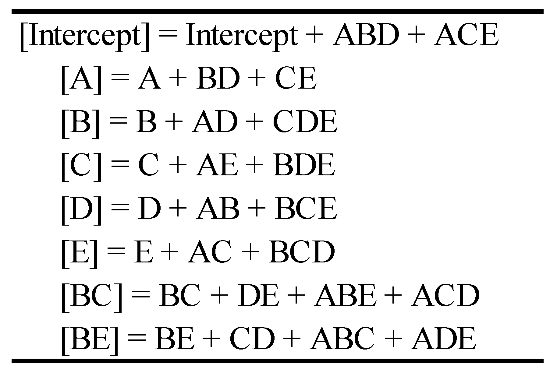
3. Alias Structures for Mixed-Level Designs

This paper explores the use of Pearson’s correlation coefficient and the correlation matrix to construct alias structures for mixed-level designs. This algorithm can be viewed as an alternative to more complex methods, and the resulting alias structures resemble those commonly used for two-level designs. These structures allow the user to visualize the existing correlations among the different terms in the design, especially the main effects and low order interactions. In addition, this method can be effectively used in choosing subsequent runs in a sequential experimentation approach. The terms most highly correlated in the base design can be the focus for the additional runs to best separate these terms. The fractions considered for computing the alias structures are the EAs developed in [2]. The method consists of four simple steps, as displayed in Figure 3.

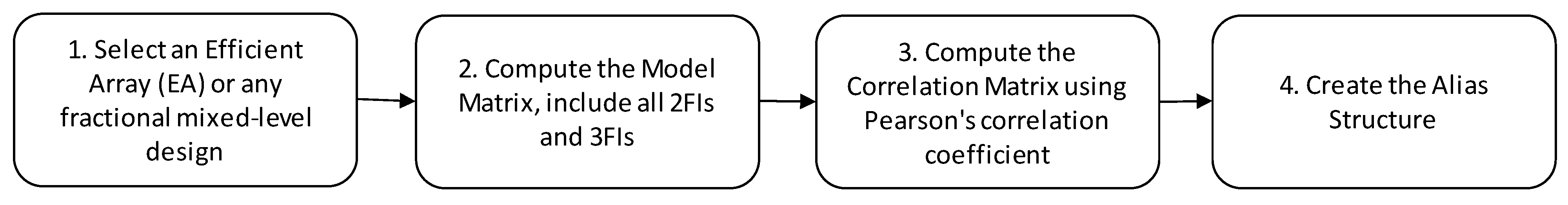
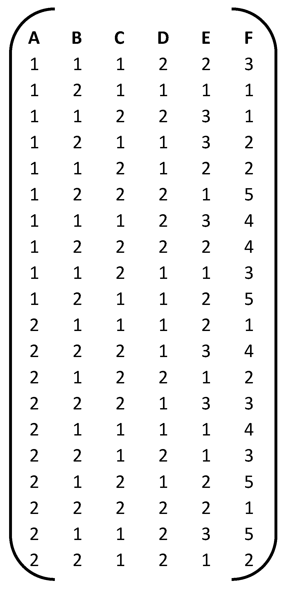
3.1. Initial Design Construction Using EAs

The first step consists of selecting a fractional mixed-level design. This fraction can be constructed by any method, but we will make use of the EAs developed in [2]. Consider, for example, the EA (15, 31 51 71) described in Figure 4, containing 15 runs and 3 factors with 3, 5, and 7 levels, respectively.

3.2. Compute the Model Matrix

The model matrix contains the main effect and interaction columns. Interactions are computed using the Yates order. For this paper, only interactions of the order 2 and 3 were considered using the sparsity of effects principle. Table 1 shows the model matrix.

3.3. Computing the Correlation Matrix Using Pearson’s Correlation Coefficient

Once the model matrix is generated, the next step is to compute all the existing correlations in the design: among the main effects, between main effects and interactions, and among interactions. The Pearson’s correlation coefficient (Equation (1)) was used to compute these correlations. The correlation matrix for the EA (15, 31 51 71) is shown in Table 2.
r j k = C o v ( X j , X k ) v a r X j v a r X k
where, r j k is the Pearson’s correlation coefficient between variables X j and X k , C o v ( X j , X k ) is the covariance between X j and X k , and v a r X j and v a r X k are the variances for variables X j and X k .

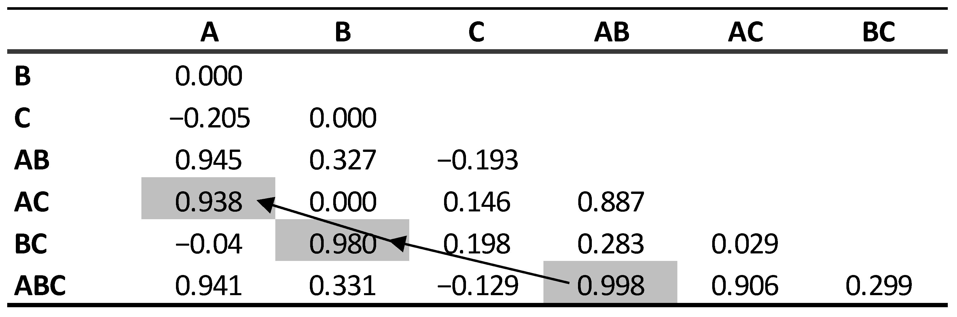
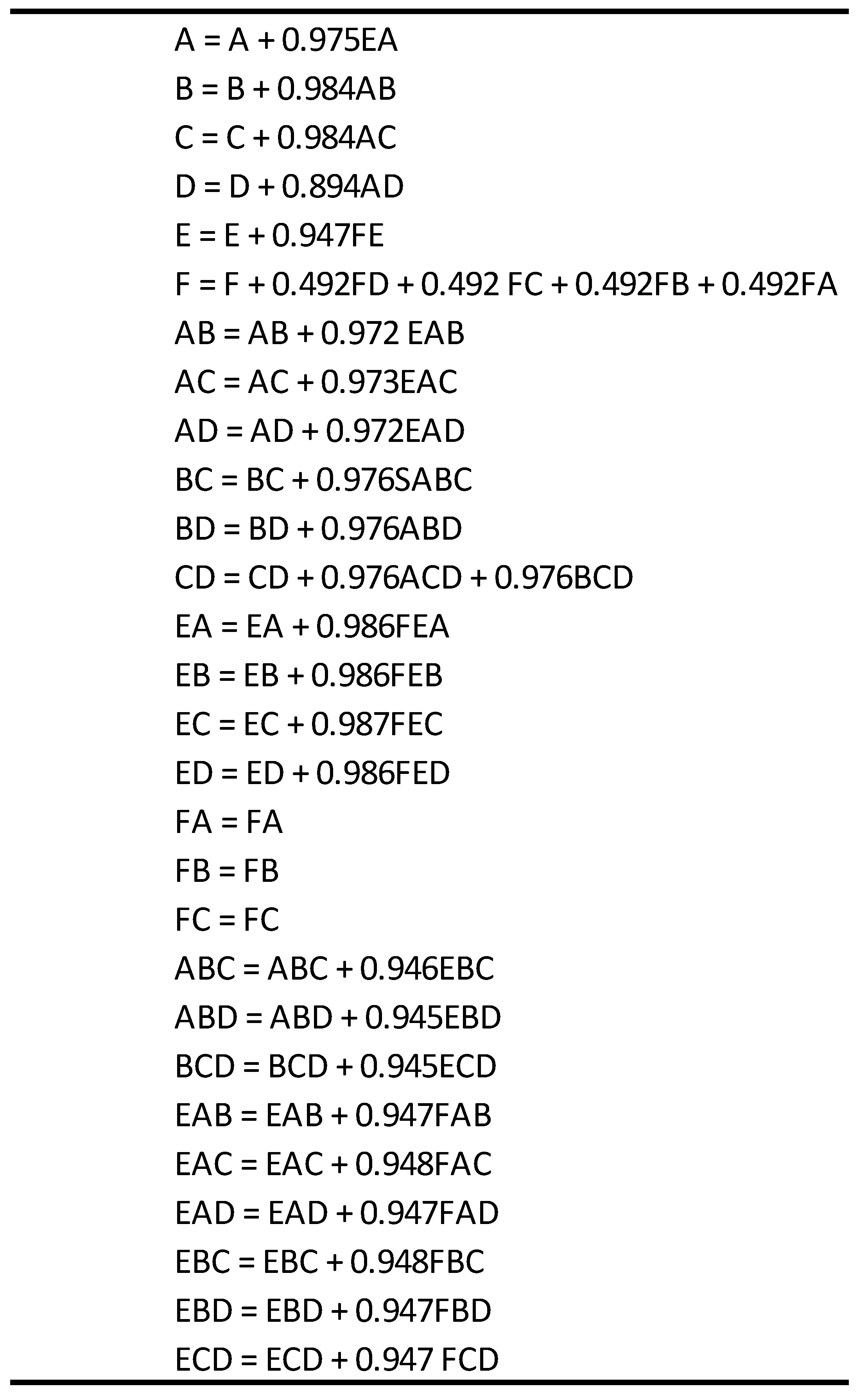
3.4. Creating the Alias Structure

The alias structure can easily be constructed by detecting the highest correlation in the correlation matrix and establishing the relationship between the two terms involved and then, by detecting the next second highest correlation until all terms have been included in an alias chain. The method used to construct the alias structures followed these principles:
  • All main effects and interactions must belong to some chain.
  • The same term cannot be included in multiple alias chains.
  • Lower-order terms are considered more important than higher order terms and should appear sequentially first in the alias chain.
  • Correlations take on values in the interval [−1, 1], and a value of 0 indicates no correlation (orthogonality).
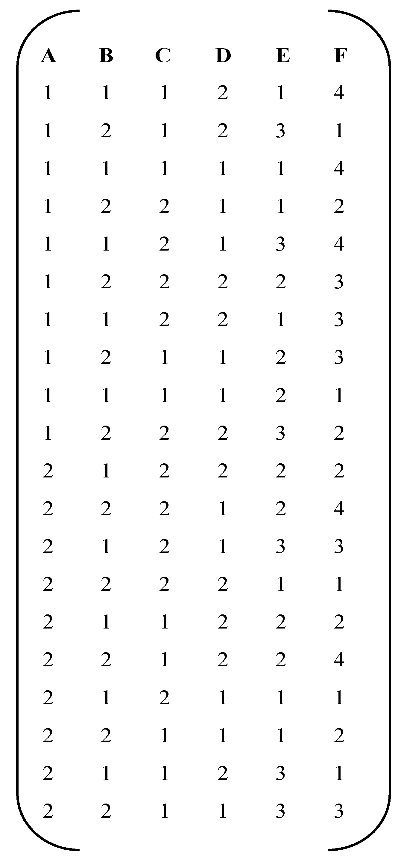
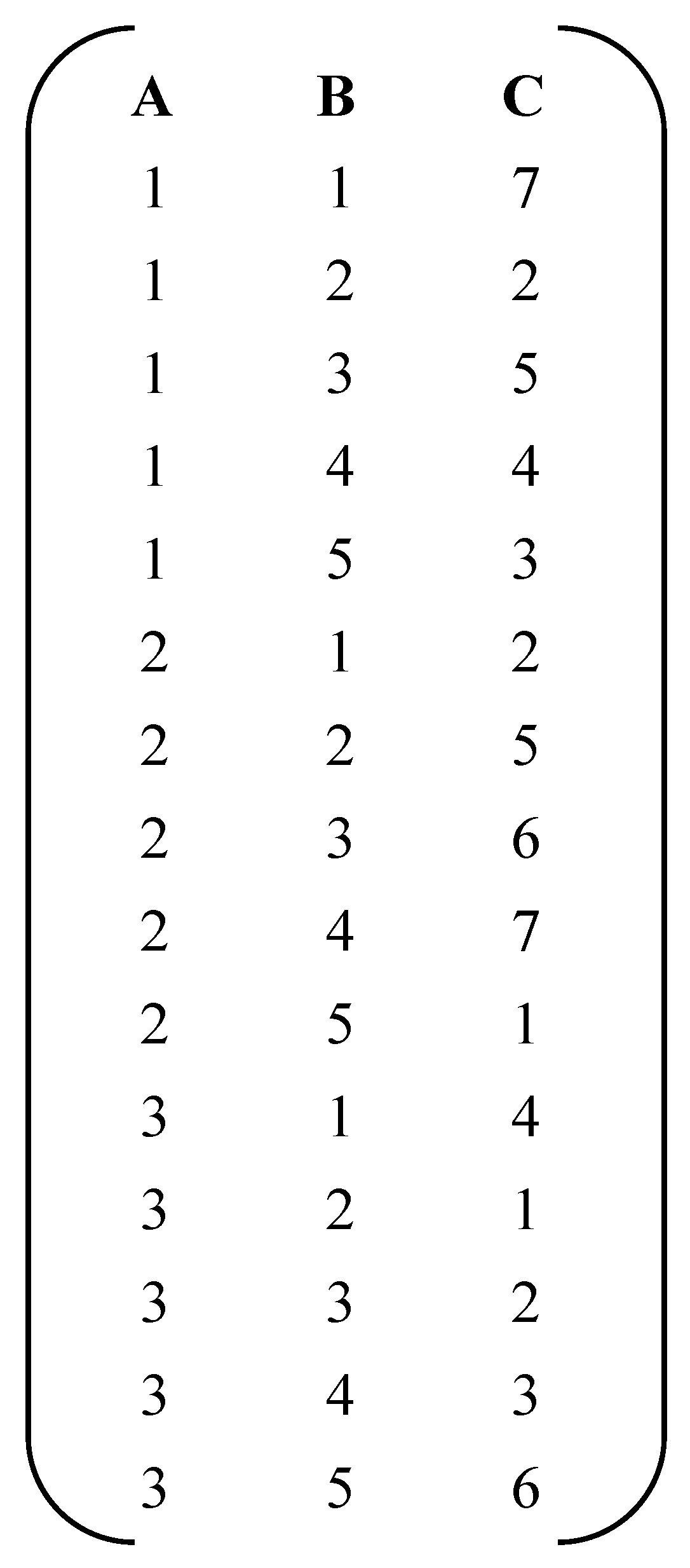
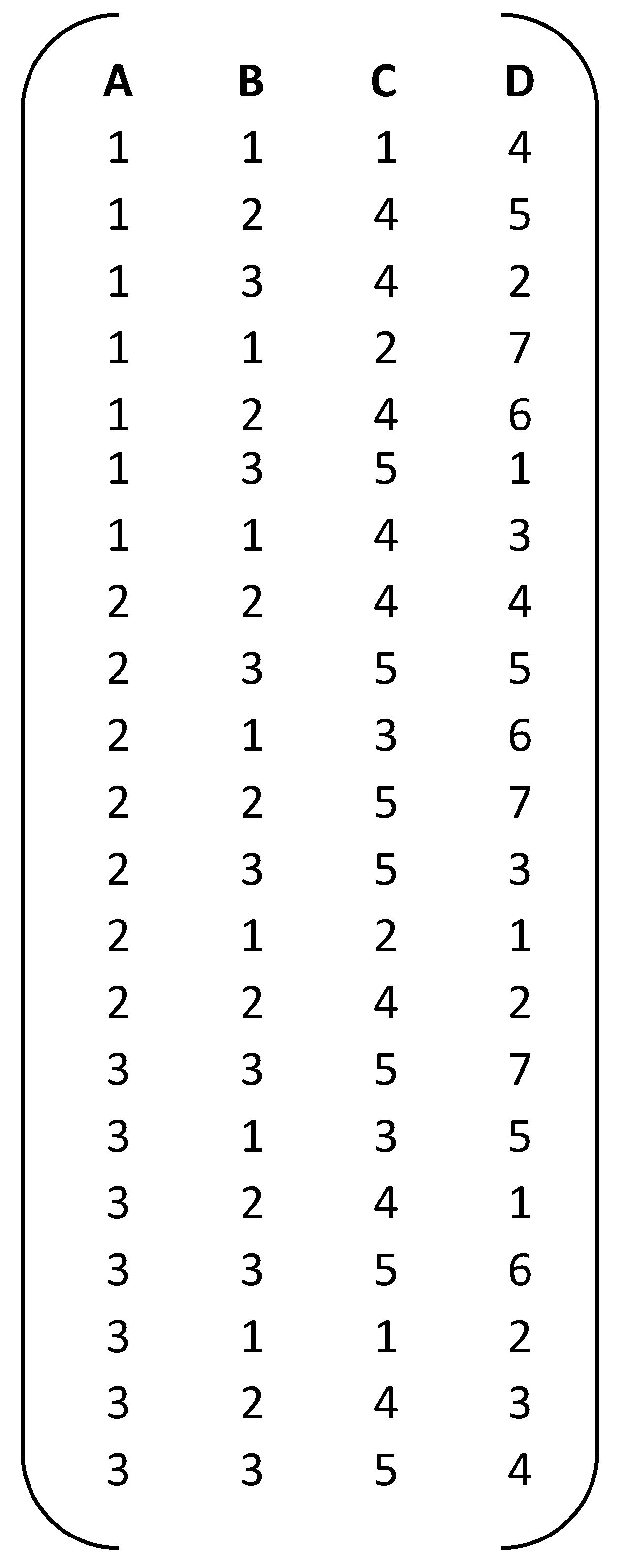
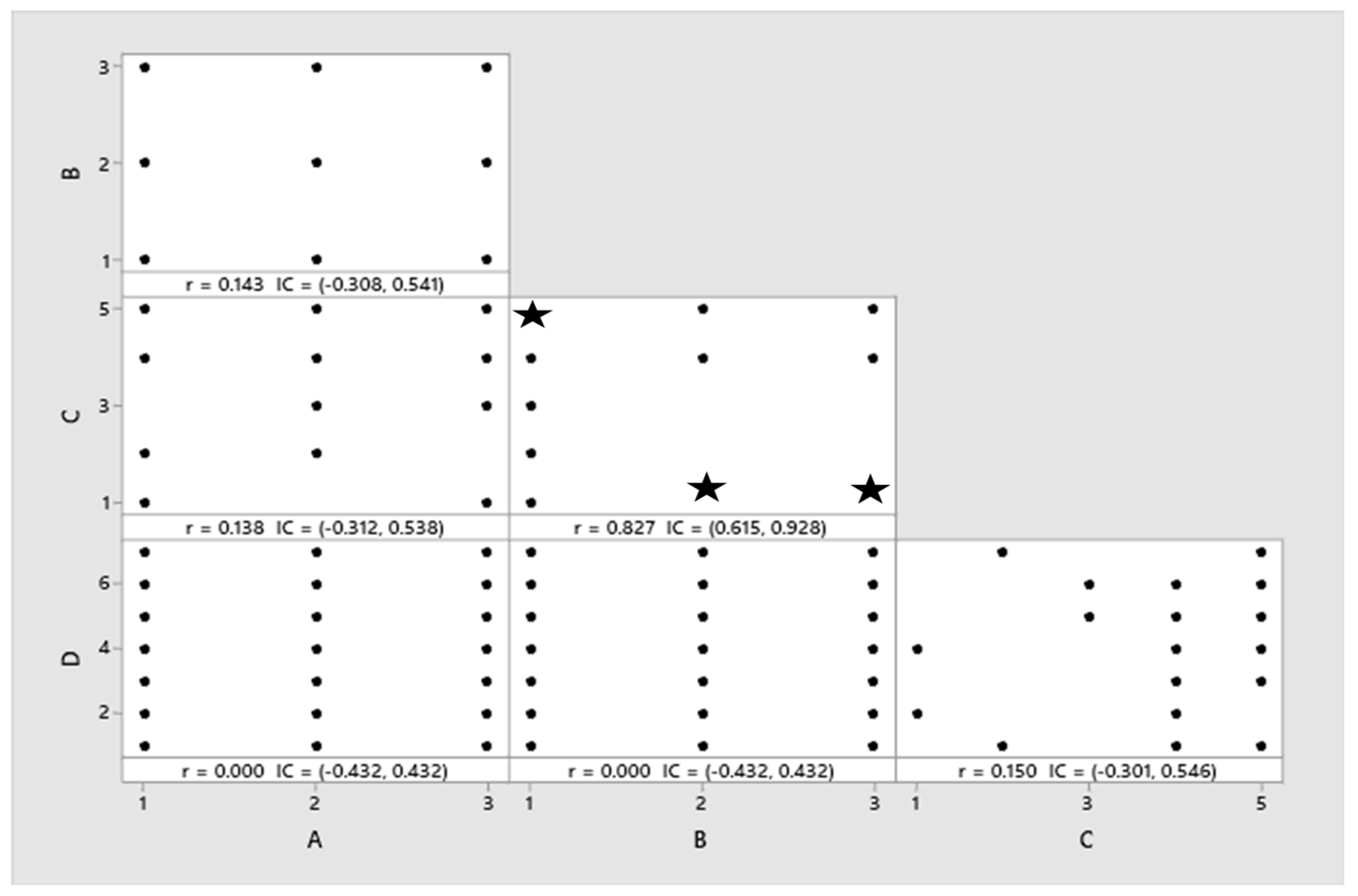
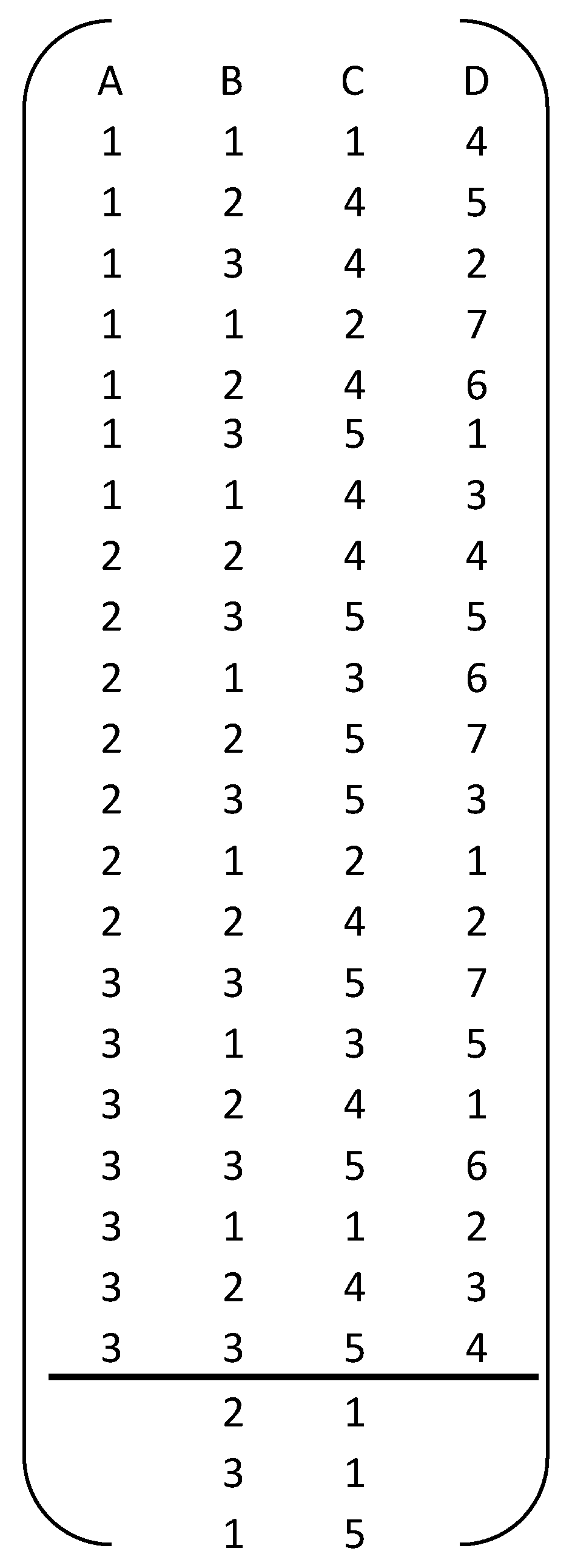
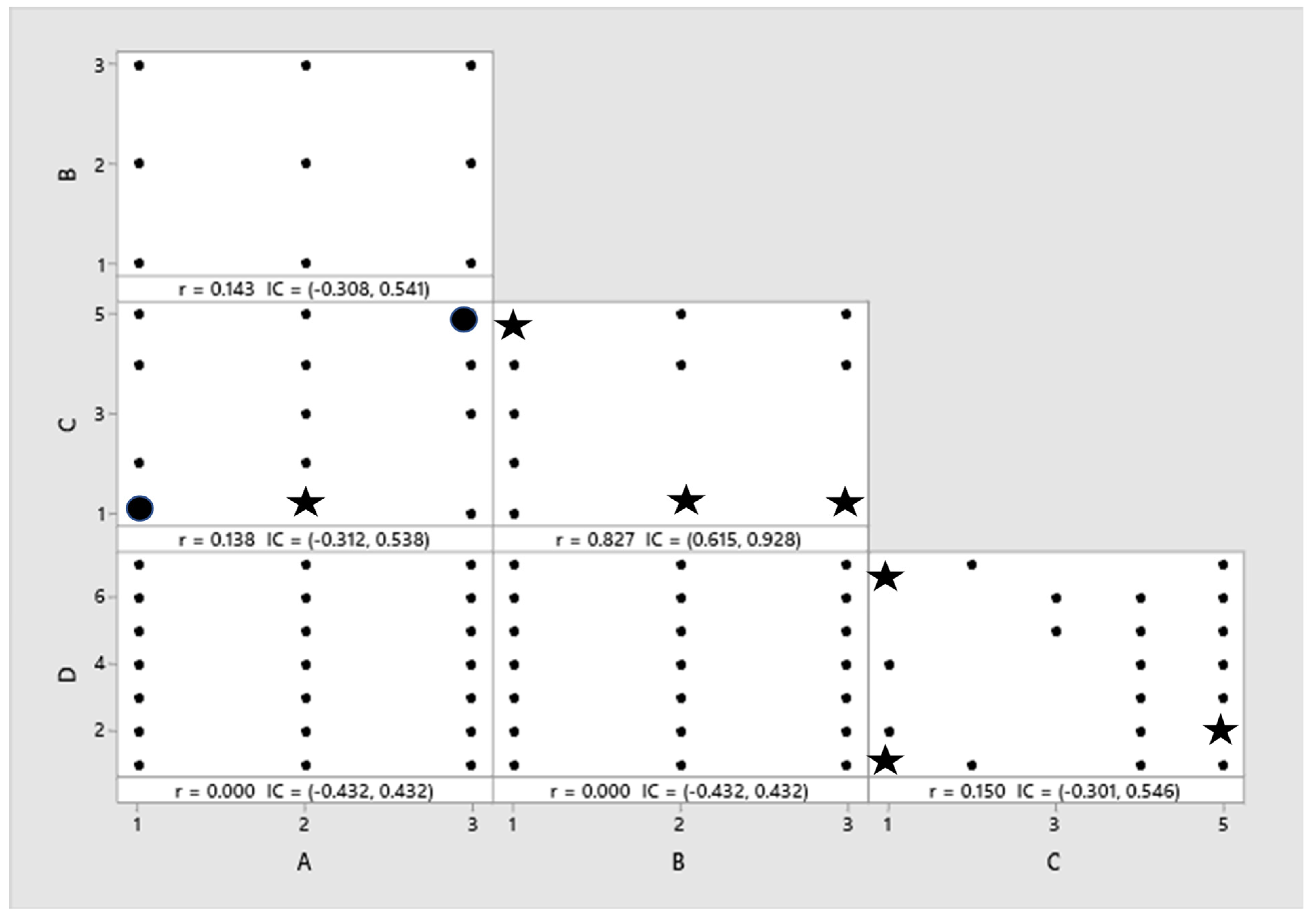
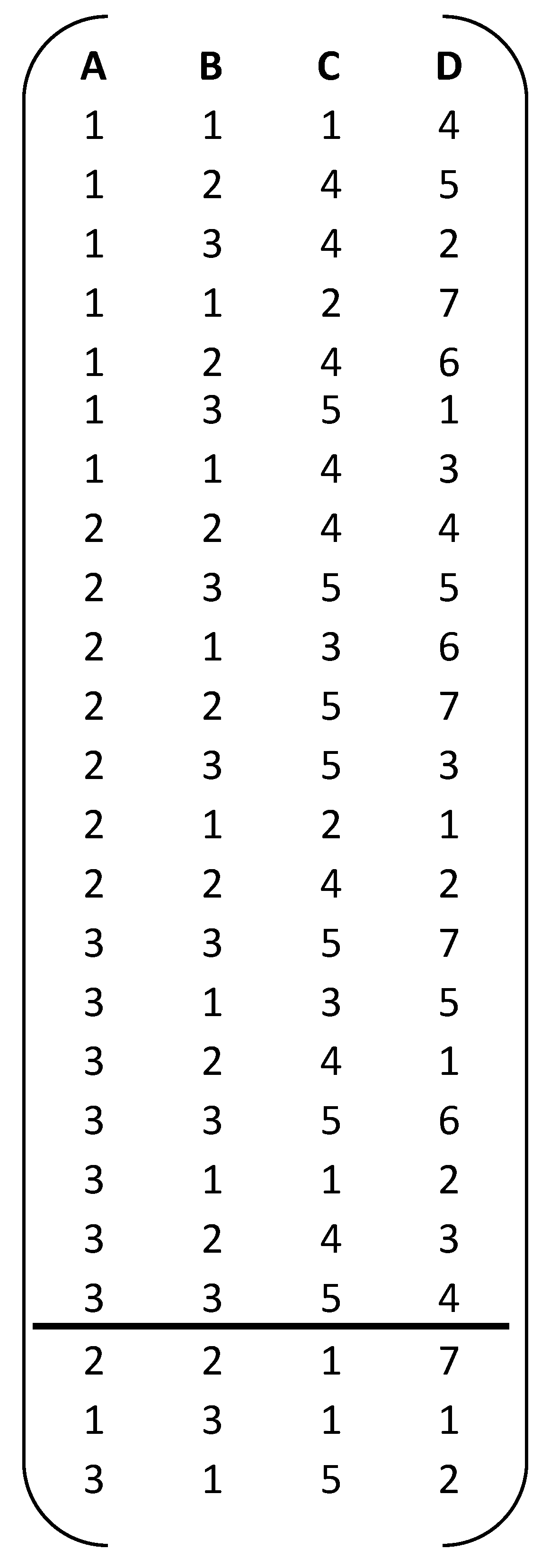
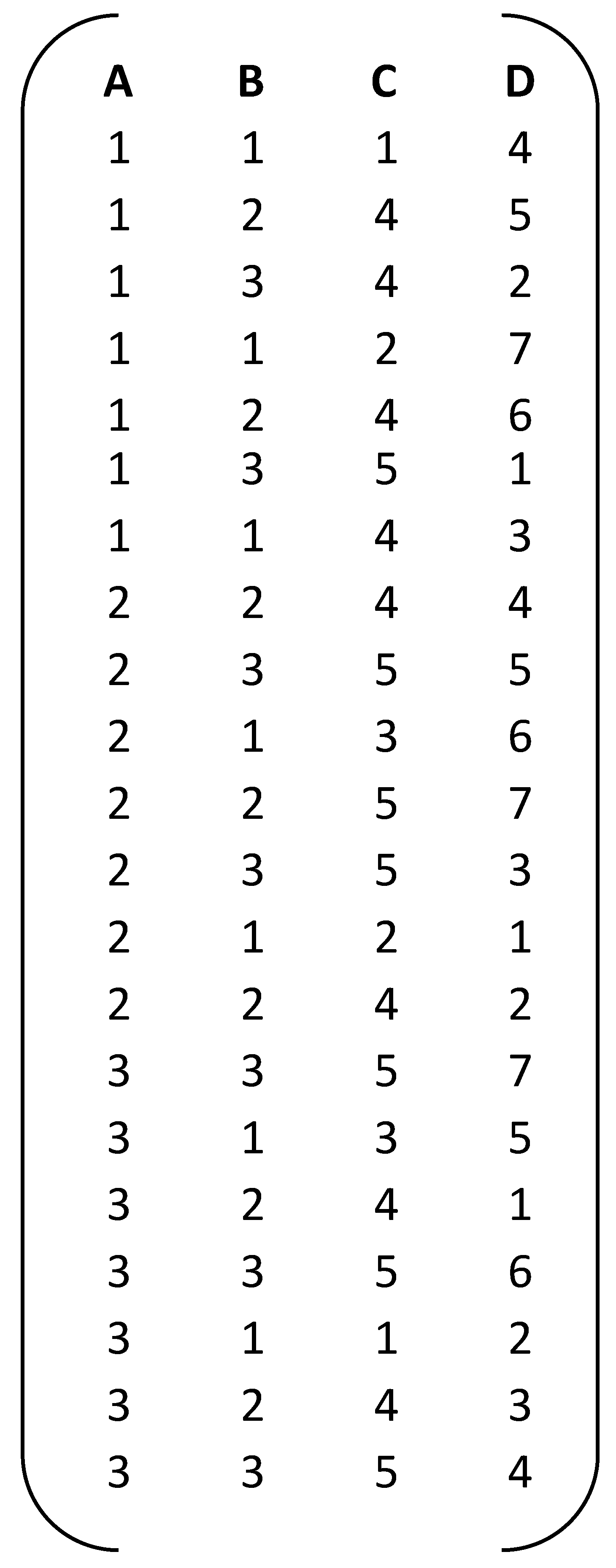
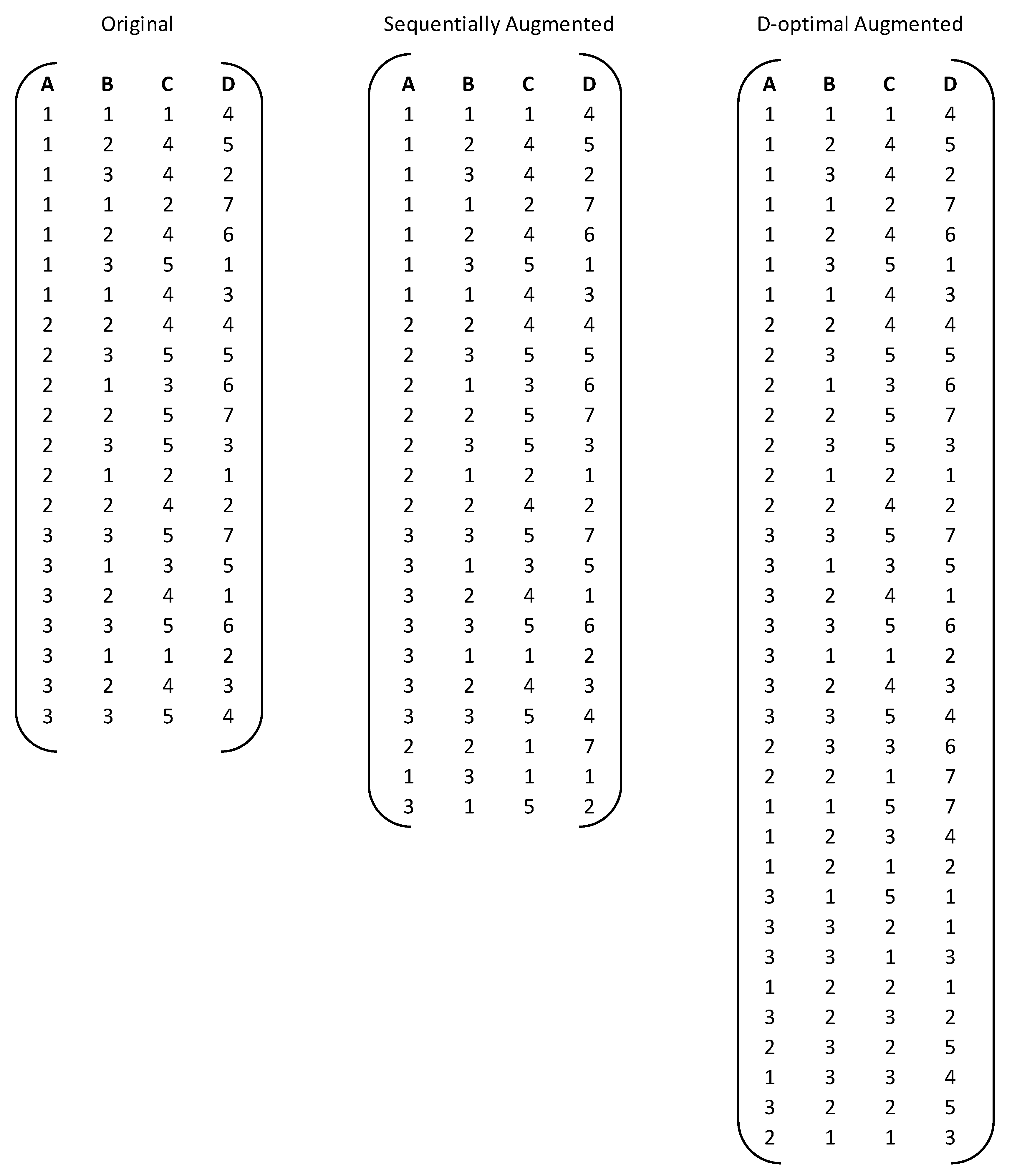
Consider the correlations in Table 2. The highest correlation corresponds to AB and ABC with a value of 0.998. So, the first relation we can establish is
[AB] = AB + 0.998ABC
After this step, AB and ABC are removed from consideration and the next highest correlation corresponds to B and BC with 0.980. The alias structure is augmented with a new chain, resulting in
[B] = B + 0.980BC
[AB] = AB + 0.998ABC
After B and BC are removed, the third highest correlation is between A and AC with 0.938. Therefore, a new chain is added to give
[A] = A + 0.938AC
[B] = B + 0.980BC
[AB] = AB + 0.998ABC
At this point, all effects are included in some chain, except Factor C, so C is added as a chain with no aliases. Figure 5 shows the path followed to construct the alias structure.
[A] = A + 0.938AC
[A] = A + 0.938AC
[B] = B + 0.980BC
[C] = C
[AB] = AB + 0.998ABC
In complex alias situations, effects may appear in separate alias chains, but this makes the alias structure even more complex and confusing. For simplicity, it was decided that each term should appear in only one chain so that only the highest and most important correlations were included in the alias structure. This procedure was tested with several designs, and empirical evidence showed that it was able to create alias structures that properly represented the aliasing in the mixed-level fraction.

4. Example

Consider the EA (20, 24 31 51) shown in Figure 6. Table 3 shows the model matrix containing the main effects, the 2fis and the 3fis. The correlation matrix is shown in Table 4, while the alias structure is displayed in Figure 7 (dots are used to indicate continuation).

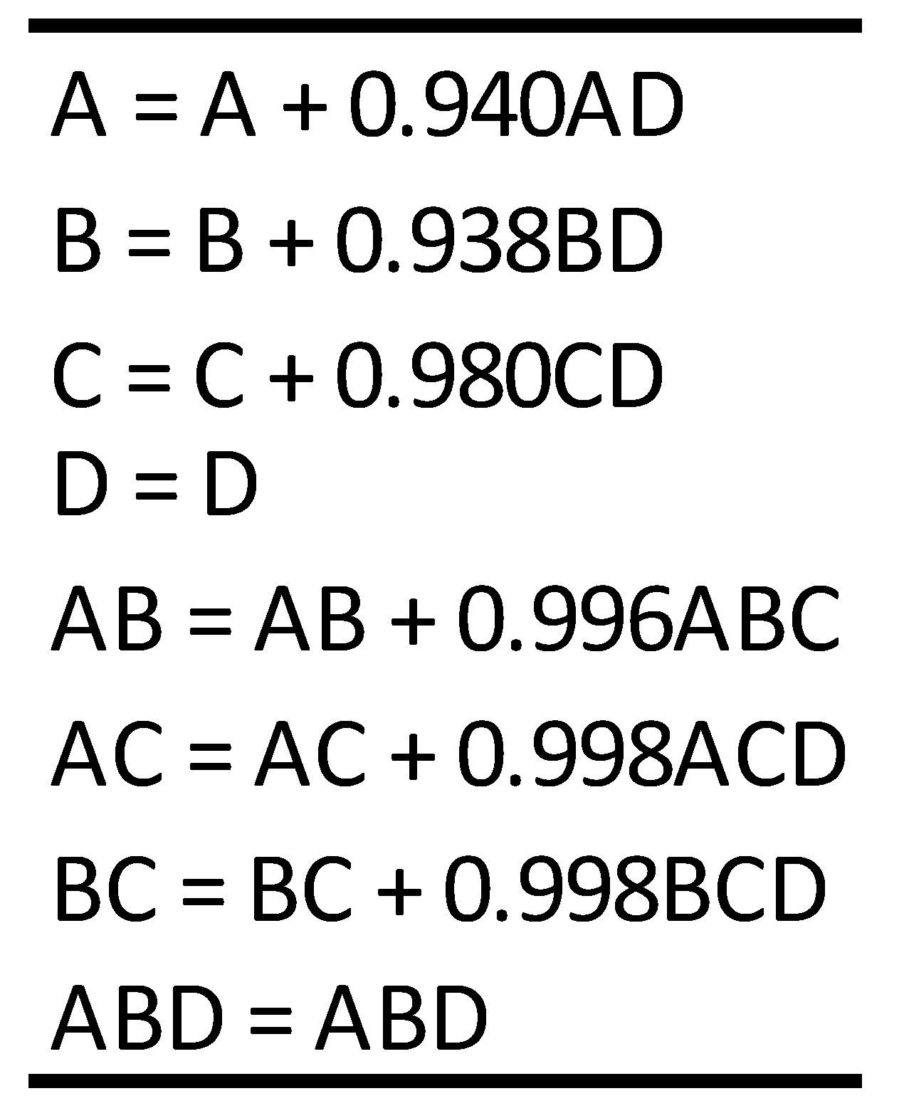
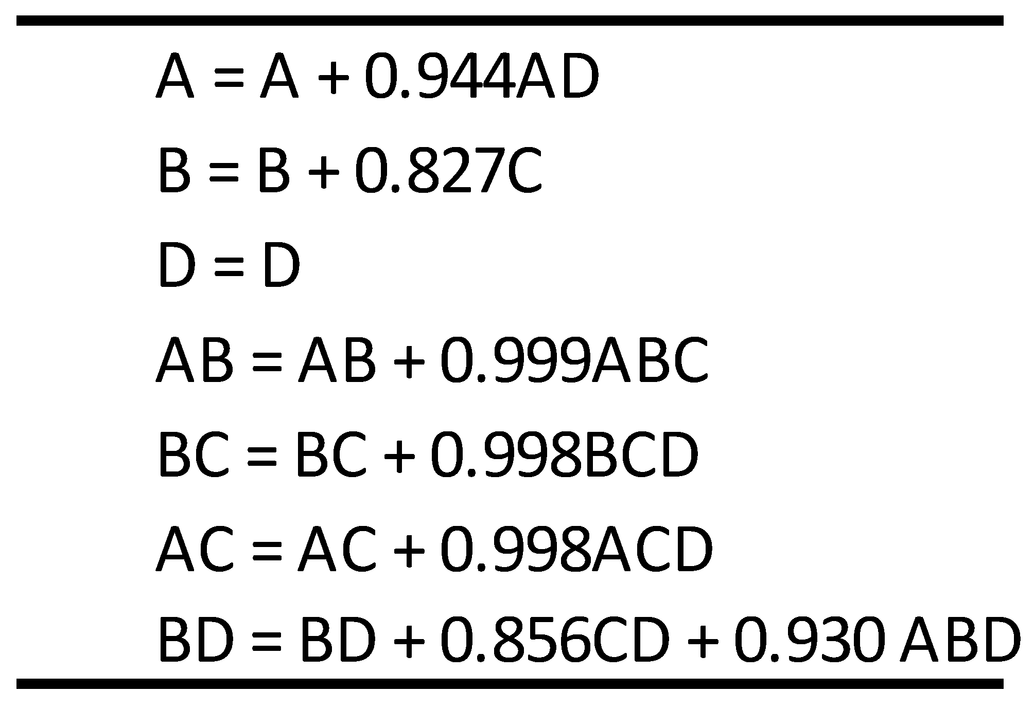
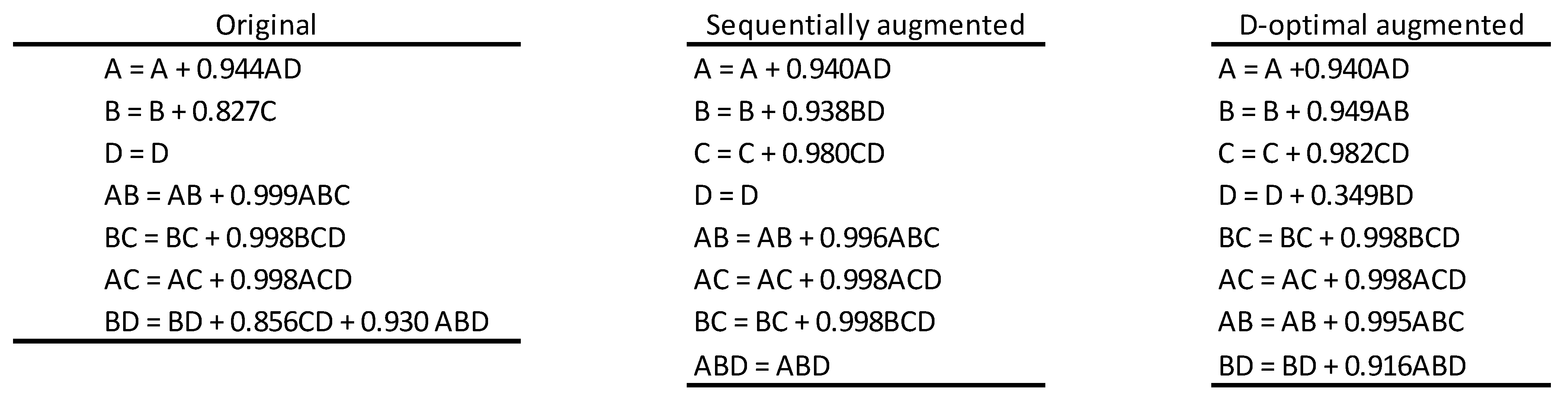
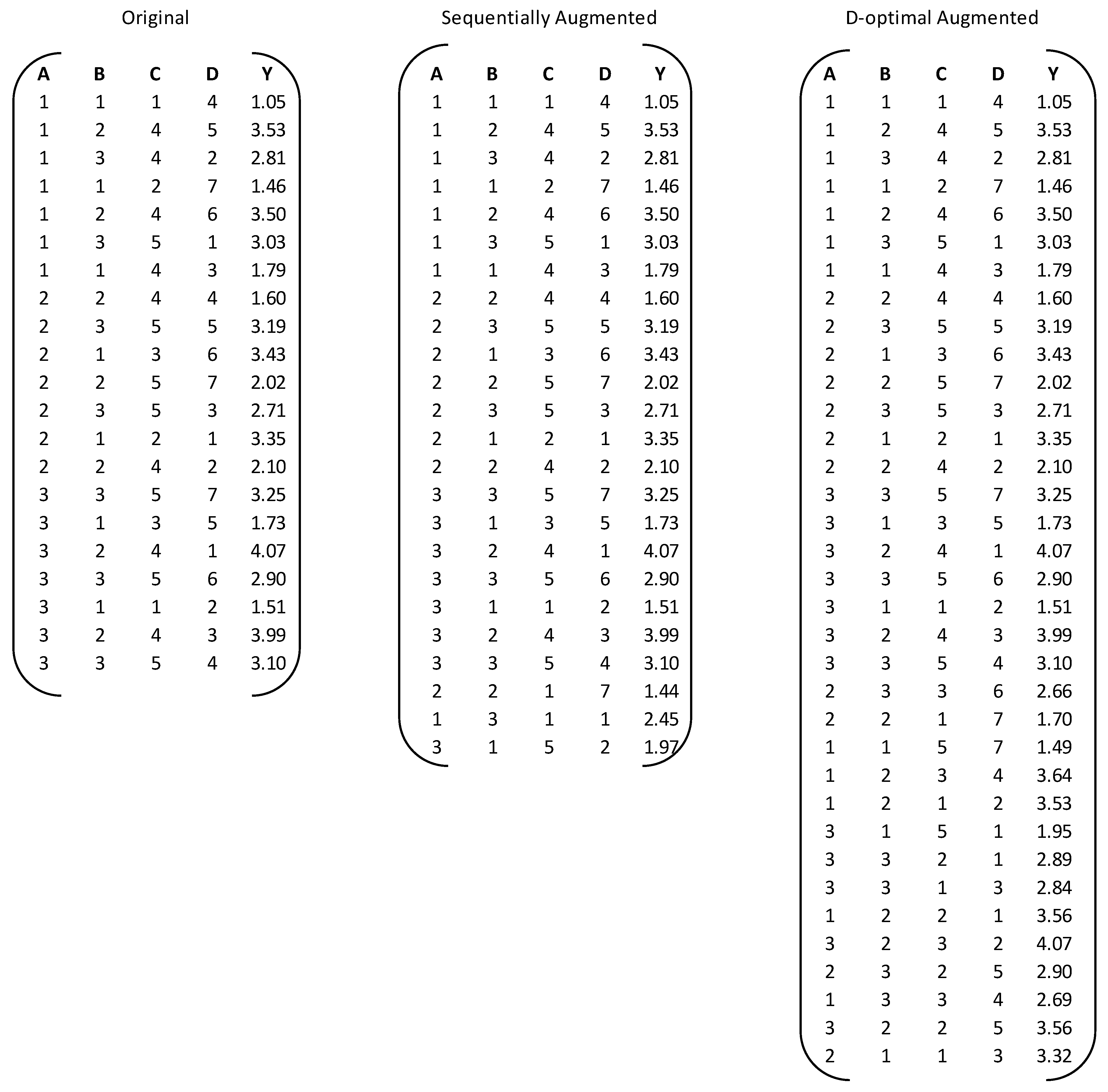
5. Sequential Experimentation Algorithm for Mixed-Level Fractions

The proposed alias structures can be helpful for visualizing the existing correlations in the design and can then be used to break correlations. For example, consider a design where two terms are highly correlated. Runs can be added to reduce the correlation and effectively separate these terms. This approach suggests that sequential experimentation, for mixed-level designs focused on decoupling specific alias chains, is possible. As previously noted, sequential experimentation techniques for mixed-level designs include the fold-over and semifold, which are effective when many or several terms are correlated. In cases in which only a few terms need to be decoupled, adding a small number of runs designed to decouple specific terms can be more efficient. Consider the EA (21, 32 51 71) shown in Figure 8. The alias structure is presented in Figure 9.
Note that the alias structure indicates that factors B and C are strongly correlated. The correlation plot (Figure 10) shows that one way of breaking this correlation is by adding additional runs (2,1), (3,1) and (1,5) for B and C respectively. These runs are indicated by stars. The resulting yet incomplete design is shown in Figure 11.
Signs for A can be added, according to Figure 12. Stars are used to reduce correlation, note that the correlation between A and C can be reduced by adding (2,1) for factors A and C, while the remaining levels of 1 and 3 in Column A (indicated by circles) are chosen to maintain balance in column A. Regarding Column D, levels 7, 1, and 2 can be chosen to create more orthogonality with factor C; these runs become (1,7), (1,1), and (5,2) for C and D, respectively.
The augmented design and its alias structure are shown in Figure 13 and Figure 14, respectively. Note that, after augmentation, Factors B and C are no longer correlated. The procedure shown here has the potential of generating important saving in runs. A fold-over produces a design with 42 runs, and a semifold requires 30 runs. When compared to a fold-over and semifold, this 24-run alternative is obviously more efficient. The next section presents a practical application in which the algorithm, presented here, is compared to D-optimal augmentation.
The sequential augmentation algorithm for mixed-level fractions, presented here, can be summarized in the next steps.
  • Use the alias structure and the correlation plot to detect the highest correlation.
  • Add new runs to achieve orthogonality.
  • Determine signs for remaining factors in such a way that balance is maintained.
  • Compute the new alias structure and correlation plot.
  • Repeat the procedure if necessary.

6. Practical Applications

Consider the poultry industry and, in particular, chicken rearing. Let us assume that four factors are involved in this process: (A) 3 chicken breeds, (B) 3 breeding places, (C) 5 hormones, (D) 7 food formulas. This is a 32 51 71 mixed-level design, and the full factorial consists of 315 runs. The experimenter is interested in running a fraction. Consider the EA (21, 32 51 71), shown in Figure 15, and its alias structure shown in Figure 16.
The alias structure shows that two main effects, B and C are strongly correlated. This means that this design will have difficulty estimating main effects. If this design is selected, model construction and optimization could be poor.
The experimenter is interested in augmenting the design to break the correlation between factors B and C, and two options are available: the sequential augmentation algorithm, presented in Section 6, and the D-optimal augmentation. Figure 17 shows the original, sequentially augmented, and D-optimal augmented designs, and Figure 18 shows the corresponding alias structures, Moreover, it shows that the sequentially augmented and D-optimal augmented designs can estimate all main effects, apart from each other, because they belong to different alias chains. These designs have no problem estimating the correct model and optimizing the process. On the other hand, the original design was not able to estimate factor C, which means that the correct model will not be estimated, and the optimization process will not be as good as that of the other two designs. To prove this, a Monte Carlo simulation was performed. Figure 19 shows the simulated data for the three designs generated in such a way that effects of A, B, and C, and the interaction AB, should be reported as significant. A low noise level was employed.
Table 5 presents the significant terms detected by each design. Note that the original design EA (21, 32 51 71) was not able to identify the significant effect C; it only detected factors A, B, and interaction AB as significant. On the other hand, the sequentially augmented and D-optimal augmented designs were able to identify all significant effects A, B, C, plus the interaction AB. The analysis was performed using Design Expert software. Table 6 shows the optimization; the asterisk * indicates that the factor was reported as not significant. Note that the EA (21, 32 51 71) produced a chicken that weighs 4.02 pounds, while the other two designs produced a chicken that weighs 4.14 and 4.05 pound, respectively. This difference may not seem significant, but on an industrial level, it could be a competitive advantage.
To construct mixed-level fractions, we recommended the approach proposed by [34,35] to produce a near orthogonal balanced design. To achieve more orthogonality, we recommended the use of the sequential experimentation algorithm, presented in Section 5, or D-optimal augmentation. The sequential experimentation algorithm is useful in cases where only a few terms needed to be decoupled. It can be used to generate significant savings in runs, given that the D-optimal augmentation technique is usually more expensive. We do not recommend the use of foldovers or semifolds, given that these techniques require computer programming and complex search methods, such as genetic algorithms and exhaustive searches, and they may not be the best option for most practitioners.

7. Computer Program

A code for the construction of alias structures was developed in Matlab software because it has a large number of strategies for the efficient use of memory, in which large matrices can be used and stored. For example, for a 9-factor design with 36 runs, the capacity used by the matrices, generated by the program, is 673 MB with a correlation matrix of size 92 × 92. Therefore, for a computer with a capacity of 8 GB, the maximum memory available for these arrays would be 2643 MB. Note that this will be limited by the available system memory (physical + swap file). Capacity is not a problem in the current structure of the code. The correlation matrix is calculated and then stored in an array, thus allowing this information to be used in subsequent calculations. A portion of the programming code is shown below (Algorithm 1). The full code is available at Supplementary Materials Section.
Algorithm 1. Program Alias
function [ ALIASESTRUCTURE ] = GENERADORESTRUCTURAALIASITC(FRACTION)
Array=FRACTION;
ponderacion=0.5;
[m,n]=size(Array);
matrizdecorrelaciones=PASO1A3CALCULARCORRELACIONES(Array,n);
PASO4;
ijcontador=0;
for columname=1:me-1
   columname;
   contador=columname+1;
     for filame=contador:me
       if ijcontador==1
              break
       end
       valor=W(filame,columname);
          if abs(valor)>=1.5
          ijcontador=ijcontador+1;
          disp(’La fracción contiene efectos principales que estan fuertemente correlacionados (r>0.5)’ )
          end
          contador=contador+1;
     end
 if ijcontador==1
 break
 end
 end
 ciclo=1;
 while ciclo==1
  if ijcontador==0
   PASO5
   else
  break
   end
end
end
The MATLAB program significantly reduced the time invested in the construction of alias structures for mixed-level fractional factorial designs. Figure 20 shows the computational time required by the program, which ran on a computer with an AMD E-450 processor and a RAM of 2 GB. Building structures for a 9-factor mixed-level fractional design using the program took only 2 s. The program also reduced the uncertainty of calculations and interpretive errors that commonly appear when alias structures are built manually.

8. Conclusions

The method to construct alias structures for fractional mixed-level designs, presented in this paper, is simple and easy to implement. It can be summarized in four steps: (1) select an efficient array; (2) compute the model matrix; (3) compute the correlation matrix; (4) construct the alias structure. The construction method selects the highest correlations and establishes relationships among columns until all terms of interest (main effects and interactions) have been included in some alias chain.
Alias structures serve as the basis for a sequential experimentation approach. A new algorithm, focused on separating specific columns for main effects, is proposed. The algorithm is applied to a practical case and compared to D-optimal augmentation. The results show that, in cases when only a few terms need to be decoupled, the sequential augmentation algorithm tends to be more efficient than D-optimal augmentation.
The conclusion is that alias structures for mixed-level designs can be easily constructed, help to visualize the existing correlation in the design, and constitute a good complement to the GBM criterion. In addition, the sequential augmentation algorithm is able to decouple specific terms while using a small number of runs.

Supplementary Materials

The full code of the program for generating alias structures and instructions of use are available at: https://0-www-mdpi-com.brum.beds.ac.uk/article/10.3390/math9233053/s1.

Author Contributions

Conceptualization, A.J.R.-L.; methodology, A.J.R.-L.; software, Y.V.P.-P.; validation, J.A.V.-L.; formal analysis, Y.V.P.-P. and J.A.J.-G.; investigation, A.J.R.-L. and Y.V.P.-P.; resources, M.T.-E.; writing—original draft preparation, M.L.A.-E.; writing—review and editing, A.J.R.-L. and Y.V.P.-P.; supervision, A.J.R.-L. and Y.V.P.-P.; project administration, A.J.R.-L. All authors have read and agreed to the published version of the manuscript.

Funding

This research received no external funding.

Data Availability Statement

Not applicable.

Conflicts of Interest

The authors declare no conflict of interest.

References

  1. Montgomery, D.C. Design and Analysis of Experiments, 9th ed.; Wiley and Sons Inc.: Hoboken, NJ, USA, 2017. [Google Scholar]
  2. Guo, Y.; Simpson, J.R.; Pignatiello, J.J. Construction of Efficient Mixed-Level Fractional Factorial Designs. J. Qual. Technol. 2007, 39, 241–257. [Google Scholar] [CrossRef]
  3. Wang, J.C.; Wu, C.F.J. An Approach to the Construction of Asymmetrical Orthogonal Arrays. J. Am. Stat. Assoc. 1991, 86, 450. [Google Scholar] [CrossRef]
  4. DeCock, D.; Stufken, J. On finding mixed orthogonal arrays of strength 2 with many 2-level factors. Stat. Probab. Lett. 2000, 50, 383–388. [Google Scholar] [CrossRef]
  5. Xu, H. An Algorithm for Constructing Orthogonal and Nearly-Orthogonal Arrays with Mixed Levels and Small Runs. Technometrics 2002, 44, 356–368. [Google Scholar] [CrossRef] [Green Version]
  6. Koukouvinos, C.; Mantas, P. Construction of some E(fNOD) optimal mixed-level supersaturated designs. Stat. Probab. Lett. 2005, 74, 312–321. [Google Scholar] [CrossRef]
  7. Fang, K.-T.; Lin, D.K.J.; Liu, M.-Q. Optimal mixed-level supersaturated design. Metrika 2003, 58, 279–291. [Google Scholar] [CrossRef]
  8. Yan, L.; Min-Qian, L. Construction of optimal supersaturated design with large number of levels. J. Stat. Plan. Inference 2011, 141, 2035–4043. [Google Scholar]
  9. Sun, F.; Lin, D.K.J.; Liu, M.-Q. On construction of optimal mixed-level supersaturated designs. Ann. Stat. 2011, 39, 197–211. [Google Scholar] [CrossRef]
  10. Yamada, S.; Lin, D.K. Three-level supersaturated designs. Stat. Probab. Lett. 1999, 45, 31–39. [Google Scholar] [CrossRef]
  11. Guo, Y.; Simpson, J.R.; Pignatiello, J.J., Jr. The general balance metric for mixed-level fractional factorial designs. Qual. Reliab. Eng. Int. 2009, 25, 335–344. [Google Scholar] [CrossRef]
  12. Wu, C.F.; Hamada, M. Experiments: Planning, Analysis and Parameters Desing Optimization; Wiley & Sons: Hoboken, NJ, USA, 2009. [Google Scholar]
  13. Mukerjee, R.; Wu, C.F. A Modern Theory of Factorial Design; Springer: New York, NY, USA, 2006. [Google Scholar]
  14. Pistone, G.; Rogantin, M.-P. Indicator function and complex coding for mixed fractional factorial designs. J. Stat. Plan. Inference 2008, 138, 787–802. [Google Scholar] [CrossRef] [Green Version]
  15. Grömping, U.; Xu, H. Generalized resolution for orthogonal arrays. Ann. Stat. 2014, 42, 918–939. [Google Scholar] [CrossRef] [Green Version]
  16. Guo, Y.; Simpson, J.R.; Pignatiello, J.J., Jr. Optimal foldover plans for mixed-level fractional factorial designs. Qual. Reliab. Eng. Int. 2009, 25, 449–466. [Google Scholar] [CrossRef]
  17. Ríos, A.J.; Simpson, J.R.; Guo, Y. Semifold plans for mixed-level designs. Qual. Reliab. Eng. Int. 2011, 27, 921–929. [Google Scholar] [CrossRef]
  18. Box, G.E.; Hunter, J.S. The 2kp Fractional Factorial Designs. Technometrics 1961, 3, 311–351. [Google Scholar] [CrossRef]
  19. Su, H.; Wu, C.F.J. CME Analysis: A New Method for Unraveling Aliased Effects in Two-Level Fractional Factorial Experiments. J. Qual. Technol. 2017, 49, 1–10. [Google Scholar] [CrossRef]
  20. Xu, H. Nonregular Factorial and Supersaturated Designs. In Handbook of Design and Analysis of Experiments; Dean, A., Morris, M., Stufken, J., Bingham, D., Eds.; Taylor & Francis Group: Boca Raton, FL, USA, 2015; pp. 339–367. [Google Scholar]
  21. Kulahci, M.; Bisgaard, S. A generalization of the alias matrix. J. Appl. Stat. 2006, 33, 387–395. [Google Scholar] [CrossRef]
  22. Jones, B.; Montgomery, D.C. Alternatives to resolution IV screening designs in 16 runs. Int. J. Exp. Des. Process. Optim. 2010, 1, 285. [Google Scholar] [CrossRef]
  23. Al-Ghamdi, K.A. Improving the Practice of Experimental Design in Manufacturing Engineering. Ph.D. Thesis, University of Birmingham, Birmingham, AL, USA, 2011. [Google Scholar]
  24. Hamada, M.; Wu, C.F.J. Analysis of Designed Experiments with Complex Aliasing. J. Qual. Technol. 1992, 24, 130–137. [Google Scholar] [CrossRef]
  25. Hamada, C.A.; Hamada, M.S. All-subsets regression under effect heredity restrictions for experimental designs with complex aliasing. Qual. Reliab. Eng. Int. 2010, 26, 75–81. [Google Scholar] [CrossRef]
  26. Wu, H.; Mee, R.; Tang, B. Fractional Factorial Designs with Admissible Sets of Clear Two-Factor Interactions. Technometrics 2012, 54, 191–197. [Google Scholar] [CrossRef] [Green Version]
  27. Tsai, P.-W.; Gilmour, S.G. A General Criterion for Factorial Designs Under Model Uncertainty. Technometrics 2010, 52, 231–242. [Google Scholar] [CrossRef]
  28. Cheng, C.-S.; Tsai, P.-W. Multistratum fractional factorial designs. Stat. Sin. 2011, 21, 1001–1021. [Google Scholar] [CrossRef] [Green Version]
  29. Cheng, C.-S.; Tsai, P.-W. Templates for design key construction. Stat. Sin. 2014, 23, 1419–1436. [Google Scholar] [CrossRef]
  30. Zhou, Q.; Balakrishnan, N.; Zhang, R. The factor aliased effect number pattern and its application in experimental planning. Can. J. Stat. 2013, 41, 540–555. [Google Scholar] [CrossRef]
  31. Tyssedal, J.; Niemi, R. Graphical Aids for the Analysis of Two-Level Nonregular Designs. J. Comput. Graph. Stat. 2014, 23, 678–699. [Google Scholar] [CrossRef]
  32. Sartono, B.; Goos, P.; Schoen, E. Constructing General Orthogonal Fractional Factorial Split-Plot Designs. Technometrics 2015, 57, 488–502. [Google Scholar] [CrossRef] [Green Version]
  33. Jones, B.; Nachtsheim, C.J. Efficient Designs with Minimal Aliasing. Technometrics 2011, 53, 62–71. [Google Scholar] [CrossRef]
  34. Pantoja, Y.V.; Ríos, A.J.; Esquivias, M.T. A method for construction of mixed-level fractional designs. Qual. Reliab. Eng. Int. 2019, 35, 1646–1665. [Google Scholar] [CrossRef]
  35. Pantoja-Pacheco, Y.; Ríos-Lira, A.; Vázquez-López, J.; Jiménez-García, J.; Asato-España, M.; Tapia-Esquivias, M. One Note for Fractionation and Increase for Mixed-Level Designs When the Levels Are Not Multiple. Mathematics 2021, 9, 1455. [Google Scholar] [CrossRef]
Figure 1. Efficient Array EA (20, 24 31 41).
Mathematics 09 03053 g001
Figure 2. Alias structure for a 25−2.
Mathematics 09 03053 g002
Figure 3. Method for constructing alias structures for mixed-level designs.
Mathematics 09 03053 g003
Figure 4. EA (15, 31 51 71).
Mathematics 09 03053 g004
Figure 5. Path followed to construct the alias structure.
Mathematics 09 03053 g005
Figure 6. EA (20, 24 31 51).
Mathematics 09 03053 g006
Figure 7. Alias structure for EA (20, 24 31 51).
Mathematics 09 03053 g007
Figure 8. EA (21, 32 51 71).
Mathematics 09 03053 g008
Figure 9. Alias structure for EA (21, 32 51 71).
Mathematics 09 03053 g009
Figure 10. Breaking correlation between B and C.
Mathematics 09 03053 g010
Figure 11. EA (24, 32 51 71) with additional signs for B and C.
Mathematics 09 03053 g011
Figure 12. Assignment of signs for columns A and D.
Mathematics 09 03053 g012
Figure 13. EA (24, 32 51 71).
Mathematics 09 03053 g013
Figure 14. Alias structure for EA (24, 32 51 71).
Mathematics 09 03053 g014
Figure 15. EA (21, 32 51 71).
Mathematics 09 03053 g015
Figure 16. Alias structure for EA (21, 32 51 71).
Mathematics 09 03053 g016
Figure 17. Original, sequentially augmented, and D-optimal augmented designs.
Mathematics 09 03053 g017
Figure 18. Alias structures for original, sequentially augmented, and D-optimal augmented designs.
Mathematics 09 03053 g018
Figure 19. Simulated data for original, sequentially augmented, and D-optimal augmented designs.
Mathematics 09 03053 g019
Figure 20. MATLAB Code computational time.
Mathematics 09 03053 g020
Table 1. Model matrix for EA (15, 31 51 71).
ABCBACACBCBA
1171777
1222299
135351919
144442525
153533131
21269237
2257121247
2368132055
2479142863
2511082964
3141118474
3211215878
33213161686
34314172494
356152034104
Table 2. Correlation matrix for EA (15, 31 51 71).
ABCABACBC
B0.000
C−0.2050.000
AB0.9450.327−0.193
AC0.9380.0000.1460.887
BC−0.0400.9800.1980.2830.029
ABC0.9410.331−0.1290.9980.9060.299
Table 3. Model matrix for EA (20, 24 31 51).
ABCDEFABACADEAFABC...ECDFCDFECFED
111223113231...813823
121111311112...1111
112231133313...12162626
121132311322...321212
112122131223...57227
122215333154...10202020
111234113341...9141429
122224333244...11192424
112113131133...48183
121125311252...251010
211121222561...2166
222134442694...692914
212212244473...10171717
222133442684...682813
211114222491...1444
221213424482...713318
2121252425103...5102510
222221444564...11162121
2112352246101...9151530
221212424472...712217
Table 4. Correlation matrix for EA (20, 24 31 51).
ABCDEFABAC...EBDFBDFEBECDFCDFEC
B0 ...
C00 ...
D000 ...
E−0.06−0.060.062−0.06 ...
F00000.088 ...
AB0.4470.89400−0.080 ...
AC0.44700.89400.02800.2 ...
AD0.447000.894−0.0800.20.2...
EA0.875−0.030.03−0.030.4290.0430.3640.418...
FA0.87000−0.010.4920.3890.389...
BC00.4470.89400.02800.40.8...
BD00.44700.894−0.0800.40...
EB−0.030.8750.03−0.030.4290.0430.7690.013...
FB00.8700−0.010.4920.7780...
CD000.4470.894−0.03000.4...
EC−0.03−0.030.888−0.030.5140.041−0.040.781...
FC000.8700.0970.49200.778...
ED−0.03−0.030.030.8750.4290.043−0.040.013...
FD0000.87−0.010.49200...
FE−0.06−0.060.057−0.060.9470.404−0.080.026...
ABC0.2180.4360.87300.01400.4880.878...
ABD0.2180.43600.873−0.100.4880.098...
EAB0.4290.8720.015−0.020.1550.0210.9720.205...
FAB0.4340.86700−0.060.2450.9690.194...
ACD0.21800.4360.873−0.0400.0980.488...
EAC0.418−0.010.879−0.010.2590.020.1740.973...
FAC0.43400.86700.0480.2450.1940.969...
EAD0.429−0.020.0150.8720.1550.0210.1780.205...
FAD0.434000.867−0.060.2450.1940.194...
FEA0.856−0.030.03−0.030.4350.2090.3570.409...
BCD00.2180.4360.873−0.0400.1950.39...
EBC−0.010.4180.879−0.010.2590.020.3670.78...
FBC00.4340.86700.0480.2450.3880.776...
EBD−0.020.4290.0150.8720.1550.0210.3770.007...
FBD00.43400.867−0.060.2450.3880...0.947
FEB−0.030.8560.03−0.030.4350.2090.7530.013...0.4570.397
ECD−0.02−0.020.4520.8610.2080.021−0.020.398...0.8060.7450.089
FCD000.4340.867−0.010.24500.388...0.7680.8120.0380.947
FEC−0.03−0.030.871−0.030.5180.199−0.040.766...0.0860.0120.2550.4780.402
FED−0.03−0.030.030.8560.4350.209−0.040.013...0.850.7810.2150.8640.8060.255
Table 5. Significant terms detected by each design.
True ModelABCAB
Original X X
Sequentially AugmentedXXXX
D-optimal AugmentedXXXX
Table 6. Optimization.
NABCDYDesirability
Original321 *1 *4.0200.987
Sequentially Augmented3251 *4.1451
D-optimal Augmented32514.0590.997
Publisher’s Note: MDPI stays neutral with regard to jurisdictional claims in published maps and institutional affiliations.

