Multivariate Pattern Recognition in MSPC Using Bayesian Inference

Abstract

Multivariate Statistical Process Control (MSPC) seeks to monitor several quality characteristics simultaneously. However, it has limitations derived from its inability to identify the source of special variation in the process. In this research, a proposed model that does not have this limitation is presented. In this paper, data from two scenarios were used: (A) data created by simulation and (B) random variable data obtained from the analysed product, which in this case corresponds to cheese production slicing process in the dairy industry. The model includes a dimensional reduction procedure based on the centrality and data dispersion. The goal is to recognise a multivariate pattern from the conjunction of univariate variables with variation patterns so that the model indicates the univariate patterns from the multivariate pattern. The model consists of two stages. The first stage is concerned with the identification process and uses Moving Windows (MWs) for data segmentation and pattern analysis. The second stage uses Bayesian Inference techniques such as conditional probabilities and Bayesian Networks. By using these techniques, the univariate variable that contributed to the pattern found in the multivariate variable is obtained. Furthermore, the model evaluates the probability of the patterns of the individual variables generating a specific pattern in the multivariate variable. This probability is interpreted as a signal of the performance of the process that allows to identify in the process a multivariate out-of-control state and the univariate variable that causes the failure. The efficiency results of the proposed model compared favourably with respect to the results obtained using the Hotelling’s $T^2$ chart, which validates our model.

1. Introduction

The field of application of the model developed in this research is that of Control Charts (CCs). CCs are an extension of time series that represent a chronological sequence of one-variable observations [1]. There are two types of CCs: univariate CCs (created by Shewhart in 1931) that inspect the nonconformity of a quality characteristic of a random variable and Multivariate Control Charts (MVCCs) that simultaneously monitor various quality characteristics (random variables for statistical effects). The objective of the CCs is to help understand the variation of the observations of the variable (type of pattern with statistical variation) that leads to the establishment of variation structures. As noted in [2], an effective way of handling the data is by using tolerance ranges and regions. Tolerance intervals are defined to contain a proportion of a population with a given confidence level. These intervals are analogous to what are known in statistical process control as “control limits”. Unlike a confidence interval that provides information about an unknown population parameter, a tolerance interval provides information about the variability that it contains and this is interesting to consider in the approach to pattern recognition.

There are two basic categories of variation structures: natural variation and special variation. The first one is the random variation inherent to only random characteristics of the data generating process; the second one is the variation related to situations outside the process [3]. When a variable presents some structure of natural or special variation, a pattern is defined. There are patterns for natural variation and for special variation. The objective of pattern recognition in CCs is to recognise the patterns to be associated with the natural variation and for special variation in the variation structures. CCs can exhibit 15 types of patterns [4], of which seven are considered simple: Natural (N), Increasing Trend (IT), Decreasing Trend (DT), Cycle (Cy), Downward Shift (DS), Upward Shift (US) and Systematic (Sy) patterns.

Univariate CCs have been used mostly in industry as a strategy for individual monitoring of the quality characteristics of the process over MVCCs due to the simplicity of execution and understanding, but in many cases, a simultaneous inspection of two or more characteristics is required. In addition, the variables may present correlation between them. For these cases, the MVCCs appear. The first of these, which are more often used in theory than in practice, is called Hotelling’s $T^2$ and was developed in 1947 to monitor changes in the mean [5]. There are other popular MVCCs such as the Multivariate Cumulative Sum (MCUSUM) [6] and Multivariate Exponentially Weighted Moving Average (MEWMA).

The use of Hotelling’s $T^2$ CCs as such has made it possible to generate various modifications and is used as the comparative reference method with new proposals. The CCs’ logic of operation and use in the processes allows adaptations to achieve better performance in observable cases [7,8,9,10,11,12,13,14,15,16,17]. Furthermore, with them as reference, the ongoing development of Multivariate Pattern Recognition (MVPR) using Artificial Neural Networks is to achieve the joint monitoring of random variables [12,13,14,15,16]. The reasons for generating modifications to the Hotelling’s CCs are: (1) the limitation in its design since it can only detect out-of-control signals for the special pattern of “changes in the mean” when the process has lost stability due to non natural variation causes and, (2) its inability to detect the random variables that cause instability in the process and to identify the type of failure that occurs as discussed in [17]. This means that there are no defined procedures for the interpretation of variation structures for MVPR.

The approach envisaged in this research consists of the MVPR identifying multivariant patterns that are related to the special variation present in the univariate variables. With this, the effect of special variation on univariate patterns is assessed in the observable multivariate pattern in “the Unified Multivariate Variable” (UMV). The aforementioned process of association provides valuable information for process improvement. The study of the presence of a special pattern in a random variable implies analysing the type and form of the displacement of the random variables that thus have changed in the values of their statistical parameters, such as the mean and the standard deviation. The analysis process is suitable when evaluating the changes in the mean that allow an association to be made with the variables that present special variation as presented in [18]. Another approach for analysis of the CCs $T^2$ is the one shown in [19]. There, the CC was used to detect outliers associated with patterns present in the random variables. It uses the Birnbaum–Saunders distribution to estimate the parameters of the graph that allow to obtain a new distribution where the special variation detection is carried out. In both studies [18,19], the MVPR was not achieved in the variation structures and the patterns were associated only with changes in the performance of the studied parameters.

Regarding the interpretation of variation structures for the pattern recognition, there are several studies that share a method of data segmentation in the variable called Moving Windows (MWs) [20,21,22]. A MW is a dynamic segmentation method that is applied to the observations that integrate the random variables of the processes. Its use is very practical as it allows various research approaches such as the observation of the covariance by period [23]. With MWs, a sequential representation of the observations is achieved by presenting one datum point observation at a time and discarding the oldest observation. The size of the window must be predefined by a reference size, by experimenting with several sizes looking for an optimal size or by determining the size that “visualises” the presence of special variation in the MW and the characteristics of the identifiable pattern, which are strengthened or gradually weakened as the MW moves through the stream of observations of the random variable. In [24,25], it has been shown that this heuristic approach significantly reduces the rate of misclassification of patterns present in the variation structures.

Song et al. propose a different approach for MVCCs adapting the Naive Bayes method based on Bayesian inference [26]. The method is used to interpret out-of-control signals in multivariate processes based on test instances and training instances, which is effective for diagnosing processes with a large number of variables. By considering out-of-control signals, the method is able to associate the variables and diagnose some patterns that may indicate that the process is out-of-control. The basic logic of Bayesian inference is based on Bayes’ Theorem [27]. This theorem is used to calculate the probability of an event while previously having information about it. From this theorem, Bayesian Networks have been developed, which are probabilistic models that allow to establish a graphic model considering random variables and the relationships that exist between them. The Bayesian statistics are applied when the evidence about the true value of a probabilistic event is expressed in terms of degrees of belief, that is, as Bayesian probabilities.

There are limitations in the MVCCs in terms of the identification of the random variables that cause an out-of-control process associated with a pattern present in the univariate variable, which is why in this article an MVPR method is presented taking as reference the structure of observable variation in the multivariate variable. The objective is to show the association of patterns present in the multivariate variable. To achieve this, a Bayesian Network is implemented to calculate the probability that an special variation pattern appears and that it comes from some specific random variable. In this research effort, Bayesian Inference is defined as an alternative approach for the identification of variables and for the MVPR without requiring the necessary assumptions in traditional CCs methods.

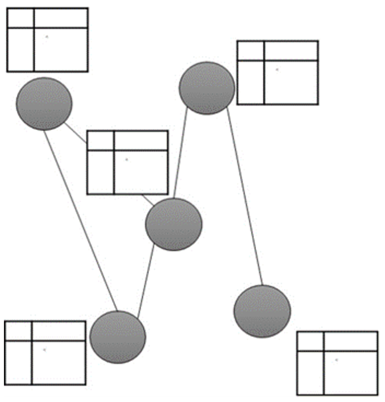
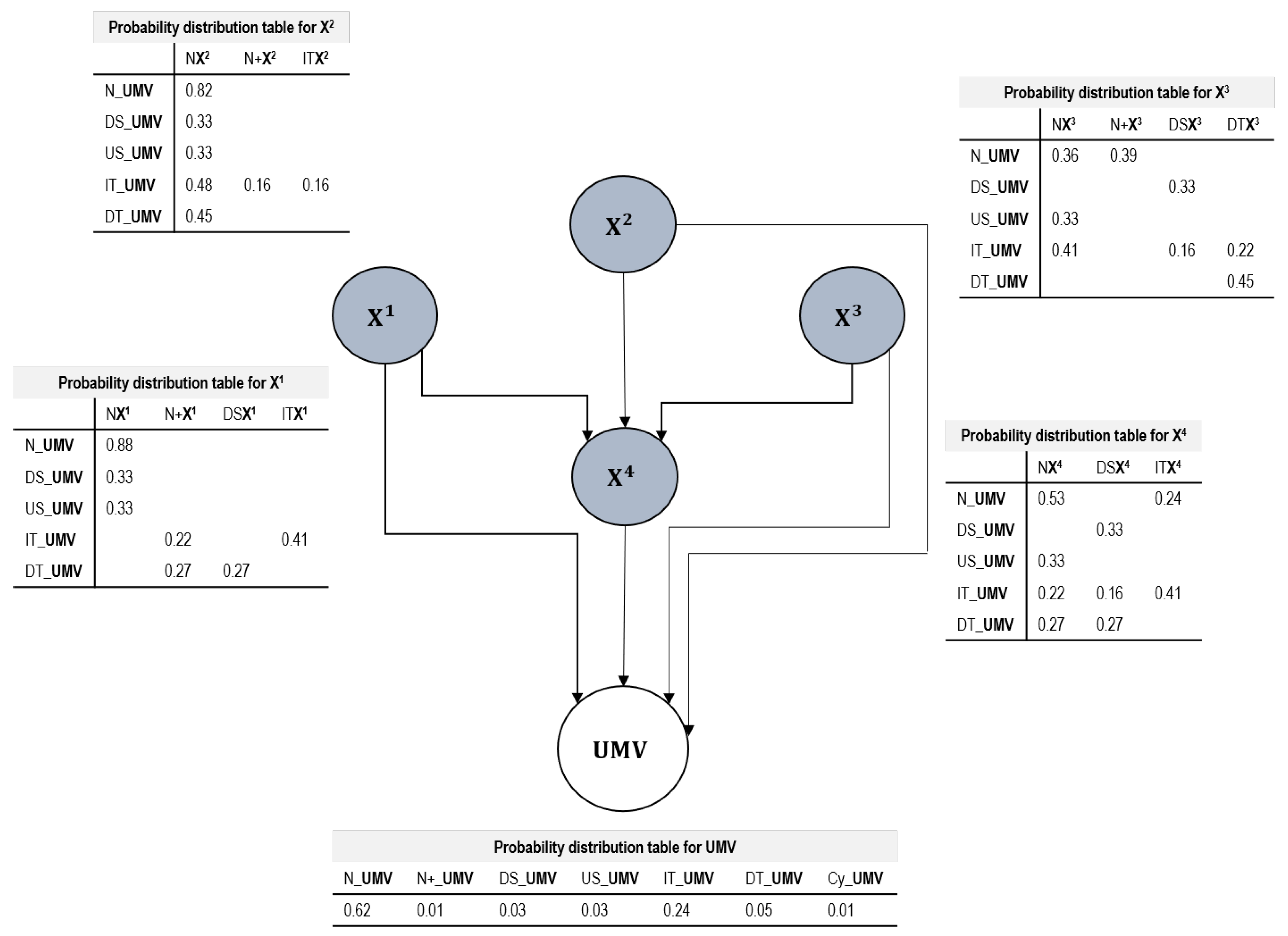
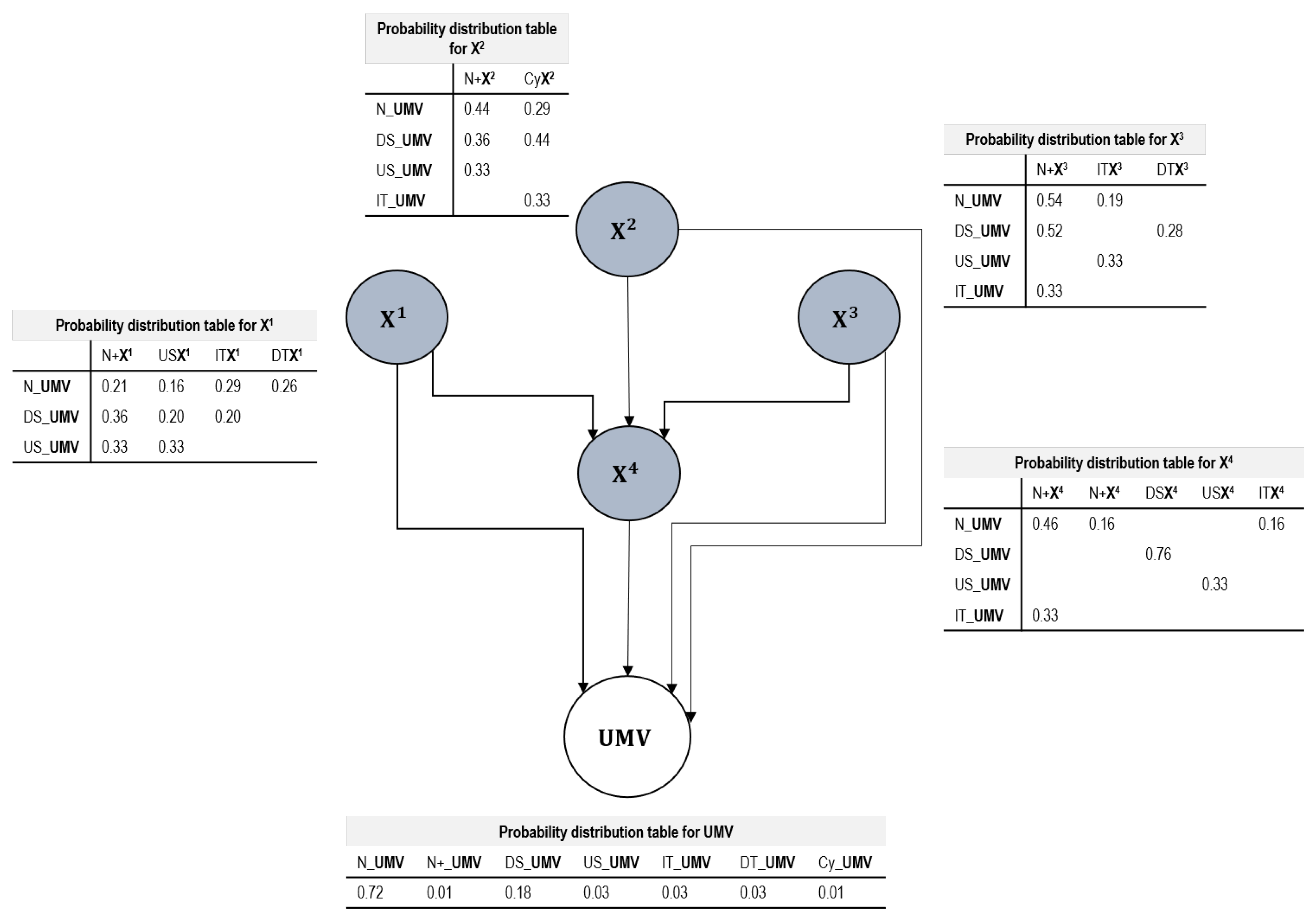
In a Bayesian Network, the data structure marks the way in which the nodes and connections are integrated, that is, the dependence and independence of each variable. A Bayesian Network is a Directed Acyclic Graph as is shown in Figure 1.

A Directed Acyclic Graph defines a factorisation of the joint probability distribution over the variables that are represented by the nodes and the factorisation is given by the directed links. For each Directed Acyclic Graph consider: (i) G = VE where V denotes a set of nodes and E, a set of directed links between pairs of nodes, (ii) a joint probability distribution $P\left(U_V\right)$ over the set of variables indexed $U_V$ by V that can be factorised as:

$$P\left(U_V\right)=\prod _{(v\in V)}P\left(U_v\right|U_{pa\left(v\right)})$$

(1)

where $U_{pa\left(v\right)}$ denotes the set of variables of the variable $U_V$ for each node $v\in V$. Factorisation expresses a set of independence assumptions that are represented by the Bayesian Network in terms of pairs of nodes that are not directly connected to each other by a directed link. The existing relationships are defined in Conditional Probability Tables attached to each node that specify the probability of a particular state given the states of the main nodes [28], which is shown in Figure 1.

The method for the Bayesian Network validation reserves a certain amount of data for testing with the rest used for confirmation. Each class in the complete data set must be represented with the correct proportions in the training and test sets. There are numerous statistical techniques for comparing models such as cross-validation, which is recommended as one of the best ways to test a model and introduces bias when testing its validity with the same data [29].

The K2 is a simple learning algorithm for Bayesian Networks. It starts with an order of nodes processing each node in turn and immediately considering adding edges of previously processed nodes to the current one. In each step, it adds an advantage that maximises the network score, and when there are no further improvements, the attention is directed to the next node. As an additional mechanism to avoid overfitting, the number of parents for each node can be restricted to a predefined maximum as stated in [30].

The problem that this article solves is located in multivariate statistics, which seeks to obtain simple methodological forms of analysis of the behaviour of several variables simultaneously. In a practical way, understanding more than two CCs to identify causes of special variation is a complex task and subject to errors, the so-called type 1 and 2 errors in classical statistics. This article shows how through the UMV it is possible to synthesise the variation of the 4 random variables of the study case. The complexity of the system is reduced from 4 to 1. Thus, the analytical inspection of the behaviour of the UMV leads to the generalisation of the 4 variables, without neglecting the fact that a special cause of variation affects more than one random variable.

A notable contribution from this research is the use of index numbers in the method. It is known that index numbers are a statistical measure allowing the study of variations of data series in relation to a measure defined as a base. The advantages are obtaining the properties of identity, proportionality, inalterability and homogeneity in the data series of the variables. Index numbers are used as a statistical measure to study variations of one or more variables with respect to time. With these, the random variables “p” that come from different measurement scales can be compared under the same scale, thus obtaining a way to compare these variations that originally have different magnitudes and units of measurement. Another contribution is the use of Bayesian Networks to calculate the probabilities that a multivariate pattern with special variation presents and the probability that it comes from the presence of some pattern of some specific univariate variable. The Bayesian Inference is an alternative approach for the identification of variables and for the MVPR without requiring the necessary assumptions made in traditional CCs methods.

The paper has been organised as follows: After this brief introduction, the study case is presented in Section 2; Section 3 formally presents our model methodology whereas simulated results and real-world case results are presented in Section 4; finally, conclusions are given in Section 5.

2. Study Case

To validate our model, simulated data and real data were used. The real data were taken from various measurements made from Gouda cheese. The cheese blocks first enter into the cutting machine where slices are cut by an automated machine. The cutting process results in small slices fit for individual packaging of predefined dimensions. There are 4 quality characteristics, weight and 3 measurements in length (thickness, width and height) as indicated in Figure 2.

The complete block of cheese has the geometric shape of a semi-regular rectangular prism with variable weight and lengths. Of the cheese slices, it is important to measure the thickness, width and height as well as record the weight of the cut slice. These are quality characteristics that consequently generate 4 random variables, X¹, X², X³ and X⁴, respectively. These univariate variables are observable for the SPC. Weight and dimensional measures have a descriptive statistical behaviour as random variables. They have trends, dispersion and, of course, parameters and estimators with accordance to the function of the probability distribution that they present. The objective is to keep the dimensions and weight in statistical control to avoid losses for the manufacturer and to improve the acceptance of the product by the customer. The statistical behaviour of the weight and dimensions of the cheese slices were studied. It is evident that there is a correlation between dimensional variables and weight.

Table 1. Summary of the statistical characteristics of the random variables of the cheese slices.

Concept	Thickness X1	Width X2	Height X3	Weight X4
Probability distribution	Non-normal	Non-normal	Non-normal	Normal, approximately with great amount of data
Variation pattern type	Variable	Variable between two or more patterns (IT and DT)	Variable	Variable
Process Observation	It is defined by the cutting machine in a self-regulating way. Overfitting is present.	It is predetermined by the variable dimension of cheese block	It is predetermined by the variable dimension of cheese block.	Correlated with the dimensions of the cheese slices.

shows a summary of the statistical analysis.

The cutting system evaluates and determines the thickness of the cheese slices with which the cutting machine adjusts the activation of the blade between slices. As this adjustment is dynamic, there is over-adjustment in the process which is explained as the action of continuous and recurrent changes of the values in the parameters of equipment, machinery or processes with the intention of causing the quality characteristics of the product to be within specs. Normally, these adjustments are carried out without the statistical bases that allow understanding of the concepts of natural and special variation.

3. Model

The developed model consists of two stages (see Figure 3). The first stage corresponds to the identification process (of variables and patterns), and the second stage refers to the process of attribution of patterns detected in the unified variable where frequencies and pattern association is achieved with the Bayesian Network.

3.1. Identification Process—Stage 1

The identification process considers:

(A)

Random Variables Definition

Consider each of the “p” univariate random variables to be analysed on Xⁱ from $i=1$ to p, where “n” is the amount of data that the random variable contains.

$$\begin{array}{c}{\mathbf{X}}^{\mathbf{1}}=\{x_1^1,x_2^1,x_3^1,\dots ,x_n^1\}\\ {\mathbf{X}}^{\mathbf{2}}=\{x_1^2,x_2^2,x_3^2,\dots ,x_n^2\}\\ ⋮\\ {\mathbf{X}}^{\mathbf{p}}=\{x_1^p,x_2^p,x_3^p,\dots ,x_n^p\}\end{array}$$

Subsequently, the matrix $\mathbf{X}$ shown in Equation (2) is constructed. According to the method of application of the CCs, considering only critical quality variables, that is, those in which the performance of the quality of the process is reflected. $\mathbf{X}$ denotes the multivariate random variable that is in turn an integrating matrix arrangement of the p univariate random variables with n observations. Thus, $\mathbf{X}$ will have dimensions of $p\times n$.

$$\mathbf{X}=\left[\begin{array}{ccc}{x}_1^1& \dots & x_n^1\\ ⋮& \ddots & ⋮\\ x_1^p& \dots & x_n^p\end{array}\right]$$

(2)

(B)

Dimensional reduction to obtain the Unified Multivariate Variable (UMV)

Obtaining the UMV is based on a reductionist approach of converting a system of variation of p univariate random variables into a single univariate random variable. The variation structures of the system of p variables are transferred to the UMV; with this, it is possible to maximise human understanding of the statistical and graphical behaviour of the system of variables. In the Statistical Control of Multivariate Processes, this reductionist principle is followed, which offers advantages in the simple analysis of the behaviour of a complex data set in a single observable data set. The obtained UMV achieves variable simplification using the random variables’ centrality and dispersion. One of the characteristics of the UMV is that it also considers each one of the observations and the statistical characteristics of all the random variables. To obtain the UMV the procedure is as follows:

(i)

Obtain the column vector of the means of X to obtain Equation (3). This vector’s dimension would be of $p\times 1$. Each row’s mean (from i = 1 to p) will be calculated for ${\overline{X}}^i=\frac{1}{n}{\sum }_{j=1}^n{x}_j^i$

$$\overline{\mathbf{X}}={[{\overline{X}}^1,{\overline{X}}^2,\cdots ,{\overline{X}}^p]}^T$$

(3)

(ii)

Generate the index numbers for each of matrix X’s elements to obtain I.

$$\mathbf{I}=\left\{\left(\begin{array}{ccc}\frac{x_1^1}{{\overline{X}}^1}& \dots & \frac{x_n^1}{{\overline{X}}^1}\\ ⋮& \ddots & ⋮\\ \frac{x_1^p}{{\overline{X}}^p}& \dots & \frac{x_n^p}{{\overline{X}}^p}\end{array}\right)\right\}=\left\{\left(\begin{array}{ccc}{I}_1^1& \dots & I_n^1\\ ⋮& \ddots & ⋮\\ I_1^p& \dots & I_n^p\end{array}\right)\right\}$$

(4)

(iii)

Generate the column vector $\mathbf{S}$ of standard sample deviations of random p variables where from $i=1$ to p of $\mathbf{X}$, $S^i=\sqrt{\frac{{\sum }_j^n{(x_j^i-{\overline{X}}^i)}^2}{n-1}}$ is applied. Equation (5) is obtained.

$$\mathbf{S}={[S^1,S^2,\dots ,S^p]}^T$$

(5)

(iv)

Obtain the vector NI with $i=1$ to p from the matrix I (indexes) using $N{I}^i={\sum }_{j=1}^n{I}_j^i=1$ to obtain:

$$\mathbf{NI}={[N{I}^1,N{I}^2,\dots ,N{I}^p]}^T$$

(6)

(v)

Compute the matrix of the index number product for the standard deviations (Equations (4) and (5)) and call this matrix $\mathbf{M}$.

$$\mathbf{M}=\left\{\left(\begin{array}{ccc}{I}_1^1{S}^1& \dots & I_n^1{S}^1\\ ⋮& \ddots & ⋮\\ I_1^p{S}^p& \dots & I_n^p{S}^p\end{array}\right)\right\}=\left\{\left(\begin{array}{ccc}{M}_1^1& \dots & M_n^1\\ ⋮& \ddots & ⋮\\ M_1^p& \dots & M_n^p\end{array}\right)\right\}$$

(7)

(vi)

Obtain the $\mathbf{N}$ vector with $i=1$ to p from $\mathbf{M}$ using $N^i={\sum }_{j=1}^n$ ${\mathrm{M}}_j^i$ to obtain:

$$\mathbf{N}={[N^1,N^2,\dots ,N^p]}^T$$

(8)

(vii)

Compute the nucleus ($N_n$) as the sum of the elements of $\mathbf{S}$ (Equation (5))

$$N_n=S^1+S^2+\dots +S^p$$

(9)

(viii)

Obtain the UMV through the product sum expressed in Equation (10)

$$\mathbf{UMV}=[(p\ast \mathbf{NI})+(N_n\ast \mathbf{N})]$$

(10)

(C)

MW construction

For each raw vector ${\mathbf{X}}^{\mathbf{i}}$ from $i=1$ to p variables and n data, a multivariate variable with predetermined length $L(L<n)$ is defined. For example, with $i=1$, the concept of multivariate variable is explained in the following manner: ${\mathbf{X}}^{\mathbf{1}}=x_1^1,x_2^1,\dots ,x_n^1$ will generate a given quantity of MW as vectors of L entries. The initial multivariate variable is formed with $x_1^1,x_2^1,\dots ,x_L^1$, and the second MW expels the data entry $x_1^1$ integrating $x_{L+1}^1$ (which is $x_2^1,x_3^1,\dots ,x_{L+1}^1$ from the initial ${\mathbf{X}}^{\mathbf{1}}$); the third vector as MW will be the initial $x_3^1,x_4^1,\dots x_{L+2}^1$

So that:

$$\begin{array}{c}\begin{array}{cc}\hfill {\mathbf{MW}}_{\mathbf{1}}& =\{x_1^1,x_2^1,\dots ,x_{L+0}^1\}\hfill \\ \hfill {\mathbf{MW}}_{\mathbf{2}}& =\{x_2^1,x_3^1,\dots ,x_{L+1}^1\}\hfill \\ \hfill {\mathbf{MW}}_{\mathbf{3}}& =\{x_3^1,x_4^1,\dots ,x_{L+2}^1\}\hfill \end{array}\\ ⋮\end{array}$$

(11)

The more data that are included in the MW, which is represented as L, the more variation characteristics in the pattern of the random variable can be recognised, and therefore the more accurate the pattern recognition will be. However, the L value cannot be too large as there is an information overload effect and this leads to confusion. In a practical approach, one could experiment with different sizes of L to determine the most suitable one. It has been found that values between 8 and 25 are adequate and also that the efficiency of pattern recognition is compromised as L increases. It is important to remember that one of the main objectives of recognition is to detect and classify patterns as quickly as possible; hence, it is important to have a convenient value for L. On the other hand, the patterns will not be displayed properly if the size of the MW is too small and consequently increases the complexity of discriminating between the different types of patterns.

To define the size of the MWs, the recommendations made in [28] are to be considered. The MWs are composed of between 4 and 24 data. As the window reduces the number of observations, the recognition quality is compromised. On the other hand, if a window with a greater number of observations is considered, better recognition precision is achieved.

(D)

Normality test for the observations of the MWs

Each MW is evaluated with an Anderson–Darling goodness-of-fit test. MWs with a p-value >0.1 are classified as having a normal probability distribution, that is, as a vector with a natural pattern; otherwise, the vector is classified as a pattern with special variation.

(E)

Diagnosis of patterns with special variation

MWs with patterns with special variation are analysed by human inspection using scatter plots to determine the pattern type and the univariate CC. In this study, the set of data of which the pattern has the characteristics of special variation with randomness not centred on the mean defined as a natural non-centred pattern (N +) is considered patterns with special variation in this study. It is assumed that the data vector looses the central reference of the mean when any of the patterns with special variation considered in this work are present.

3.2. Attribution Process—Stage 2

Stage 2 corresponds to the pattern attribution process in each MW for pattern analysis. This analysis has two objectives: (1) to account for the occurrence of each univariate variable, and (2) to distinguish the contribution of the pattern present in the UMV.

The attribution process considers:

(A)

Structural arrangement of the data

WEKA® (University of Waikato, Hamilton, New Zealand) is used for data processing, which is open source machine learning software created by the University of Waikato [31]. The software can create Bayesian Networks, Bayesian classifiers, neural networks and decision trees among other data science applications. The program requires a structural treatment of data using a file format with an extension .arff. The declared variables in this software were: Relations, Attributes and found cases (the database arrangement was defined) [25].

(B)

Configuration of the Bayesian Network

The structure of the data marks the way in which the nodes and connections are integrated, that is, the dependence and independence of each variable.

(C)

Definition of the evaluation test, estimator and of the search algorithm

Cross-validation consists of evaluation to approve the result of the Bayesian Network which allows to carry out as many evaluations as possible of data based on 10 cases. This divides the data into instances, and, in each evaluation, an instance is taken for training and another is used for evaluation. The most appropriate estimator for the network is a “simple estimator” that is responsible for finding the Conditional Probability Tables of the nodes represented in the Bayesian Network. To search for the best network configuration, a K2 scaling algorithm for the Bayesian Network is used which is restricted to find the order of the variables.

4. Results

In this section, simulated and real data will be used first to exemplify the use of the developed model, which consists of two stages. The first stage corresponds to the identification process and the second stage to the process of attribution of patterns detected in the UMV. Lastly, the model will be compared with the Hotelling’s control chart.

4.1. Analysis with Simulated Data

Data simulation to obtain X:

(A)

A matrix X is constructed with real sample data from the application case described in Section 2. In this case, $p=4$ and $n=58$, ${\mathbf{X}}^{\mathbf{1}},{\mathbf{X}}^{\mathbf{2}},{\mathbf{X}}^{\mathbf{3}},{\mathbf{X}}^{\mathbf{4}}$.

(B)

Each variable X is analysed to obtain the polynomial equation of best fit by the least squares method. The following mathematical models were obtained from the sample data at time t.

$$Y{\mathbf{X}}^1=12.9265+0.0496t-0.001547t^2+0.000013t^3$$

(12)

$$Y{\mathbf{X}}^2=2.6489+0.0591t-0.0023t^2+0.000612t^3$$

(13)

$$Y{\mathbf{X}}^3=9.9856+0.00228t-0.01301t^2+0.00018t^3$$

(14)

$$Y{\mathbf{X}}^4=398.1452+0.2537t+0.008578t^2-0.0002261t^3$$

(15)

(C)

Data are generated simulating the variation structures of the variables of X.

For our case study, it was considered that:

–

The centrality of the pattern is equivalent to the ordinate to the origin in Equations (12)–(15).

–

The temporality of the data as a time series and the mathematically modelled variation are obtained from the polynomial model.

–

Each datum point calculated using Equations (12)–(15) to obtain infinite data series was altered by adding a standard, normal and random variation component once the polynomials had been previously standardised. Equations (12)–(15) provide data vectors with fixed values since t is defined as the time scale and the polynomial defines the simulated pattern. To propose an infinite model generator of vectors based on these equations, it was necessary to include the random error term in the equations of the polynomials so that one vector is different from another in the values they contain, but similar in the pattern of the data. Therefore, the random error term produces variation in the values, but does not modify the variation structure of the data that form the pattern of the polynomial.

Thus the term $z(0,1)$ where $z\sim N(0,1)$ is added to each equation to obtain random and a large amount of data.

4.1.1. Assignment Process—Stage 1

Figure 4a shows the behaviour of one of the vectors in X. The simulated sample data were used to construct the graphs and thus visualise the patterns of the 4 univariate variables and the UMV. After analysing the variation of the data and the application of CCs, the following was found:

–

IT patterns in ${\mathbf{X}}^{\mathbf{2}}$

–

DT patterns in ${\mathbf{X}}^{\mathbf{3}}$

–

N pattern in the other two variables $({\mathbf{X}}^{\mathbf{1}},{\mathbf{X}}^{\mathbf{4}})$ with outliers.

The L value for the length of the MW was 12. With the obtained MW, 95% confidence intervals were estimated for each of the 4 variables to observe the amplitude in the variation of the data (see Figure 4b). The effect on the intervals of the DT and IT patterns as well as the outliers can be observed.

A total of 47 vectors were obtained as MW. The MWs were subjected to the Anderson–Darling non-parametric normality test to separate and identify the data from MWs with normal variation and from MWs without it. The type of variation pattern present was identified for the MWs defined with a special variation pattern as well as the UMV (see

Table 2. Patterns found in the variables and a global summary of cases found.

MW	${\mathbf{X}}^1$	${\mathbf{X}}^2$	${\mathbf{X}}^3$	${\mathbf{X}}^4$	UMV	MW	${\mathbf{X}}^1$	${\mathbf{X}}^2$	${\mathbf{X}}^3$	${\mathbf{X}}^4$	UMV	MW	${\mathbf{X}}^1$	${\mathbf{X}}^2$	${\mathbf{X}}^3$	${\mathbf{X}}^4$	UMV
1	IT	N	DS	DS	IT	17	IT	N	N	IT	IT	33	N	N	N+	N	N
2	IT	IT	DS	IT	IT	18	IT	DS	N	N	IT	34	N	N	N+	N	N
3	N	N	DS	IT	DS	19	IT	DS	N	N	IT	35	N	N	N+	N	N
4	N	N	DS	IT	N	20	US	N+	N	Cy	IT	36	N	N	N+	N	N
5	N	N	DS	IT	N	21	N+	IT	N	DS	IT	37	N	N	N+	DS	N
6	N	N	DS	DS	N	22	N+	N	N	IT	IT	38	N	N	N+	IT	N
7	N	N	N	IT	N	23	N+	N	DT	IT	IT	39	N	N	N	IT	N
8	N	N	N+	IT	N	24	N+	N	DT	DS	DT	40	N	N	N	IT	N
9	N	N	N	N	US	25	N	N	DT	IT	IT	41	N	N	N	IT	N
10	N	IT	N	N	N	26	DS	N	Cy	N	IT	42	N	N	N	DT	N
11	N	N	N	N	N	27	DS	N	DT	N	DT	43	N	N	N	N	N
12	N	N	N	N	Cy	28	DT	N	Cy	N	N	44	N	N	N+	N	N
13	N	N	N	N	N	29	N	N	US	N	N	45	N	N	N+	N	N
14	N	N	N	N	N	30	N	N	N+	N	N	46	N	DT	N+	N	N
15	N	N	N	DS	N	31	N	N	DT	N	N	47	N	N+	N+	N	N
16	IT	N	DT	IT	IT	32	N	N	N+	N	N

) in order to obtain the a priori probability by frequency counting, for Bayesian Inference.

The most frequent patterns with special variation present were: IT with 13% for X¹, N+ and IT with 6% for X², N+ with an incidence of 28% for X³ and IT of 32% for X⁴. The S and M patterns were not found in any MW. However, the pattern with special variation called N+ defined in the stage 1 point E was identified (diagnosis of pattern with special variation).

Figure 5 shows the Bayesian Network where each node represents a variable and the arcs represent the causal relationships. Each node displays its corresponding Conditional Probability Table. The Conditional Probability Table shows the probability that an event (pattern) occurs in said variable. The probabilities that are not shown in the Conditional Probability Table are due to the fact that they have an insignificant representation <0.15. The Conditional Probability Table associated with the response or resultant node shows the total probabilities of the Bayesian Inference that identifies the probability that a pattern with special variation will be present in the UMV.

4.1.2. Attribution Process—Stage 2

The structural arrangement consisted of the correct identification of variation patterns in Xⁱ and the UMV. The attributes were integrated as a .arff file for reading in WEKA® software. Figure 6 presents the structural arrangement for data entry made by up of two sections, relation and data, for the first 10 MWs. This arrangement contains three essential elements for data processing, the relation (@relation), which is the name that is assigned to the data and that allows associating the two remaining elements as part of the data set; the attributes (@attribute), which is a declaration of all possible cases of variation patterns (natural and special variation patterns) and the patterns that can occur in UMVs; finally, the description of the attributes (@DATA), which includes the declaration of the cases where each line contains the result of the analysis performed on each MW for the variables and the UMV.

The generated Bayesian Network was evaluated using Bayesian Inference with the a priori probabilities which were calculated with the data from the identification of patterns. From the UMV, the a posteriori probability was derived which is the probability that an event occurs given the experience of repeating the pattern assignments with which the network was fed many times. The evaluation of the node that operates at the UMV showed the following probabilities:

• 0.624 for a pattern N to occur,
• 0.248 for IT
• 0.05 for DT
• 0.03 for DS and for US
• 0.01 for the N + pattern
• 0.01 for C.

The N pattern in the UMV had a higher probability of occurrence because it had a higher incidence in all univariate variables. The problem of identifying multivariate patterns is to find the special variation pattern present in the variables that cause an out-of-control state in the UMV. The IT pattern showed a probability of 0.248 of presenting in the UMV. This indicates that the special variation pattern transmitted to the UMV matches with the pattern identified in Figure 7.

The Bayesian Network configuration achieved a percentage of correctly classified instances of 80.5% which means a good performance when obtaining the association of patterns.

Table 3. Conditional Probability Table related to pattern contribution.

	NX1	N+X1	DSX1	ITX1	NX2	NX3	N+X3	DTX3	DSX3	NX4	DSX4	ITX4
N_UMV	88%				82%	36%	39%			54%		25%
DS_UMV	33%				33%	33%			33%		33%
US_UMV	33%				33%	33%
IT_UMV		22%		41%	48%	41%		22%			41%
DT_UMV		27%	27%		45%			45%

shows a summary of the Conditional Probability Tables. The header shows the pattern and the variable with the highest allocation contribution. The first column describes the patterns that can occur in the UMV. The cells without information presented little or no influence.

As a result that none of the special variation patterns of the random variables presented a contribution greater than 50% of influence on the UMV, an N pattern appeared. A behaviour of IT, which was not completely defined, in the UMV was derived from the combined influence of the present patterns in the simulated variables. The variable ${\mathbf{X}}^{\mathbf{1}}$ had a 0.41 probability of causing the IT pattern in the UMV. Similarly, the N + pattern had a 22% influence on the presence of IT. In ${\mathbf{X}}^{\mathbf{3}}$, with a 22% probability of generating the special variation pattern due to a DT pattern. Finally ${\mathbf{X}}^{\mathbf{4}}$, with a 0.41 probability derived from the Cy pattern.

4.2. Analysis with Real-World Data

A set of 58 vectors were obtained for each random variable ${\mathbf{X}}^{\mathbf{i}}$ (p = 4). The 4 variables of the cheese bars are: ${\mathbf{X}}^{\mathbf{1}}$ (length in cm); ${\mathbf{X}}^{\mathbf{2}}$ (width in cm); ${\mathbf{X}}^{\mathbf{3}}$ (height in cm); and ${\mathbf{X}}^{\mathbf{4}}$ (weight in grams). The data of the four variables were segmented and grouped under the concept of MW. A significant disturbance was recognised in windows of the variable ${\mathbf{X}}^{\mathbf{4}}$ in the MW17-MW18 range. The normality of the observations was checked with the non-parametric Anderson–Darling test. For the variable ${\mathbf{X}}^{\mathbf{1}}$, the most frequent variation for the special variation pattern was IT; for ${\mathbf{X}}^{\mathbf{2}}$, the most frequent variation for the special variation pattern was Cy; for ${\mathbf{X}}^{\mathbf{3}}$, the most frequent variation for the special variation pattern was IT; and for ${\mathbf{X}}^{\mathbf{4}}$, the most frequent variation for the special variation pattern was DS. Data from vectors with non-centred natural behaviour $N+$ could be identified.

The structural arrangement was made for the identification of attributes in a file (.arff). WEKA software was used for Bayesian Network analysis. The generated Bayesian Network and its configuration were the same as that used in the simulated data cases. It was found that the pattern presented in the variables with the highest probability of occurrence was N with 0.723. The special variation pattern DS showed a probability of 0.188 of being present in the UMV which means that the pattern transmitted to the univariate variable matches with the pattern identified in the variable without treatment with the MW (see Figure 8).

The Bayesian Network configuration achieved 89.36% of correctly classified instances and that translates into a good performance when obtaining the association of patterns. A summary Conditional Probability Table is shown in

Table 4. Conditional Probability Table summary related to the pattern contribution.

	NX1	USX1	NX2	CyX2	NX3	ITX3	NX4	DSX4	USX4
N_UMV			44%		54%		47%
DS_UMV	36%		36%	44%	52%			76%
US_UMV	33%		33%			33%			33%
IT_UMV		33%		33%	33%

. Empty cells had little influence. Figure 9 shows the Bayesian Network diagram for this real data.

The probability of occurrence of a DS pattern in the univariate variable due to the presence of a DS pattern in the variable ${\mathbf{X}}^{\mathbf{4}}$ is 76%. This means that, through the Bayesian Network and in addition to predicting the type of pattern present in the UMV, the causative random variable and the type of special variation pattern are identified.

4.3. Performance of Hotelling’s Control Chart in the Study Case

To contrast the results obtained with the proposed model, the multivariate data analysis was carried out using Hotelling’s MVCC’s $T^2$. The used random variables correspond to the cheese production process. Figure 10 shows the $T^2$ CC, the set control limit and the behaviour of the multivariate variable.

Each point shown on the graph represents a sub-sample of two observations. Seven out of the control points are present, that is, they exceed the upper control limit. Although the graph shows when the process is unstable, it is not possible to identify the causative variables. The standard procedure of analysing the variables causing a control point is the use of univariate CCs. This complicates the interpretation as the number of variables to be analysed grows since the correlation between them is omitted. With the plotted points, a DT pattern was identified at the beginning of the graph and, subsequently, an IT in subgroups 13 to 24. The main limitation when identifying the patterns in the Hotelling MVCCs $T^2$ is that there are no rules for pattern interpretation. Another drawback is that the representation of the observations in the MVCCs $T^2$ is performed on a new data scale different from the one initially presented.

4.4. Considerations for the Study Case

The cheese production process has three main stages: curdling, pressing and moulding. The result of these three stages, among others involved, is reflected in the 4 quality characteristics, ${\mathbf{X}}^{\mathbf{1}},{\mathbf{X}}^{\mathbf{2}},{\mathbf{X}}^{\mathbf{3}}$ and ${\mathbf{X}}^{\mathbf{4}}$. On the other hand, the special causes of variation that produce special patterns in these 4 random variables are developed in the production method, in the machinery, equipment and tooling or in the influence of the human factor in the process. Grouping the types of special causes of variation with their effect on the 4 quality characteristics, it is concluded that the results necessarily will influence the taken action to avoid such condition in the process. A useful troubleshooting summary is useful, so that the corresponding special pattern can be dealt with as indicated in

Table 5. Summary of causes and possible solutions.

Presence of Special Pattern in	Causes	Possible Solutions
Thickness X1	(a) Machinery, equipment and tooling of the cutting machine. (b)  Influence of human factor in the operation of the cutting machine. (c) Mathematical algorithm for activation of the cutting blade that depends on the density and dimensions of the cheese block.	Cutting blade wearing. Automatic or human adjustments on the cutting machine. Modify statistical or mathematical parameters in the cutting algorithm to activate the blade. Review adjustments and their effect on cyclical, systematic patterns, trends and changes in the mean.
Width X2, Height ${\mathbf{X}}^{\mathbf{3}}$	Process stages	Check curdling and moulding by checking small or abrupt variations in X2 and ${\mathbf{X}}^{\mathbf{3}}$ of cheese block or between one block and another.
Weight X4	Depend on X1 to X3 dimensions and the cheese density	Check pressing and moulding

.

5. Conclusions

Traditional methods for pattern recognition have tried to answer three fundamental questions about what happens in the process:

1. Has a change occurred in the process?

2. When has this change occurred?

3. What are the process variables that have changed?

The first two questions are solved with the existing multivariate procedures. This novel method of MVPR using Bayesian Networks is able to answer the third question by achieving the association of patterns in a UMV. This association allowed the identification of patterns in the random variables using the concept of MW. It was observed that the graphic representation of the MWs in intervals is a smoothed and equivalent projection of the behaviour of the variables without segmentation. The Bayesian Network was able to report the types of patterns that occur in the UMV and the probability of contribution of each variable. Based on the representation of each pattern in each of the variables, the network functioned as an estimator of the patterns transmitted to the UMV.

It can be stated that it is possible to find the probabilities of occurrence of special variation pattern in the two simulated scenarios using a third degree polynomial regression. The probabilities of a pattern occurring were successfully associated using the Conditional Probability Tables provided by the Bayesian Network. In the first simulation, a correct classification of instances of 80.5% and 61.70% was found for the case of the second simulation. In both cases, the Conditional Probability Table associated the patterns found achieving the identification of the pattern present in the UMV and the influencing variable. In the case of using the network with data from a real process, the probability of occurrence of a specific pattern in the univariate variable is obtained as well as the variable that contributes the most disturbance to the identified pattern. For this scenario, a correct classification of 89.36% was achieved. This is why Bayesian Networks can be used for the association and identification of patterns that influence the UMV.

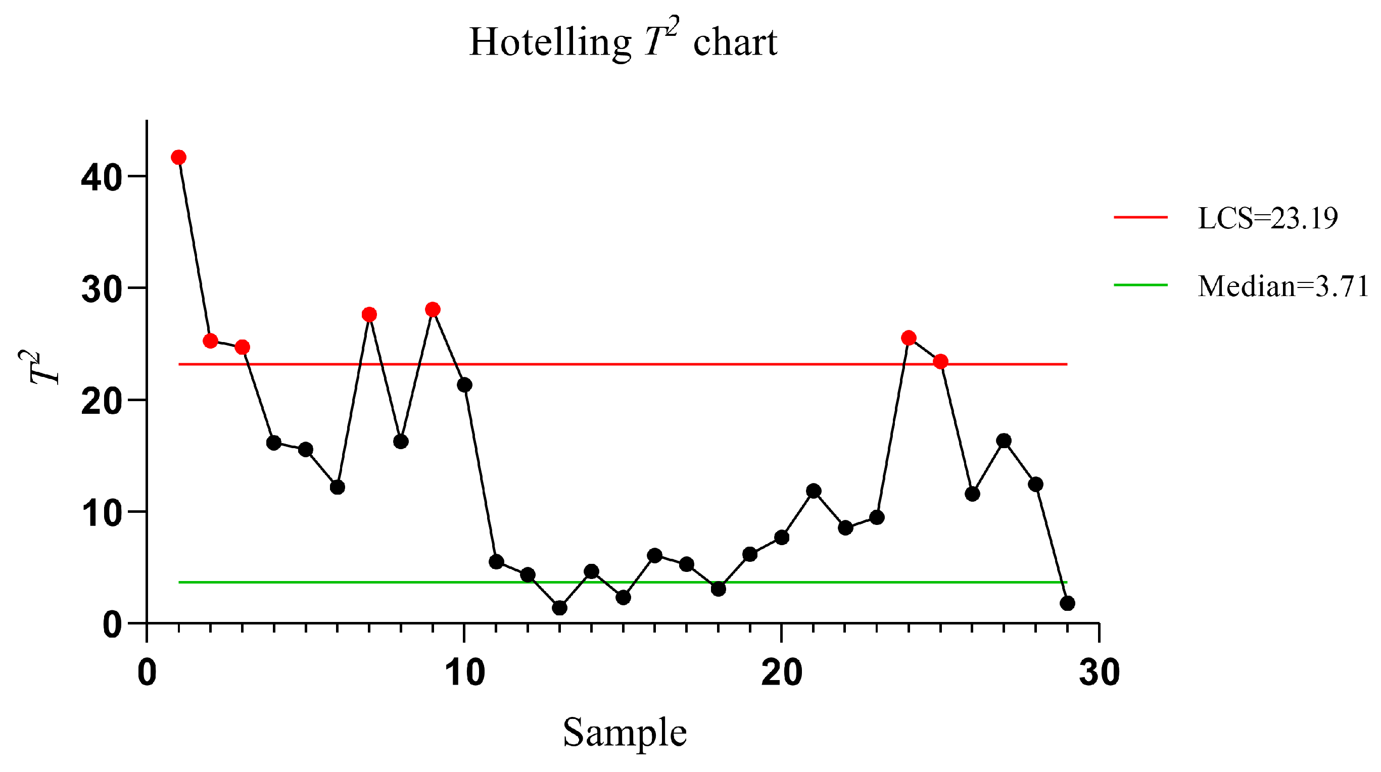
When analysing the variables of the real process with the Hotelling CC $T^2$, it was observed that the behaviour of the univariate variable does not allow inferring about the variable causing an out of control point. This problem is solved with the proposed model. For this reason, identifying the variables causing special variation pattern in multivariate processes represents our contribution with practical application in the industry. The proposed model is a new approach to pattern analysis in MVCCs using information segmentation, using multivariate variable and the analysis provided by the Bayesian Networks. This multivariate pattern recognition allows to obtain information on the random variables with the greatest influence on the UMV as well as the probability of occurrence of special variation pattern in industrial processes.

For its implementation, the following is required:

(a) A process under statistical control, using traditional statistical process control.

(b) To accomplish the programming to automate the segmentation of variables and the identification of patterns.

(c) To implement the Bayesian Network programming to generate the Conditional Probability Table and the inference about the process.

References

1. Shongwe, S.; Malela-Majika, J.C. Shewhart-type monitoring schemes with supplementary w-of-w runs-rules to monitor the mean of autocorrelated samples. Commun. Stat. Simul. Comput. 2019, 1–30. [Google Scholar] [CrossRef]
2. Krishnamoorthy, K.; Mathew, T. Statistical Tolerance Regions: Theory, Applications, and Computation; Wiley Series in Probability and Statistics; John Wiley & Sons Inc.: Hoboken, NJ, USA, 2008. [Google Scholar] [CrossRef]
3. Apley, D.W.; Lee, H.Y. Identifying Spatial Variation Patterns in Multivariate Manufacturing Processes. Technometrics 2003, 45, 220–234. [Google Scholar] [CrossRef]
4. Thomas, D. Statistical Quality Control Handbook; Western Electric Company/AT&T: Manhattan, NY, USA, 1958. [Google Scholar]
5. Hotelling, H. Multivariate Quality Control-illustrated by the air testing of sample bombsights. In Techniques of Statistical Analysis; Eisenhart, C., Hastay, M., Wallis, W., Eds.; Mc Graw Hill: New York, NY, USA, 1947; pp. 111–184. [Google Scholar]
6. Crosier, R.B. Multivariate Generalizations of Cumulative Sum Quality-Control Schemes. Technometrics 1988, 30, 291–303. [Google Scholar] [CrossRef]
7. Mason, R.L.; Champ, C.W.; Tracy, N.D.; Wierda, S.J.; Young, J.C. Assessment of Multivariate Process Control Techniques. J. Qual. Technol. 1997, 29, 140–143. [Google Scholar] [CrossRef]
8. Mason, R.L.; Chou, Y.M.; Young, J.C. Applying Hotelling’s T2 Statistic to Batch Processes. J. Qual. Technol. 2001, 33, 466–479. [Google Scholar] [CrossRef]
9. Champ, C.W.; Jones-Farmer, L.A.; Rigdon, S.E. Properties of the T2 Control Chart When Parameters Are Estimated. Technometrics 2005, 47, 437–445. [Google Scholar] [CrossRef]
10. Yeh, A.B.; Lin, D.K.J.; McGrath, R.N. Multivariate Control Charts for Monitoring Covariance Matrix: A Review. Qual. Technol. Quant. Manag. 2006, 3, 415–436. [Google Scholar] [CrossRef]
11. Chen, Y.K.; Hsieh, K.L. Hotelling’s T2 charts with variable sample size and control limit. Eur. J. Oper. Res. 2007, 182, 1251–1262. [Google Scholar] [CrossRef]
12. Reza, M.M.; Amirhossein, A.; Meysam, M.S. Step change point estimation in the multivariate-attribute process variability using artificial neural networks and maximum likelihood estimation. J. Ind. Eng. Int. 2015, 11, 505–515. [Google Scholar] [CrossRef] [Green Version]
13. Maleki, M.R. Online Monitoring and Fault Diagnosis of Multivariate-attribute Process Mean Using Neural Networks and Discriminant Analysis Technique. Int. J. Eng. 2015, 28, 1634–1643. [Google Scholar]
14. Chinas, P.; Lopez-Juarez, I.; Vazquez, J.; Osorio, R.; Lefranc, G. SVM and ANN Application to Multivariate Pattern Recognition Using Scatter Data. IEEE Lat. Am. Trans. 2015, 13, 1633–1639. [Google Scholar] [CrossRef]
15. Hernández-López, A.; Vázquez-López, J.A.; López-Juárez, I.; Lefranc, G. Pattern recognition in multivariate statistical process control for dimensional transformation of statistical parameters. In Proceedings of the 2015 CHILEAN Conference on Electrical, Electronics Engineering, Information and Communication Technologies (CHILECON), Santiago, Chile, 28–30 October 2015; pp. 19–24. [Google Scholar] [CrossRef]
16. Hernández-López, A.; Vázquez-López, J.A.; López-Juárez, I.; Baeza-Serrato, R.; Gonzalez-Calderon, R. An ensemble model for statistical monitoring of patterns in bivariate processes based on multiple artificial neuronal networks. DYNA 2020, 95, 181–186. [Google Scholar] [CrossRef]
17. Rezki, N.; Kazar, O.; Mouss, L.H.; Kahloul, L.; Rezki, D. A novel approach for multivariate process monitoring using several intelligences. Int. J. Ind. Syst. Eng. 2017, 26, 344–363. [Google Scholar]
18. Abdella, G.M.; Al-Khalifa, K.N.; Kim, S.; Jeong, M.K.; Elsayed, E.A.; Hamouda, A.M. Variable Selection-based Multivariate Cumulative Sum Control Chart. Qual. Reliab. Eng. Int. 2017, 33, 565–578. [Google Scholar] [CrossRef]
19. Marchant, C.; Leiva, V.; Cysneiros, F.J.A.; Liu, S. Robust multivariate control charts based on Birnbaum–Saunders distributions. J. Stat. Comput. Simul. 2018, 88, 182–202. [Google Scholar] [CrossRef]
20. Lin, S.Y.; Guh, R.S.; Shiue, Y.R. Effective recognition of control chart patterns in autocorrelated data using a support vector machine based approach. Comput. Ind. Eng. 2011, 61, 1123–1134. [Google Scholar] [CrossRef]
21. De la Torre-Gutiérrez, H.; Pham, D. A control chart pattern recognition system for feedback-control processes. Expert Syst. Appl. 2019, 138, 112826. [Google Scholar] [CrossRef]
22. He, F.; Mao, T.; Hu, T.; Shu, L. A new type of change-detection scheme based on the window-limited weighted likelihood ratios. Expert Syst. Appl. 2018, 94, 149–163. [Google Scholar] [CrossRef]
23. Kastner, G. Sparse Bayesian time-varying covariance estimation in many dimensions. J. Econom. 2019, 210, 98–115. [Google Scholar] [CrossRef]
24. Guh, R.S. Robustness of the neural network based control chart pattern recognition system to non-normality. Int. J. Qual. Reliab. Manag. 2005, 19, 97–112. [Google Scholar] [CrossRef]
25. Guh, R.S. Real-time pattern recognition in statistical process control: A hybrid neural network/decision tree-based approach. Proc. Inst. Mech. Eng. Part B J. Eng. Manuf. 2005, 219, 283–298. [Google Scholar] [CrossRef]
26. Song, H.; Xu, Q.; Yang, H.; Fang, J. Interpreting out-of-control signals using instance-based bayesian classifier in multivariate statistical process control. Commun. Stat. Simul. Comput. 2017, 46, 53–77. [Google Scholar] [CrossRef]
27. Ellison, A.M. An Introduction to Bayesian Inference for Ecological Research and Environmental Decision-Making. Ecol. Appl. 1996, 6, 1036–1046. [Google Scholar] [CrossRef]
28. Chen, S.H.; Pollino, C.A. Good practice in Bayesian network modelling. Environ. Model. Softw. 2012, 37, 134–145. [Google Scholar] [CrossRef]
29. Cooil, B.; Winer, R.S.; Rados, D.L. Cross-Validation for Prediction. J. Mark. Res. 1987, 24, 271–279. [Google Scholar] [CrossRef]
30. Witten, I.H.; Frank, E.; Hall, M.A. (Eds.) Data Mining: Practical Machine Learning Tools and Techniques, 3rd ed.; The Morgan Kaufmann Series in Data Management Systems; Morgan Kaufmann: Burlington, MA, USA, 2011; p. 664. [Google Scholar] [CrossRef]
31. WEKA, The Workbench for Machine Learning. Available online: https://www.cs.waikato.ac.nz/ml/weka/ (accessed on 27 December 2020).
Figure 1. General structure of a Bayesian Network.
Mathematics 09 00306 g001
Figure 2. Cheese process.
Mathematics 09 00306 g002
Figure 3. Model for Multivariate Pattern Recognition (MVPR).
Mathematics 09 00306 g003
Figure 4. X Graph considering (a) scatter plots and (b) intervals. A Unified Multivariate Variable (UMV) vector of dimension n can be seen as a representation of the values of a variable in n elements of a population, which can be seen in the graph as observations.
Mathematics 09 00306 g004
Figure 5. Bayesian Network diagram for variables from the first simulation.
Mathematics 09 00306 g005
Figure 6. Structural arrangement of the patterns found in Moving Windows (MWs).
Mathematics 09 00306 g006
Figure 7. Pattern found in the UMV.
Mathematics 09 00306 g007
Figure 8. Pattern found in UMV for real data.
Mathematics 09 00306 g008
Figure 9. Bayesian Network diagram for variables with real data.
Mathematics 09 00306 g009
Figure 10. T 2 for variables of the industrial case of cheese production.
Mathematics 09 00306 g010