
Global Portfolio Credit Risk Management: The US Banks Post-Crisis Challenge


Department of Accounting, Reporting and Financial Analysis, Wroclaw University of Economics and Business, 53-345 Wroclaw, Poland
Mathematics 2021, 9(5), 562; https://0-doi-org.brum.beds.ac.uk/10.3390/math9050562
Submission received: 12 February 2021
/
Revised: 1 March 2021
/
Accepted: 2 March 2021
/
Published: 6 March 2021
(This article belongs to the Section Financial Mathematics)
Abstract
:This paper addresses the problem of modeling credit risk for multi-product and global loan portfolios. The authors presented an improved version of the Basel Committee’s one-factor model for capital requirements calculation. They examined whether latent market factors corresponding to distinct portfolios are always highly correlated within the global portfolio and how this correlation impacts total losses distribution function. Historical losses of top-tier banks (JPMorgan Chace, Bank of America, Citigroup, Wells Fargo, US Bancorp) were analyzed. Furthermore, the estimation of the correlations between latent market factors was conducted, and its impact on the total loss distribution function was assessed. The research was performed based on consolidated financial statements for holding companies - FR Y-9C reports provided by the Federal Reserve Bank of Chicago. To verify the improved model, the authors analyzed two distinct loan portfolios for each bank, i.e., credit cards and commercial and industrial loans. They showed that the correlation between latent market factors could be significantly lower than one and disregarding this conclusion may lead to overestimating total unexpected losses. Hence, capital requirements calculated according to the IRB (Internal Ratings Based Approach) formula as a sum of individual VaR999 estimates may be biased. According to this finding, the enhanced one-factor model seems to be more accurate while calculating unexpected total loss for global portfolios. The authors proved that the active credit risk management process aiming to lower market factors’ correlation results in less volatile total losses. Therefore, financial institutions could be more resistant to macroeconomic downturns.
1. Introduction
According to the New Basel Capital Accord [1], capital requirements are expected to be calculated based on the one-factor model [2]. This methodology was implemented in more than 150 countries worldwide and allowed to calculate credit risk capital requirements using a statistical model. The purpose of this revolutionary approach was to provide more adequate loss estimates and link them with capital requirements. Furthermore, banks were encouraged to develop internal models reflecting their individual and unique risk profiles. The critical element of the recommended IRB (Internal Ratings-Based Approach) method is the probability of default (PD). The distribution function of portfolio losses depends on correlations between defaults. The correlation refers to borrowers’ assets, which determine the default event.
Under the one-factor approach, the asset correlation comes from the latent market factors. Market factor (identical for all borrowers within the examined portfolio) impacts each borrower’s asset values with the same strength. Furthermore, the asset value, and finally default event, is also determined by the idiosyncratic factor. Therefore, the loss distribution function is right-skewed. The higher the correlation, the more skewed the distribution function and the more probable the realizations of extreme losses. The rationale for it is that correlated borrowers’ assets may lead to large portfolio losses under adverse market conditions. Even though the expected value of losses stays constant, the higher sensitivity to market factors makes the loss distribution function much wider. For this reason, the critical point of the one-factor approach is a reliable estimation of asset correlation.
The economic downturn that started in 2008 revealed that banks suffered higher losses under severely adverse macroeconomic conditions than they previously expected. Therefore, the Basel Committee has encouraged banks to develop stress test models and estimate losses under adverse market scenarios. In the United States, this issue was addressed in 2011 by introducing the Comprehensive Capital Analysis and Review (CCAR) exercise. According to this exercise, the largest Bank Holding Companies (BHCs) were obliged to assess whether they can withstand potential financial stress. The Federal Reserve decided to implement new requirements towards banks with assets’ value exceeding 50 billion USD. A similar exercise was implemented in Europe by the European Banking Authority (European Union (EU)-wide stress testing). However, there are some substantial differences between US and EU approaches. First, there is a different number of adverse scenarios (three US scenarios vs. two European scenarios). Also, the methodology defined by FED (Federal Reserve) is more advanced and very precise, making it more standardized. Nevertheless, the most critical difference results from the relation between the financial regulator and the banks. FED is deemed as very demanding and strict, and therefore passing the stress test exercise is more challenging for banks in the US.
The banks are expected to calculate losses under the most plausible scenario and the severely adverse scenario.
This paper’s key challenge is to examine whether the one-factor model is accurate enough to reflect macroeconomic conditions’ volatility, especially for multi-product and multi-region loan portfolios. Currently, the one-factor approach is an industry-standard for capital requirements calculation, IFRS9 (International Financial Reporting Standard) implementation, and stress tests exercise. It is mainly due to the assets’ correlation factor inclusion, which gave model developers more flexibility in actual loss analysis. Thus, the assumptions regarding the market and idiosyncratic factors or asset correlation need thorough analysis.
There are many credit risk model applications in the literature, with particular emphasis on asset correlation. Gordy and Heitfield [3] presented the asset correlation estimation method under the multi-factor model approach. The authors leveraged Monte Carlo simulations to examine the impact of the number of observations on estimation error. S&P (Standard & Poor’s) and Moody’s data proved that the MLE (Maximum Likelihood Estimator) method gives reliable coefficient estimates. They also pointed out that a small number of defaults can significantly reduce model performance. Hamerle, Liebieg, and Rosh [4] also leveraged the MLE approach for the one-factor model. They estimated asset correlations for various business sectors and countries. They leveraged data sourced from Boegelein [5] and considered such industries as construction, agriculture, manufacturing, and services. The results revealed that the asset correlations are relatively low. Only in Japan, Germany, and Great Brittan did the correlations exceed 1%.
Low asset correlation results were also confirmed by Hamerle, Liebieg, and Sceule [6]. According to their research conducted based on corporate loans, the asset correlations appeared to be below 1%. The authors utilized more than 220 thousand observations from various industries. For correlation estimation, they used the likelihood function constructed based on individual observations (loan-level model). They also examined a wide range of macroeconomic factors that may determine credit losses.
Calem and Follain [7] verified the default values of asset correlation provided by the Basel Committee. They admitted that high values of asset correlations (e.g., 15%) might be adequate for some loan portfolios. However, Calem and LaCour-Little [8] noticed that asset correlations assigned to mortgage loans are most likely overestimated.
Also, Rosch and Scheule [9] addressed the one-factor model and credit risk estimation issue. They considered market factors as model regressors. The authors concluded that coefficient volatility might significantly impact loss projections. This finding was used for their approach, where losses under severely adverse economic scenarios were projected. The ABA data (American Bankers Association, Washington, DC, USA) were used to calculate asset correlations for several loan products, including car loans, cash loans, and credit cards. For all examined portfolios, the maximum value of asset correlation appeared to be below 3%. A similar approach was utilized by Siarka [10] for portfolio profitability analysis. He used a wide range of variables, e.g., cost of funding, remuneration costs, and expected credit loss. He showed that correlation volatility (i.e., the correlation between macro-factors) impacts portfolio profitability volatility. According to the author, it may explain loss spikes observed over time due to adverse economic conditions. Weigand [11] in his study also focused on the profitability problem. He analyzed the 20 largest banks in Japan, the US, and Europe from 2003 to 2015. He noticed that Japanese and European banks suffer due to lower net interest margins compared to US banks.
The observed discrepancies between the actual and theoretical losses volatility were examined by Lee, Lin, and Yang [12]. The authors noticed that under severely adverse macroeconomic conditions, the asset correlation might change significantly. They also pointed out that this may be a direct reason for credit losses’ uncontrolled increase under economic downturns. On the other hand, they suggested that the asset correlation can decrease during the economic boom. Owusu-Ansah [13] also referred to this problem. According to his research based on 22 US states, macro-factors were responsible for almost 28% of the PD volatility.
The US mortgage market was examined by Rossi [14]. He addressed the credit risk volatility problem of mortgage portfolios, which led to several financial institutions’ bankruptcy during the financial crisis in 2008. He concluded that many contemporary credit risk statistical models are developed based on assumptions that cannot be met. Another common problem is scarce data, which impacts model quality. He also pointed out that consideration of additional market factors may contribute to model performance improvement. Also, other portfolio breakdowns (e.g., geographical) should positively impact forecast quality.
An in-depth comparison of asset correlation estimates was presented by Siarka [15]. The author focused on retail banking, which researchers hardly explore. He presented his results (car loans portfolio) on the background of other research: Magalhaes [16], Botha [17], Crook [18], Hansen [19], Rosh [20], and Duchemin [21]. According to his research, asset correlations are not higher than 2.3%, i.e., much below the Basel Committee expectations. Kuzucu [22] showed that the real GDP (Gross Domestic Product) growth is the main determinant that affects the NPL (Non-Performing Loans) ratio. His analysis revealed that exchange rate and foreign direct investments are statistically significant for emerging countries. Vives [23] noticed that the banking sector stability depends not only on capital regulations but also on other market conditions, including competition and digital technologies.
The purpose of this paper is to examine whether the traditional approach based on the one-factor model is adequate for the global US leading banks. The authors want to examine whether a variety of business lines, such as car loans, cash loans, wholesale loans, etc., impact the overall loss distribution function. In other words, the authors want to verify the dependencies between latent market factors referring to various portfolios. For this reason, the one-factor model was enhanced by introducing another source of correlation. Finally, the two-factor models were developed for all selected banks. It is expected that this step will result in better model performance. The paper’s novelty comes from the incorporation of market factor correlation estimates to better reflect loss distribution function, giving more reliable loss forecasts.
The paper is organized as follows. The first section incorporates the introduction and the review of other researchers’ studies and defines the paper’s purpose. The next section incorporates a detailed description of the one-factor model, which the Basel Committee recommends for capital requirements calculation. Another section presents a generalized form of the model by introducing the second macro-factor. Next, the empirical results for five US banks are presented. The paper ends with a discussion, summary, and conclusions.
2. Methodology
The AIRB (Advanced Internal Rating-Based Approach) method is based on Merton’s statistical model [2]. The Basel Committee recommends it for capital requirements calculations as an efficient method of protecting banks against bankruptcy. The model allows estimating the distribution function of losses, where losses are defined as a fraction of defaulted loans in a portfolio. This approach’s idea is intuitive and based on the assumption that the default event appears when the borrower assets’ value decreases below a specific threshold limit. The value of i-th borrower assets is presented as follows:
where Y is a market factor that is identical for all borrowers over time. The rationale for it is that all borrowers are being affected by the same economic environment, and this is why they are sensitive to Y in the same way. is an idiosyncratic factor representing the borrower’s specific risk. Hence, it represents a unique borrower characteristic. Both factors directly impact the value of borrower assets . As it can be noticed, the impact of these factors on the value of the assets depends on the coefficient , which is called asset correlation. It is also assumed that both variables Z and Y are independent and normally distributed.
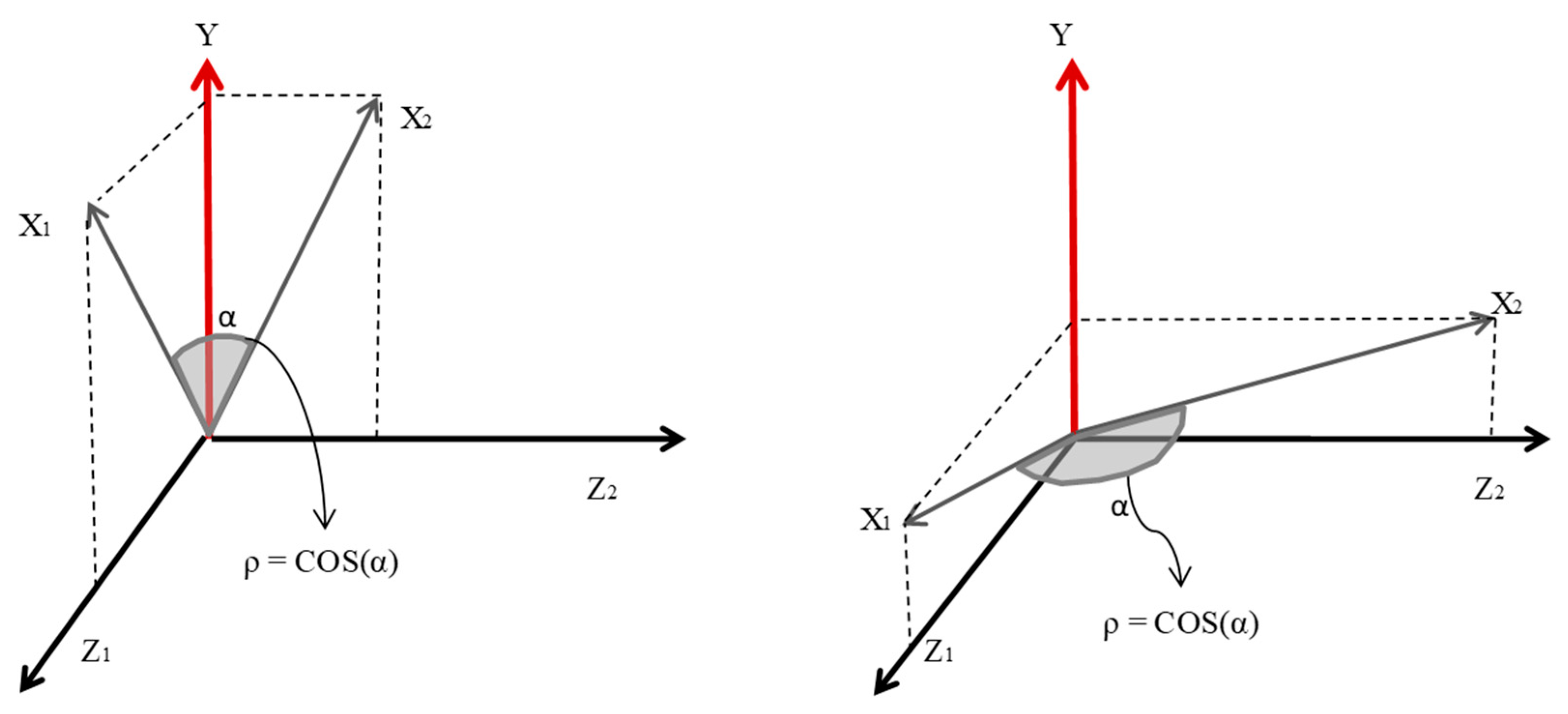
Asset correlation has an intuitive algebraic interpretation that can be visualized in three-dimensional space. For this purpose, let us assume that vector is a linear combination of vectors and Y in line with Equation (1).
Figure 1 presents a graphical interpretation of asset correlation for a portfolio consisting of two borrowers, and . is an idiosyncratic risk of the first borrower orthogonal to , i.e., and are independent, which is an underlying assumption. Market factor Y is also independent of idiosyncratic risks and . The market factor impacts asset values as the asset value is a linear combination of idiosyncratic and market factors. The asset value of the first borrower () lies in the space spanned by vectors and Y. Asset value of the second borrower is represented by vector . It can be noticed that the angle between these two vectors (borrower assets) depends on the coefficients used for a linear combination of and Y. The higher the weight assigned to market factor Y, the narrower the angle between asset values. It is a crucial finding, as the cosine of this angle is an asset correlation. The left panel of Figure 1 presents a scenario where the value of borrower assets strongly depends on the market factor. Therefore, a relatively small angle between and is observed, i.e., correlation is high. The right panel of Figure 1 shows the opposite situation, where the angle is relatively large, and the asset correlation is close to zero, as cos(90) is equal to zero.
According to the one-factor model, it is possible to calculate an asset’s threshold value that triggers a default event. When the value of assets decreases below this limit, the borrower is expected to default. The probability of default is denoted as PD. PD can also be interpreted as an expected fraction of defaulted borrowers in the portfolio. Therefore, the assets threshold limit can be calculated based on the loss distribution function. The threshold limit is straightforward to calculate based on the inverse loss distribution function. For the given expected percentage of defaulted borrowers, e.g., 3.0%, we can calculate the corresponding assets’ value as they are normally distributed. Figure 2 presents this problem in a graphical way, where the left tail of the distribution function determines the threshold limit.
As mentioned above, the default event arises when the value of assets decreases below a threshold limit α. Assuming that the variable takes one when default appears and zero in another case, we have:
As the threshold limit can be calculated as , the default always appears when:
Based on the above formula and the assumption regarding standard normal distribution of variable , the conditional (conditional on market factor Y) probability of default is:
The conditional probability of the i-th default can be interpreted as a result of a specific scenario, i.e., the market factor’s specific value. Based on a borrower’s conditional probability of default, a portfolio losses distribution function can be derived. The fraction of defaulted borrowers (portfolio loss) is defined as . It can be noticed that variables are mutually independent for the given value of variable Y [24], and they are identically distributed. Based on these findings [25], the cumulative distribution function of losses can be presented as follows:
Its density function presents the following formula:
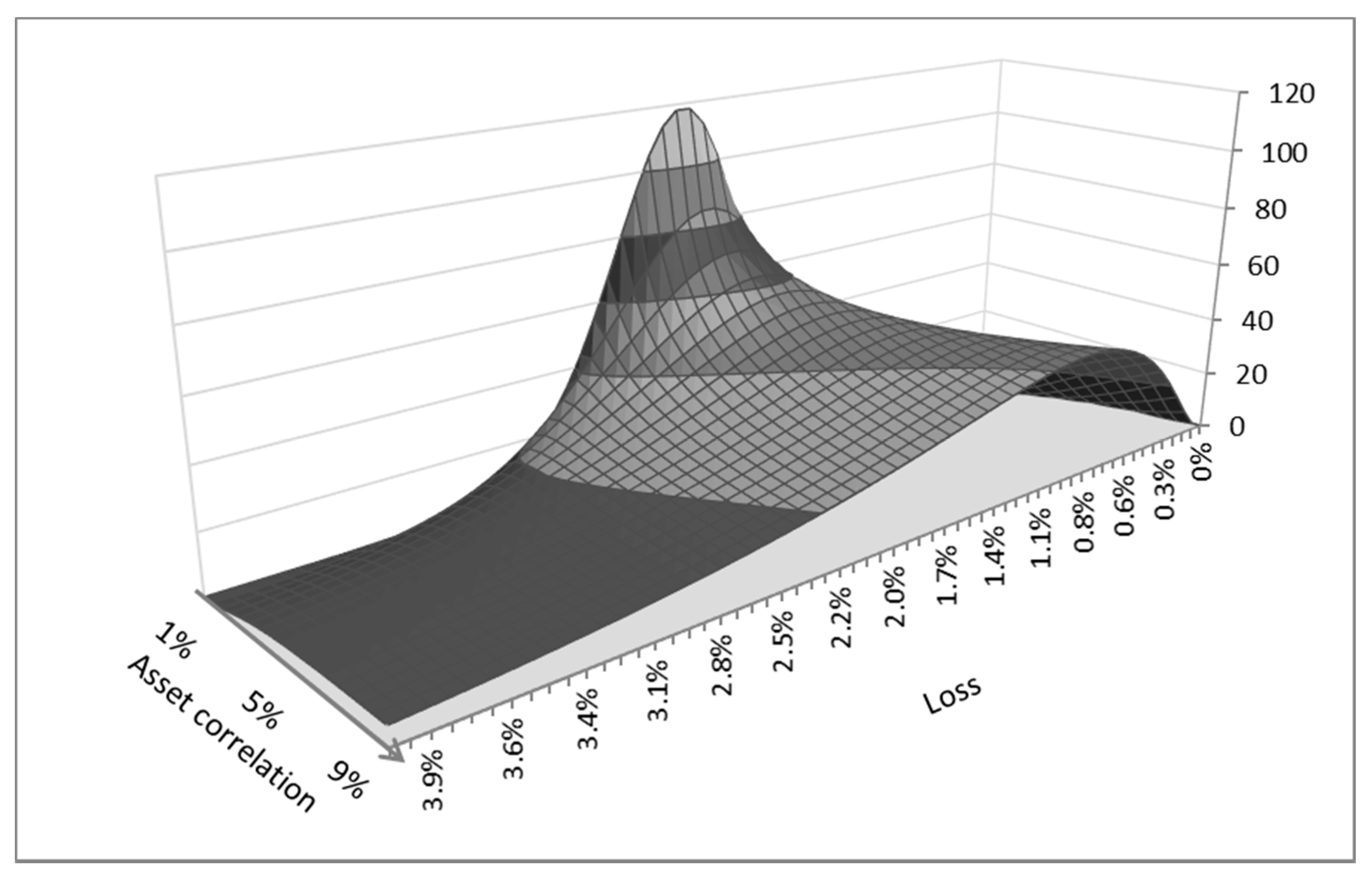
Hence, the shape of a distribution function depends on two elements, i.e., PD and . Figure 3 presents the impact of an asset correlation on the shape of the distribution function. For illustration purposes, the calculations were performed for expected loss equal to 2% and asset correlation ranging from 0% to 10%. It can be noticed that the distribution function becomes wider as the correlation grows. At the same time, the mode decreases while the expected value remains unchanged. Furthermore, the right tail of the distribution function gets fatter. Therefore, high values of losses are more likely to arise. The rationale for this is that the market factor becomes more critical once the correlation grows. Hence, we observe a reduction of the risk diversification effects resulting from independent idiosyncratic factors. Therefore, highly correlated borrowers may easily lead to enormous losses.
The assumption that there is only one significant market factor for the overall portfolio seems to be a critical model limitation. This weakness is even more apparent when considering a portfolio covering various geographical regions and/or distinct product lines. It is intuitively clear that the losses of commercial and industrial loan portfolios may be triggered by market factors that are different from the factors relating to credit card portfolios. Furthermore, a geographical breakdown may also improve loss forecasts. The borrowers located in Asia may be sensitive to different macro-factors than the US companies. Assuming that there is more than one market factor, it is essential to examine the dependencies between them. Any correlation between these market factors will impact the overall loss distribution function, i.e., total loss throughout all portfolios.
Providing that a bank has K portfolios, it can be assumed that there are K asset correlations (one for each portfolio) and also cross-portfolio correlations. Hence, the general formula presenting the specificity of an individual bank can be shown as follows:
Table 1 presents exemplary portfolio segmentation, which banks often use under CCAR (Comprehensive Capital Analysis and Review) exercise. The breakdown is based on Schedule HC-C, which is a part of the FR Y-9C report (FR Y-9C is a consolidated financial statement. This report collects basic financial data from a domestic bank holding company (BHC), a savings and loan holding company (SLHC), and a securities holding company (SHC) on a consolidated basis in the form of a balance sheet. Data are published in the Federal Reserve Bulletin and the Federal Reserve’s Uniform Bank Holding Company Performance Report (BHCPR)). These reports are submitted quarterly to appropriate Federal Reserve Banks and keep the same structures for all BHCs. Hence, it can be used for comparative analysis across the industry.
According to the presented approach, each product line has its specific asset correlation. It may result from various sensitivity of asset values to market factors and/or various composition of market factors. As was mentioned above, any market factor is latent and may vary across various portfolios. However, these market factors may be highly correlated (at least within the same geographical region). Nonetheless, the correlation between market factors must impact the overall loss distribution function.
The asset value of the i-th borrower in the k-th portfolio where F market factors were specified, can be presented as follows [26]:
where correlation matrix R (see Table 1) is a product of matrix A consisting of elements :
The conditional probability of default of the i-th borrower for given market factors can be presented by the following formula:
The above formula can be used to estimate the correlation matrix R. The number of defaults in a specific portfolio (for given values of market factors) can be modeled based on binomial distribution function as they are independent. Demey [26] proposed the following likelihood function, which leads to correlation estimates:
where is a number of observed defaults in the k-th portfolio, is a number of borrowers in the k-th portfolio, and is an unconditional probability of default in the k-th portfolio.
Under the presented approach, the number of matrix R elements requiring estimation is equal to K × (K + 1)/2. For a given segmentation (e.g., Table 1), there are 36 unknown correlations. Such a large number of coefficients requires enormous observations to get reliable estimates, and therefore it is a substantial model limitation. Therefore, a kind of simplification is highly desirable, although some information regarding cross-portfolio correlation volatility is lost. For simplicity, let us assume that various market factors are equally correlated. Based on that assumption, all elements of matrix R are the same, except diagonal elements:
Under such a simplified approach, a substantial reduction in the number of unknown elements is observed. The number of correlations is then equal to K + 1. All cross-portfolio correlations are equal; however, there are still distinct asset correlations reflecting unique risk profiles within specific portfolios.
Cespedes and Martin [27] presented an illustrative example with two latent market factors. The authors considered two separate groups of borrowers (A and B), where borrower assets were sensitive to distinct market factors, i.e., and , respectively. Furthermore, market factors were assumed to be correlated. This particular situation occurs in global portfolios where, e.g., borrowers from distinct groups (A and B) come from various geographical regions. It is expected that specific latent market factors characterize various locations. However, various economies may also interact with each other, i.e., correlations between market factors can be positive or negative. Furthermore, the underlying correlation may also result from many other possible portfolio breakdowns, e.g., product/industry/rating, etc. For instance, defaults within commercial and industrial loan portfolios are driven most likely by a market factor different from the market factor relevant to the consumer loan portfolio. In this case, these factors are expected to be positively correlated, especially under economic downturns. This particular assumption will be examined later in this paper, where five leading US banks are examined.
The following formula presents the relation between two distinct market factors:
where is N(0, 1) i.i.d. (independent and identically distributed).
Hence, the conditional probability of default (conditional on the market factor) can be presented for portfolio A and B as follow:
and
The correlation between factors must impact the overall losses distribution function, i.e., total losses observed in both portfolios. In order to illustrate that impact, a Monte Carlo simulation method was used. It was assumed that PDs were identical and equal to 3% in both portfolios for simulation purposes. Asset correlations and were also assumed to be equal (5%). Furthermore, the composition of the overall portfolio was assumed to be 50/50, i.e., the exposure values from portfolios A and B were assumed to be equal. Hence, the only factor which was changing under the simulation was correlation .
Under the simulation, two macro-factors (one for each portfolio) were randomly generated at various correlation . Moreover, 10,000 independent idiosyncratic factors were also generated for each portfolio according to Equation (1). Next, borrower asset values were calculated, and default events were identified based on assumed PD (Equation (3)). Subsequently, the underlying simulation was repeated 10,000 times at assumed market factors’ correlation. Each time, overall losses were calculated, as well as losses observed for individual portfolios. Various correlations were considered to examine its impact on the overall portfolio loss distribution function.
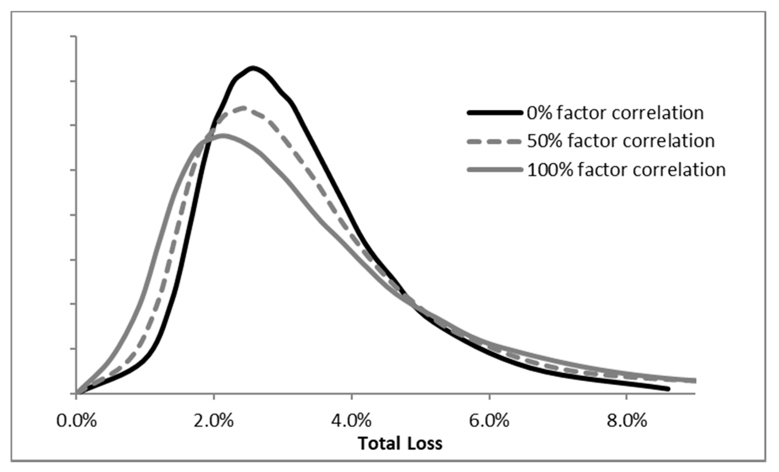
Under the Monte Carlo simulation, the following factor correlations were considered: 0%, 25%, 50%, 75%, and 100%. Figure 4 presents overall loss distribution functions derived for three selected market factor correlations (0%, 50%, 100%). It can be noticed that lower correlation makes the distribution function narrower. Hence, the unexpected loss (e.g., VaR999) gets higher when correlation rises. This finding is quite obvious, as a positive correlation weakens the portfolio diversification effect.
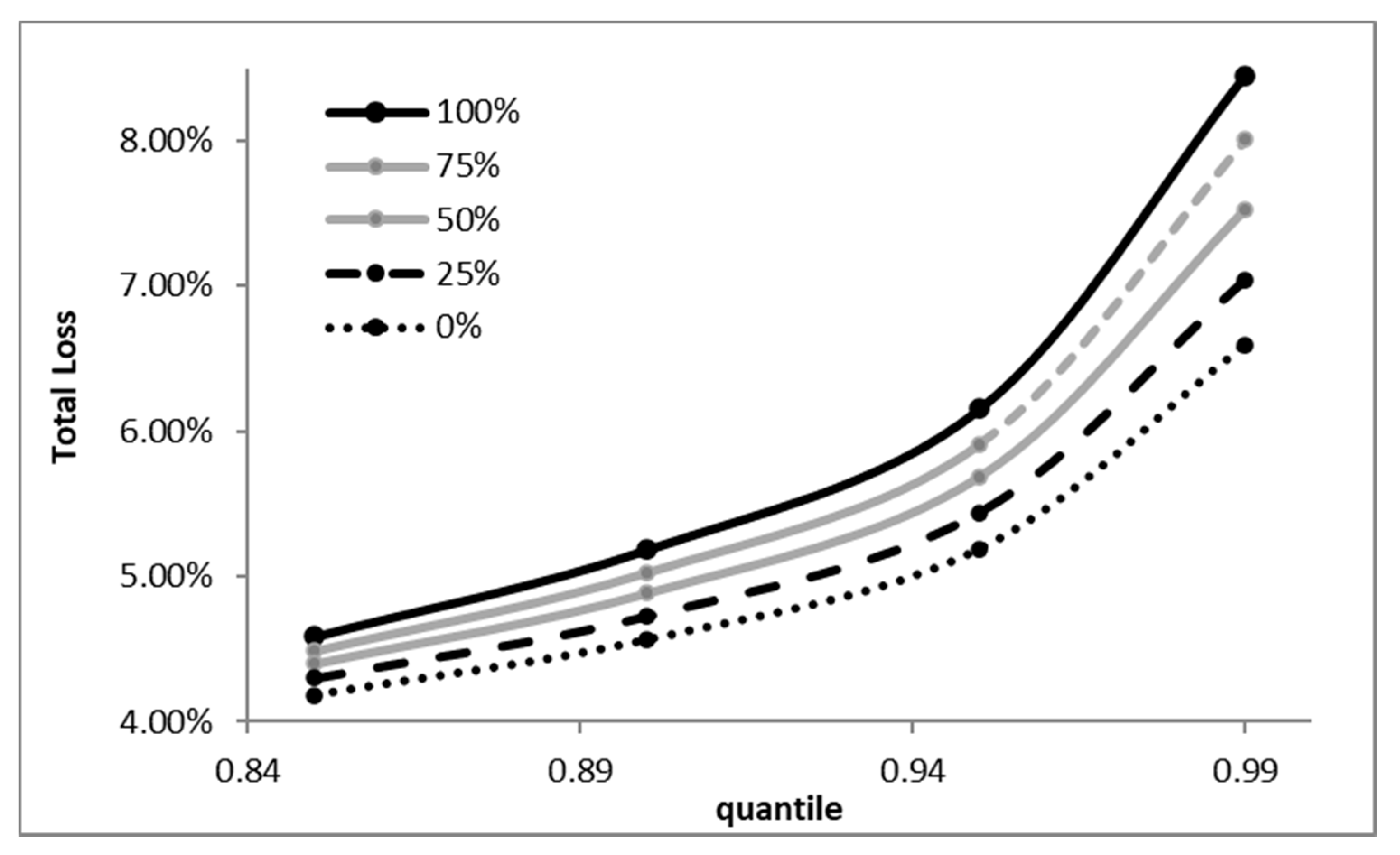
Figure 5 presents an alternative view of the simulation outcomes focusing on right tails. As underlined above, a higher correlation results in higher losses corresponding to the given quantile. Furthermore, the differences between losses are larger for higher quantiles. This finding is significant, as high quantiles correspond to severe market scenarios and are used for capital requirements calculation under the IRB approach. Therefore, market factors’ correlation is critical for capital requirements calculation and stress testing exercises.
Table 2 presents overall losses calculated under Monte Carlo simulations. The market factors’ correlation ranges from 0% to 100%, with steps of 25%. Overall losses were calculated for the following quantiles: 0.8, 0.85, 0.9, 0.95, and 0.99. It can be noticed that overall loss corresponding to quantile 0.99 rises by around 0.5% once correlation increases by 25%. Moreover, unexpected loss (VaR99) for correlation equal to 0% was estimated at 6.6%, while for correlation equal to 100%, the loss increased up to 8.4%.
The simulation results clearly show that market factor correlation may significantly impact the overall loss distribution function. This effect is especially evident for high quantiles.
3. Results
One of this paper’s critical purposes was to examine whether unexpected losses calculated for distinct portfolios are highly correlated and can be summed up to give the bank’s overall potential loss. Nowadays, bankers widely use this additive method. This approach’s rationale is that latent market factors are assumed to be equal for various portfolios even though they are not directly observed. So, under the IRB method, the correlation between latent market factors is assumed to be equal to one (i.e., perfect correlation).
This section presents the results of the analysis conducted for five leading US banks. The credit losses were calculated based on data sourced from the FR Y-9C reports (The data were downloaded from the web page: (https://www.chicagofed.org/webpages/banking/financial_institution_reports/bhc_data.cfm (accessed on 10 February 2021)). These reports are published quarterly and publicly disclosed for the United States Bank Holding Companies (BHCs). It incorporates almost two thousand database fields for each bank, including charge-offs, recoveries, outstanding values, and various product breakdowns. Currently, all BHCs with total consolidated assets above 50 billion USD are obliged to submit data every quarter. The data has been collected since 1986, and during the last 30 years, the scope has been changed multiple times, becoming more and more granular.
The FR Y-9C reports contain aggregated data, i.e., loan-level data is not available. Charge-offs and outstanding values were used for charge-off rate time series creation. The charge-off balance is the value of loans removed from the books and charged against loss reserves. Quarterly charge-off rates were calculated as a ratio of charge-offs and average portfolio outstanding for a given quarter. Hence, the charge-off rate is a risk measure similar in its nature to the default rate. However, it needs to be underlined that not every default event is automatically treated as a charge-off. Ultimately, both rates are strongly correlated and reflect the actual risk of the portfolio. For this reason, the conclusions coming from this study are valid for both risk measures.
The data regarding average quarter outstanding were sourced from Schedule HI-C—Loans and Lease Financing Receivables. The data for gross charge-offs were obtained from Schedule HI-B—Charge-Offs and Recoveries on Loans and Leases and Changes in Allowance for Loan and Lease Losses. Table 3 presents items’ codes from Schedule HI-C, and HI-B.
For the analysis, there were two types of portfolios considered, i.e., (I) credit cards and (II) commercial and industrial loans. The data were downloaded for five leading US banks, including JPMorgan Chase and Co., Bank of America Corporation, Citigroup, Wells Fargo and Company, and US Bancorp. These banks were selected due to their global span and the scale of activity measured by their assets’ value. Finally, an enhanced approach with market factors’ correlation was applied.
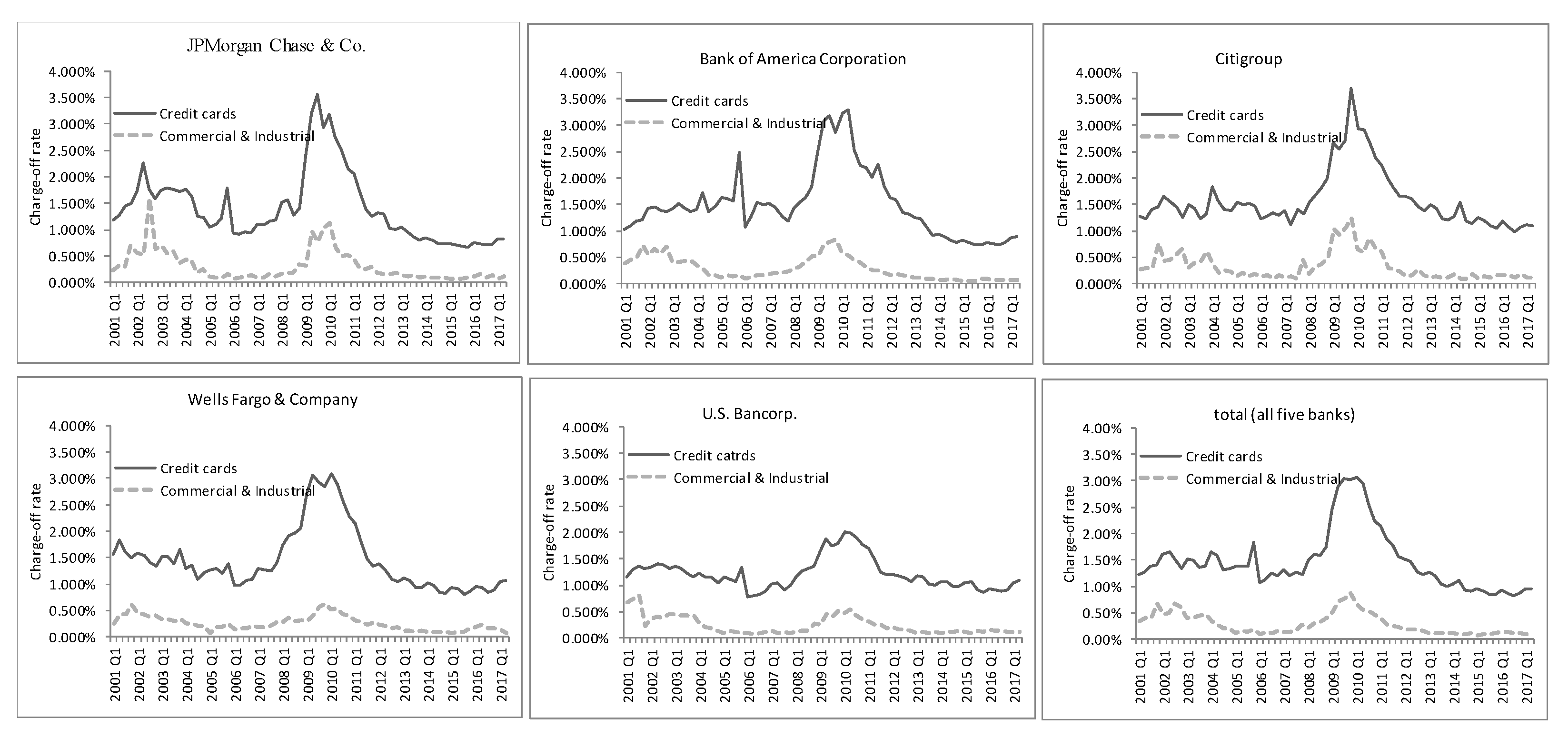
Figure 6 presents the time series of charge-off rates extracted for each bank and selected portfolios. In the sixth chart, the aggregated values for all banks are shown. It symbolizes the situation where all banks were merged (or one bank acquired other portfolios). The data used for the analysis covers the period from the first quarter in 2001 up to the second quarter in 2017, which gave 66 observations. Hence, the period of the economic downturn in 2008/2009 was included. During this turbulent period, a significant deterioration of macroeconomic factors was observed, causing significant losses to all BHCs.
The average charge-off rate for credit card portfolios across all banks was equal to 1.62%, with a standard deviation equal to 0.14%. The average rate for commercial and industrial loans was much lower, i.e., 0.33%, with a standard deviation of 0.04%. The visual analysis of Figure 6 reveals similarities between charge-off rates derived for various banks.
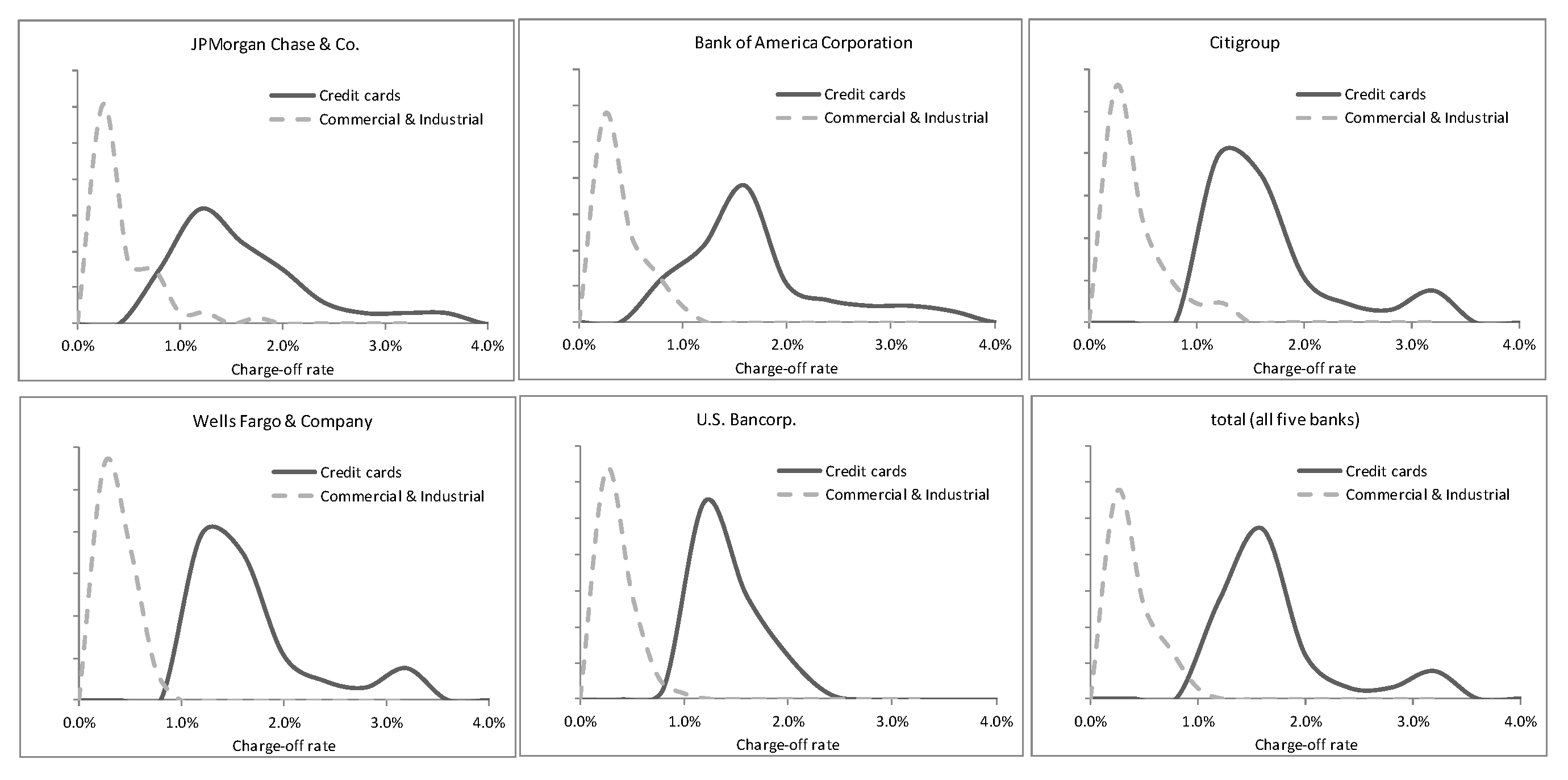
Figure 7 presents charge-off rate actual distribution functions calculated for each portfolio (credit cards and commercial and industrial loans). The results prove that the average percentage loss of commercial and industrial loans is much lower than the average loss of credit card portfolios. It can also be noticed that all actual distribution functions are right-skewed, which is in line with the one-factor approach where the right tail is ‘extended’ by the correlation. Furthermore, expected values are higher than the modes, which is also a result of positive asset correlation [15].
Next, a Monte Carlo simulation method was used for the one-factor model and the model with macro-factors correlation. Under the exercise, two portfolios for each bank were simulated. The simulation was performed at the borrower level, where idiosyncratic and market factors were randomly generated. Asset correlation was then estimated by finding the minimum value of Kolmogorov–Smirnov statistics calculated for actual and theoretical distribution functions. In other words, the best fit between theoretical and actual cumulative distribution functions indicated asset correlation.
The simulation procedure consisted of the following steps:
- The random generation of portfolios for each bank (Credit Cards, Commercial and Industrial)
- a.
- Each simulated portfolio includes 10,000 borrowers
- ▪
- Randomly generated idiosyncratic factors for each borrower,
- ▪
- Randomly generated market factor for each portfolio (CC, C&I),
- ▪
- Asset value calculations for each borrower,
- ▪
- Default events identification at the borrower level due to its specific asset value.
- b.
- The procedure (1.a) repeated 1000 times
- ▪
- Asset correlation was assumed to be identical for all borrowers within a given portfolio (one-factor model approach).
- The asset correlation estimation using Kolmogorov–Smirnov (KS) statistics (minimum KS)
- a.
- The actual charge-off rate cumulative distribution function was calculated (for each bank and each portfolio),
- b.
- Asset correlations were derived under the iterative process, where the maximum difference between actual and simulated cumulative distribution functions reached its minimum.
- Market factors’ correlations calculation
- a.
- Nominal losses (charge-off rate * actual outstanding) for each simulated portfolio were calculated,
- b.
- Based on the results (3.a.), total losses were calculated (CC + C&I) for each bank,
- c.
- Actual distribution functions of total losses for each bank were calculated,
- d.
- Market factor correlations were calculated using KS statistics for losses
- ▪
- Cumulative distribution function from points 3.b. and 3.c. were used,
- ▪
- Asset correlations from point 2 were utilized.
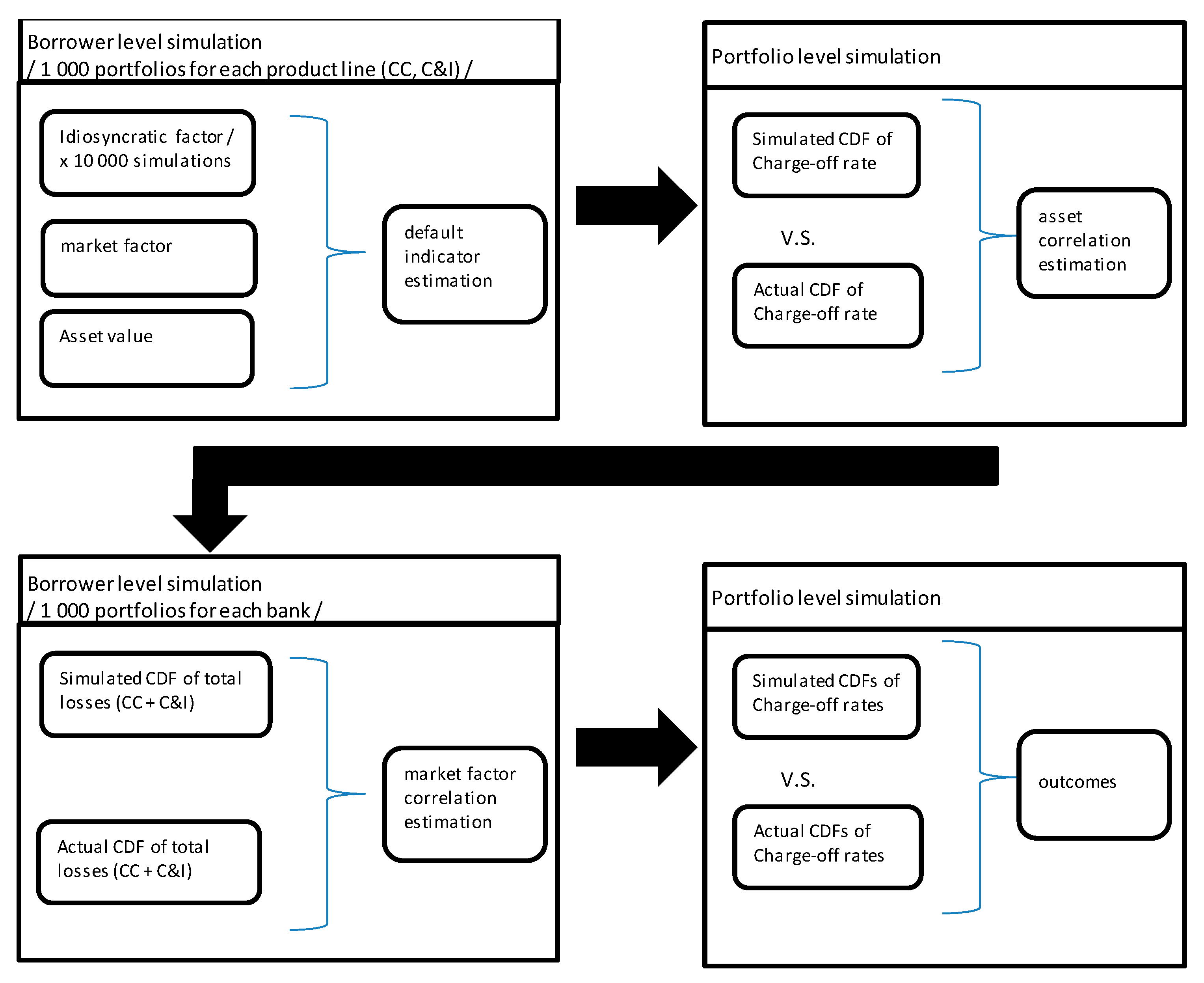
Figure 8 presents all critical steps under the simulation procedure.
The Monte Carlo simulations were performed for a given (historical) charge-off rate and a total outstanding observed at the second quarter of 2017. Charge-off rates were derived as a ratio of charge-offs and the total value of the assets. The parameters regarding portfolio expected risk and its compositions (CC/C&I) are presented in Table 4.
Table 5 presents correlation estimates derived based on Monte Carlo simulation. The first row includes asset correlations relevant to credit card portfolios (). These correlations appeared to be lower than asset correlations calculated for commercial and industrial loans (). These results are in line with Basel Committee guidances, where companies are expected to be more vulnerable to macroeconomic changes than private persons. The average asset correlation for credit cards was equal to 1.44%, with relatively small dispersion. The estimate for Bancorp was found to be relatively low (0.85%), suggesting that quarterly losses are not substantially sensitive to market conditions. For commercial and industrial loan portfolios, the impact of a market factor on borrower assets’ value appeared to be much larger as the average value was equal to 5.05%. However, estimates appeared to be quite diverse, ranging from 2.38% (Wells Fargo) to 7.31% (Bank of America).
The last row of Table 5 presents estimates of the correlation between latent market factors relevant for specified portfolios. The results are not consistent and suggest that each bank has its own product specificity. The Wells Fargo outcome shows very high correlations, reaching 98%. So, the market factors for credit cards and C&I portfolios behave nearly identically over time. When the correlation is equal to 100%, the total unexpected loss can be calculated in an additive way, i.e., as a sum of VaRs estimated independently for each portfolio. Hence, no diversification benefits are expected due to a lack of uncorrelated latent market factors.
The Bank of America, Citigroup, and JP Morgan Chase analysis shows significantly different results, where market factors appeared to be relatively low correlated. In all these cases, total losses’ distribution functions are narrower than theoretical distribution functions, where correlations were arbitrarily set to 100% (traditional IRB approach). In other words, VaR calculated for total losses (C&I and credit cards) is expected to be below the sum of VaRs calculated for each portfolio independently. A substantially lower outcome was achieved for US Bancorp, where market factors appeared to be correlated at the level of 57.52%.
The last column in Table 5 presents the outcomes for two hypothetical portfolios comprising all credit cards and C&I loans. This exercise represents a situation where all selected banks are merged. This kind of analysis is especially interesting from the market regulator’s point of view or from an investor’s perspective, where portfolio acquisitions are considered to support active risk management. It is evident that Wells Fargo may benefit from external portfolio acquisition, providing that market factors’ correlation goes down. Therefore, the best portfolio candidate for acquisition belongs to US Bancorp, where is only 57.52%. This way, the enhanced one-factor model could be leveraged. The total losses volatility could be actively reduced, making the bank more resistant to economic downturns.
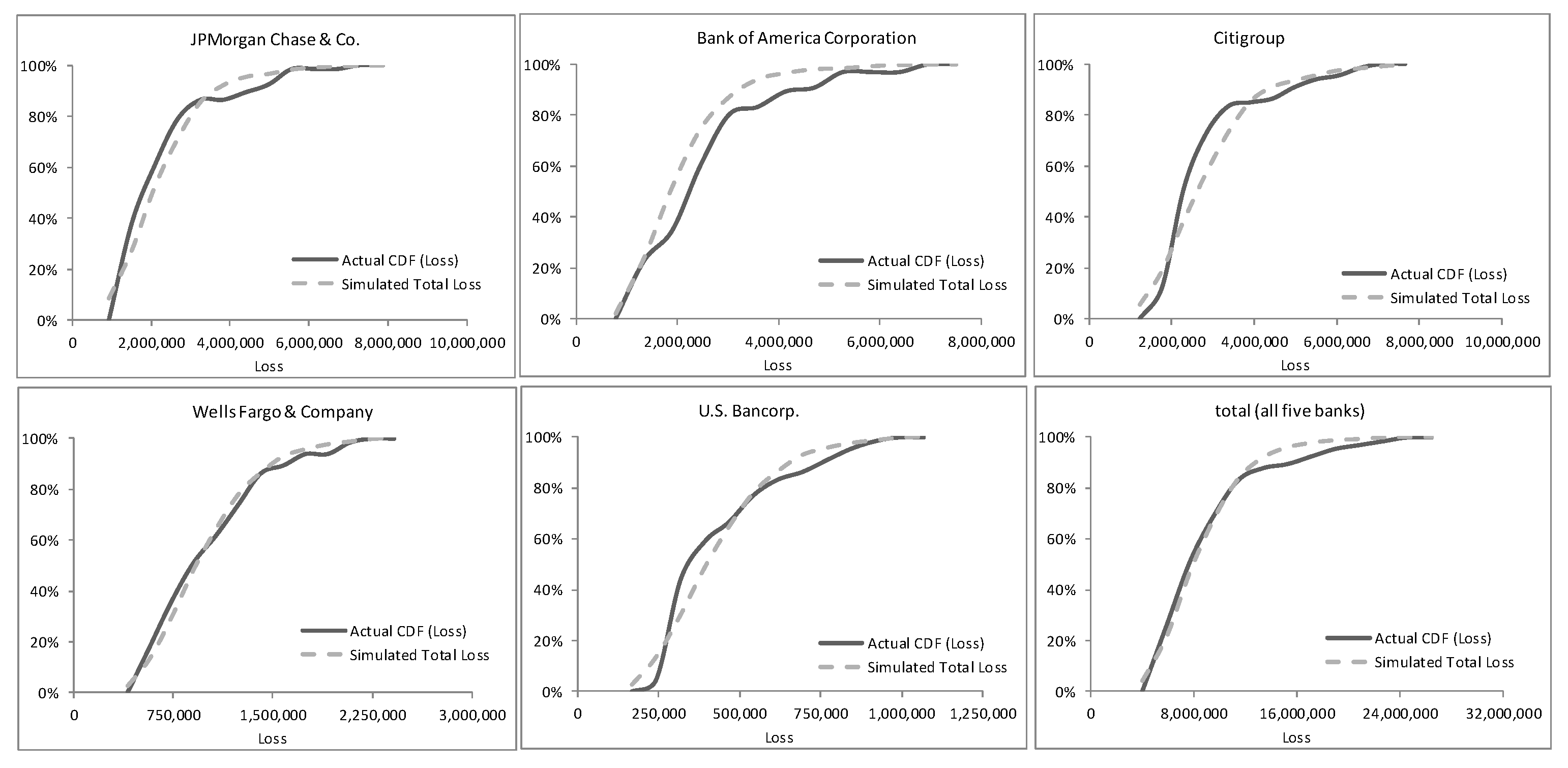
Figure 9 presents distribution functions (empirical vs. theoretical) of total nominal losses derived using the correlation between market factors. The dotted lines represent theoretical distribution functions, while the solid lines represent the actual distribution functions. The actual distribution functions were calculated based on historical charge-off rates applied for the most recent outstanding values (2017Q2). This way, nominal losses were calculated in line with the CCAR methodology. All six examples show that distribution functions (actual and simulated) are close to each other, ensuring high model performance. Later on, the results were verified with Kolmogorov–Smirnov test.
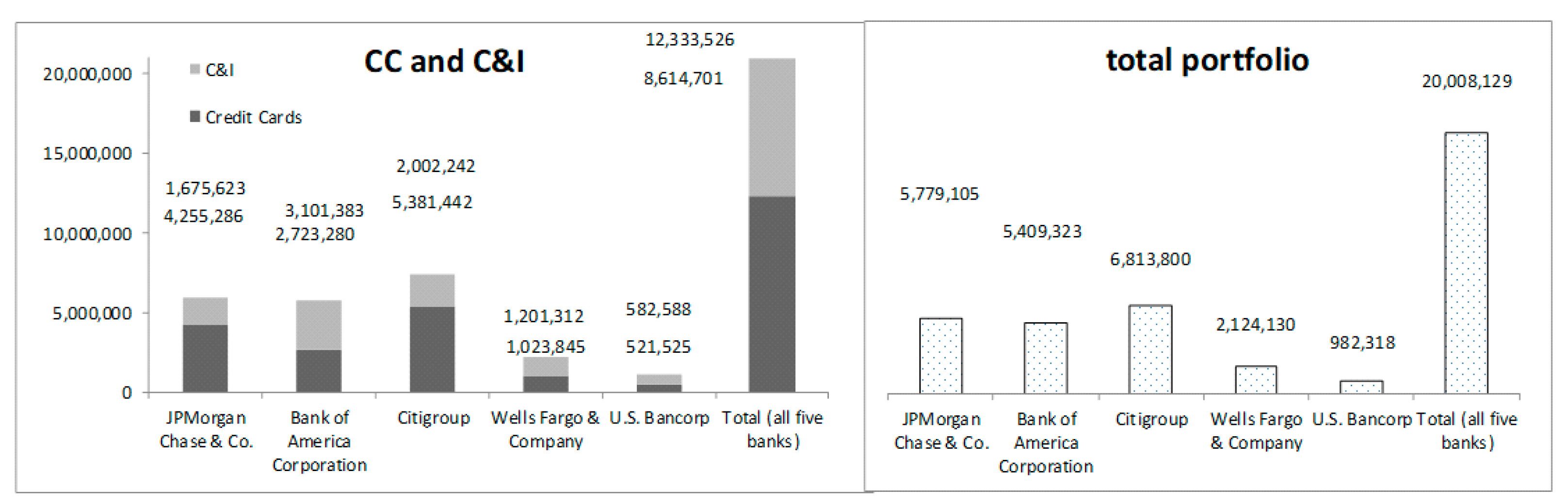
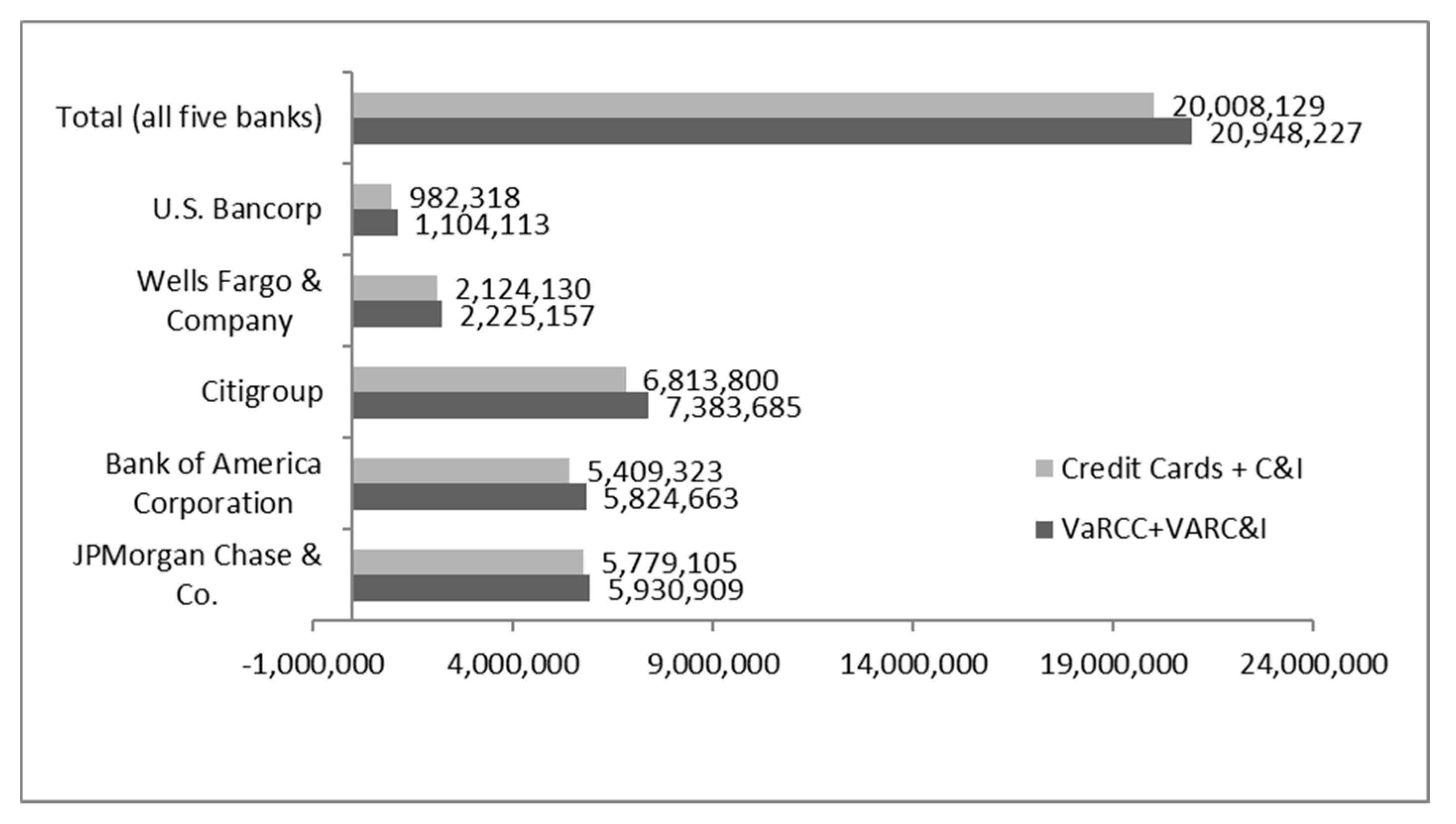
Figure 10 presents unexpected loss estimates (defined as VaR99) for various banks. The left panel shows the “additive approach” (column 5 in Table 6), assuming that the correlation is equal to one. Under this method, total unexpected loss is calculated as a sum of VaRs corresponding to specific portfolios. The right side of Figure 10 shows the results achieved for the enhanced approach, i.e., including actual market factors’ correlation. A direct comparison of the final results is presented in Figure 11.
Table 7 presents Kolmogorov–Smirnov test results for simulated and actual cumulative loss distribution functions.
As mentioned in the first part of this paper, the total unexpected loss also depends on market factors’ correlation. The lower the correlation, the larger the ‘diversification effect’ and the lower the capital requirements. However, the composition of the portfolio (credit cards outstanding vs. C&I outstanding) may efficiently disrupt expected benefits. A high imbalance may reduce the ‘diversification effect’ even though the correlation is low.
As shown in Figure 11, the bank with the highest market factors’ correlation (Wells Fargo) did not benefit due to the enhanced model. The traditional approach, where individual VaRs are summed for total losses estimation, gave nearly the same result as the enhanced one-factor model. However, Bank of America or Citigroup’s results show that the traditional approach may overestimate losses by around 8%. Furthermore, the merged banks’ results show a significant reduction of unexpected losses (21 million vs. 20 million USD).
4. Discussion and Conclusions
Adequately calculated capital requirements provide stability and safety of the financial industry. The economic downturn in 2008/2009 showed that not all financial institutions were ready to withstand severe macroeconomic conditions. For this reason, the Federal Reserve decided to implement a stress test exercise, where banks are periodically examined. According to the Board of Governors of the Federal Reserve System report [28], the losses under the severely adverse scenario are expected to be equal to 490 billion USD. Projected net revenue before provisions for loan and lease losses (PPNR) is expected to be around 310 billion USD. The aggregated tier 1 capital ratio could fall from 11.9% to 8.4%.
This paper focused on the enhanced one-factor model, showing that correlations between market factors could be calculated and used for active credit risk management. The proposed approach is adequate for total loss calculation, especially for global and multi-portfolio assets. As the FED’s data is publicly disclosed, banks and financial market regulators can easily implement the presented approach. Furthermore, the approach can be leveraged as a challenger model for bottom-up methods and constitute a benchmark solution. It needs to be underlined that latent market factors could be correlated differently in various banks/portfolios. Therefore, total loss distribution functions may vary depending on portfolio composition. Ignoring the market factors’ correlation makes sense only when it is equal to or close to one. Only then is VaRs summation methodologically justified. In other cases, the total unexpected loss may be significantly overestimated.
This research proved that the correlation between market factors relating to credit cards and commercial and industrial loan portfolios may vary across different banks. In Bank of America Corporation, JP Morgan, and Citigroup, correlations were found to be relatively low. For this reason, the total loss distribution functions are expected to be relatively narrow. The market factors’ correlations at the level close to one (e.g., Wells Fargo—98%) revealed no unexpected loss overestimation effect while using the traditional additive approach for VaRs. This research also proved that the asset correlation estimated for commercial and industrial loans is much higher than the asset correlation for credit cards. This finding is in line with other papers [15], showing (Table 5) that correlations for C&I portfolios can reach 6.0%, while credit cards oscillate around 1.5%.
The presented approach has several limitations resulting from the underlying model. Although the one-factor model seems to be quite adequate for credit risk modeling, there are still problems with the key assumptions. First, the latent macro-factor is not directly observed, and therefore its identification is a challenge. Its impact on the asset value is also difficult to interpret. While in corporate banking, ‘asset value’ has a clear theoretical interpretation, it is not easy to understand in retail banking. Definitely, in retail banking, the default causes are more complex than just a change in a borrower’s asset value. Furthermore, the one-factor model may not grasp the extreme losses observed under the economic downturns. There are still no robust theories explaining crisis causes, where macro-factors not only change, but their correlations seem to rise dramatically.
This paper’s purpose was to show that the portfolio risk management process should consider correlations between latent market factors. Higher correlation leads to higher unexpected loss due to the increase of loss volatility. This paper proved that the traditional approach to capital requirements calculation, where the portfolio’s VaRs are summed up, is quite conservative. Furthermore, the comparison of any two global banks without a deep market factors’ correlation analysis will always be biased. The bank with higher market factors’ correlation will be more risky, even though specific portfolios show equal unexpected losses.
Currently, banks are not awarded or penalized for market factors’ correlation management. So, there is no direct incentive from the capital planning point of view. This research aimed to address this issue and show that the IRB approach has some limitations for global financial institutions. As more and more financial institutions operate globally, future research needs to cover the multi-region portfolio challenge. There must be region-specific macro-factors considered for credit risk assessment. Therefore, the market practice focusing on US macro-variables needs to be improved. Furthermore, stress-test models also need revisions. The lagged variables included in the most popular in the banking industry ARMAX models (AutoRegressive Moving Average with eXogenous input) make it highly inertial. So, the models tend to respond to macro-changes with some delay, which is not the case under the economic downturn.
Funding
This research received no external funding.
Institutional Review Board Statement
Not applicable.
Informed Consent Statement
Not applicable.
Data Availability Statement
The data presented in this study are openly available in https://www.chicagofed.org/applications/bhc/bhc-home (accessed on 13 November 2020).
Conflicts of Interest
The author declares no conflict of interest.
References
- Basel Committee on Banking Supervision (BCBS). International Convergence on Capital Measurement and Capital Standards; Bank for International Settlements: Basel, Switzerland, 2006. [Google Scholar]
- Merton, R.C. On the Pricing of Corporate Debt: The Risk Structure of Interest Rates. J. Financ. 1974, 29, 449–470. [Google Scholar]
- Gordy, M.; Heitfield, E. Estimating Default Correlations from Short Panels of Credit Rating Performance Data; Working Paper; Federal Reserve Board: Washington, DC, USA, 2002.
- Hamerle, A.; Liebig, T.; Rosch, D. Benchmarking Asset Correlations. Risk 2003, 16, 77–81. [Google Scholar]
- Boegelein, L.; Hamerle, A.; Rosch, D. Econometric Approaches for Sector Analysis, forthcoming in: Lehrbass. In CreditRisk+ in the Banking Industry; Lehrbass, F., Ed.; Springer: Berlin/Heidelberg, Germany, 2003. [Google Scholar]
- Hamerle, A.; Liebig, T.; Scheule, H. Forecasting Credit Portfolio Risk, Discussion Paper Series 2: Banking and Financial Supervision. 2004. Available online: https://www.econstor.eu/handle/10419/19728 (accessed on 2 May 2019).
- Calem, P.; Follain, J. Federal Reserve Board. The Asset-Correlation Parameter in Basel II for Mortgages on Single-Family Residences. 2003. Available online: www.federalreserve.gov/generalinfo/basel2/docs2003/asset-correlation.pdf (accessed on 14 January 2018).
- Calem, P.; LaCour-Little, M. Risk-based capital requirements for mortgage loans. J. Bank. Financ. 2004, 28, 647–672. [Google Scholar] [CrossRef] [Green Version]
- Rosch, D.; Scheule, H. Stress-Testing Credit Risk Parameters: An application to retail loan portfolios. J. Risk Model Valid. 2007, 1, 55–75. [Google Scholar] [CrossRef]
- Siarka, P. Application of a loan profitability model in the process of stress testing. Bank&Credit Natl. Bank Poland 2012, 43, 81–104. [Google Scholar]
- Weigand, R.A. The performance and risk of banks in the US, Europe and Japan post-financial crisis. Investig. Manag. Financ. Innov. 2016, 13, 75–93. [Google Scholar] [CrossRef] [Green Version]
- Lee, S.C.; Lin, C.T.; Yang, C.K. The asymmetric behavior and procyclical impact of asset correlations. J. Bank. Financ. 2011, 35, 2559–2568. [Google Scholar] [CrossRef]
- Owusu-Ansah, Y. Co-Movement of State’s Mortgage Default Rates: A Dynamic Factor Analysis Approach; Working Paper; Columbia University: New York, NY, USA, 2011. [Google Scholar]
- Rossi, C.V. Anatomy of Risk Management Practices in the Mortgage Industry: Lessons for the Future; Special Report; University of Maryland: College Park, MD, USA, 2010. [Google Scholar]
- Siarka, P. Asset correlation of retail loans in the context of the new Basel Capital Accord. J. Credit Risk 2014, 10, 97–116. [Google Scholar] [CrossRef]
- Magalhaes, A.C.; Terra, J.M.M.; Neves, M.B.E. Loss Given Default: Um Estudo Sobre Perdas Emoperações Prefixadas no Mercado Brasileiro; Working Papers Series, 193; Central Bank of Brazil, Research Department: Brasilia, Brazil, 2009.
- Botha, M.; Vuuren, G. Implied asset correlation in retail loan portfolios. J. Risk Manag. Financ. Inst. 2009, 3, 156–173. [Google Scholar]
- Crook, J.; Bellotti, T. Asset Correlations for Credit Card Defaults; Working Paper; Credit Research Centre, University of Edinburgh: Edinburgh, UK, 2009. [Google Scholar]
- Hansen, M.; van Vuuren, G.; Ramadurai, K.; Verde, M. Basel II Correlation Values—An Empirical Analysis of EL, UL and the IRB Model; Credit Market Research Financial Institutions Special Report; Fitch Ratings: New York, NY, USA, 2008. [Google Scholar]
- Rosch, D.; Scheule, H. Forecasting retail portfolio credit risk. J. Risk Financ. 2004, 5, 16–32. [Google Scholar] [CrossRef] [Green Version]
- Duchemin, S.; Schmit, L.M. Asset Return Correlation: The Case of Automotive Lease Portfolios; Working Paper CEB 03/007; Solvay Business School: Brussels, Belgium, 2003. [Google Scholar]
- Kuzucu, N.; Kuzucu, S. What drives non-performing loans? Evidence from emerging and advanced economies during pre-and post-global financial crisis. Emerg. Mark. Financ. Trade 2019, 55, 1694–1708. [Google Scholar] [CrossRef]
- Vives, X. Competition and stability in modern banking: A post-crisis perspective. Int. J. Ind. Organ. 2019, 64, 55–69. [Google Scholar] [CrossRef]
- Vasicek, O. The distribution of loan portfolio value. Risk 2002, 15, 160–162. [Google Scholar]
- Vasicek, O. Limiting Loan Loss Probability Distribution; KMV Corporation: San Francisco, CA, USA, 1991. [Google Scholar]
- Demey, P.; Jouanin, J.; Roget, C.; Roncalli, T. Maximum likelihood estimate of default correlations. Risk 2004, 17, 104–108. [Google Scholar]
- Cespedes, J.C.G.; Martin, D.G. The Two-Factor Model for Credit Risk: A Comparison with the BIS II One-Factor Model. BBVA 2002. Available online: http://www.risklab.es/es/seminarios/pasados/noviembre2002-paper.pdf (accessed on 21 February 2019).
- Board of Governors of the Federal Reserve System. Dodd-Frank Act Stress Test 2015: Supervisory Stress Test Methodology and Results. 2015. Available online: http://www.federalreserve.gov/publications/default.htm (accessed on 21 March 2020).
Figure 1.
Graphical presentation of asset correlation.

Figure 2.
Threshold limit calculation for assets’ value.

Figure 3.
Loss distribution functions depending on asset correlation.

Figure 4.
Overall loss distribution functions—Monte Carlo simulation results.

Figure 5.
Total losses for various factors’ correlations.

Figure 6.
Charge-off rate time series.

Figure 7.
Charge-off rates’ density functions.

Figure 8.
Simulation procedure scheme.

Figure 9.
Distribution functions of overall losses.

Figure 10.
Total unexpected loss estimates. Left panel—one factor approach with 100% correlation. Right panel—unexpected (total) loss calculated with market factors’ correlation.
Figure 10.
Total unexpected loss estimates. Left panel—one factor approach with 100% correlation. Right panel—unexpected (total) loss calculated with market factors’ correlation.

Figure 11.
Unexpected losses comparison.


Table 1.
Asset correlation matrix—proposed segmentation.
| 1. Loans Secured by Real Estate: | 2. Loans to Depository Institutions and Acceptances of other Banks: | 3. Loans to Finance Agricultural Production and other Loans to Farmers | 4. Commercial and Industrial Loans: | 5. Loans to Individuals for Household, Family, and other Personal Expenditures | 6. Loans to Foreign Governments and Official Institutions | 7. All other Loans | 8. Lease Financing Receivables | ||
|---|---|---|---|---|---|---|---|---|---|
| 1. Loans secured by real estate: | ρ1 | … | … | … | ρ1,5 | … | … | ρ1,8 | |
| 2. Loans to depository institutions and acceptances of other banks: | ρ2 | … | … | … | … | … | … | ||
| 3. Loans to finance agricultural production and other loans to farmers | ρ3 | … | … | … | … | … | |||
| 4. Commercial and industrial loans: | ρ4 | … | … | … | ρ4,8 | ||||
| 5. Loans to individuals for household, family, and other personal expenditures | ρ5 | … | … | … | |||||
| 6. Loans to foreign governments and official institutions | ρ6 | … | … | ||||||
| 7. All other loans | ρ7 | … | |||||||
| 8. Lease financing receivables | ρ8 | ||||||||
Table 2.
Total loss results corresponding to various quantiles and factor correlation.
| Quantile | ||||||
|---|---|---|---|---|---|---|
| 0.80 | 0.85 | 0.90 | 0.95 | 0.99 | ||
| factor correlation | 100% | 4.2% | 4.6% | 5.2% | 6.2% | 8.4% |
| 75% | 4.1% | 4.5% | 5.0% | 5.9% | 8.0% | |
| 50% | 4.0% | 4.4% | 4.9% | 5.7% | 7.5% | |
| 25% | 4.0% | 4.3% | 4.7% | 5.4% | 7.0% | |
| 0% | 3.9% | 4.2% | 4.6% | 5.2% | 6.6% | |
Table 3.
The Items codes (FR Y-9C report).
| FR Y-9C Group | FR Y-9C Subgroup | HI-C—Loans and Lease Financing Receivables | HI-B—Charge-Offs and Recoveries on Loans and Leases and Changes in Allowance for Loan and Lease Losses. |
|---|---|---|---|
| 5. Loans to Indivituals for household, family, and other personal expenditures | Credit cards | BHCKB538 | BHCKB514 |
| 4. Commercial and industrial loans | To U.S. addressees | BHCK1763 | BHCK4646 |
| To non-U.S. addressees | BHCK1764 | BHCK4645 |
Table 4.
Parameter used under Monte Carlo simulation.
| Portfolio | JPMorgan Chase & Co. | Bank of America Corporation | Citigroup | Wells Fargo & Company | U.S. Bancorp. | Total (All Five Banks) | ||||||
|---|---|---|---|---|---|---|---|---|---|---|---|---|
| CoR | comp. | CoR | comp. | CoR | comp. | CoR | comp. | CoR | comp. | CoR | comp. | |
| Credit cards | 1.40% | 44.0% | 1.50% | 25.8% | 1.58% | 47.0% | 1.46% | 15.8% | 1.22% | 22.5% | 1.48% | 33.3% |
| Commercial and industrial | 0.31% | 56.0% | 0.28% | 74.2% | 0.32% | 53.0% | 0.25% | 84.2% | 0.24% | 77.5% | 0.28% | 66.7% |
Table 5.
Asset correlation estimates.
| JPMorgan Chase & Co. | Bank of America Corporation | Citigroup | Wells Fargo & Company | U.S. Bancorp. | Total (All Five Banks) | |
|---|---|---|---|---|---|---|
| 2.58% | 0.93% | 1.82% | 1.03% | 0.85% | 0.95% | |
| 4.96% | 7.31% | 5.94% | 2.38% | 4.66% | 5.45% | |
| 79.07% | 79.56% | 76.87% | 98.09% | 57.52% | 74.07% |
Table 6.
Nominal unexpected losses—simulation results.
| VaR99 | ||||
|---|---|---|---|---|
| Entity | Credit Cards | C&I | Credit Cards + C&I | VaR99 CC + VaR99 C&I |
| JPMorgan Chase & Co. | 4,255,286 | 1,675,623 | 5,779,105 | 5,930,909 |
| Bank of America Corporation | 2,723,280 | 3,101,383 | 5,409,323 | 5,824,663 |
| Citigroup | 5,381,442 | 2,002,242 | 6,813,800 | 7,383,685 |
| Wells Fargo & Company | 1,023,845 | 1,201,312 | 2,124,130 | 2,225,157 |
| U.S. Bancorp | 521,525 | 582,588 | 982,318 | 1,104,113 |
| Total (all five banks) | 12,333,526 | 8,614,701 | 20,008,129 | 20,948,227 |
Table 7.
Kolmogorov–Smirnov test results.
| Entity | p-Value |
|---|---|
| JPMorgan Chase & Co. | 0.43 |
| Bank of America Corporation | 0.08 |
| Citigroup | 0.14 |
| Wells Fargo & Company | 0.48 |
| U.S. Bancorp | 0.15 |
| Total (all five banks) | 0.44 |
Publisher’s Note: MDPI stays neutral with regard to jurisdictional claims in published maps and institutional affiliations. |
© 2021 by the author. Licensee MDPI, Basel, Switzerland. This article is an open access article distributed under the terms and conditions of the Creative Commons Attribution (CC BY) license (http://creativecommons.org/licenses/by/4.0/).
Share and Cite
MDPI and ACS Style
Siarka, P. Global Portfolio Credit Risk Management: The US Banks Post-Crisis Challenge. Mathematics 2021, 9, 562. https://0-doi-org.brum.beds.ac.uk/10.3390/math9050562
AMA Style
Siarka P. Global Portfolio Credit Risk Management: The US Banks Post-Crisis Challenge. Mathematics. 2021; 9(5):562. https://0-doi-org.brum.beds.ac.uk/10.3390/math9050562
Chicago/Turabian StyleSiarka, Pawel. 2021. "Global Portfolio Credit Risk Management: The US Banks Post-Crisis Challenge" Mathematics 9, no. 5: 562. https://0-doi-org.brum.beds.ac.uk/10.3390/math9050562
Note that from the first issue of 2016, this journal uses article numbers instead of page numbers. See further details here.