New Robust Cross-Variogram Estimators and Approximations of Their Distributions Based on Saddlepoint Techniques

Abstract

Let $\mathbf{Z}(\mathbf{s})={(Z_1(\mathbf{s}),\dots ,Z_p(\mathbf{s}))}^t$ be an isotropic second-order stationary multivariate spatial process. We measure the statistical association between the p random components of $\mathbf{Z}$ with the correlation coefficients and measure the spatial dependence with variograms. If two of the $\mathbf{Z}$ components are correlated, the spatial information provided by one of them can improve the information of the other. To capture this association, both within components of $\mathbf{Z}(\mathbf{s})$ and across $\mathbf{s}$, we use a cross-variogram. Only two robust cross-variogram estimators have been proposed in the literature, both by Lark, and their sample distributions were not obtained. In this paper, we propose new robust cross-variogram estimators, following the location estimation method instead of the scale estimation one considered by Lark, thus extending the results obtained by García-Pérez to the multivariate case. We also obtain accurate approximations for their sample distributions using saddlepoint techniques and assuming a multivariate-scale contaminated normal model. The question of the independence of the transformed variables to avoid the usual dependence of spatial observations is also considered in the paper, linking it with the acceptance of linear variograms and cross-variograms.

1. Introduction and Notation

Spatial dependence is described by a variogram in the univariate case. If there is another variable correlated with the variable of interest and we want to use its spatial information, we have to use a cross-variogram, thus extending the univariate analysis to the multivariate case.

Formally, let $\mathbf{Z}(\mathbf{s})={(Z_1(\mathbf{s}),\dots ,Z_p(\mathbf{s}))}^t$, $\mathbf{s}\in D$ be an isotropic second-order stationary multivariate spatial process, with D being a fixed subset of ${\mathbb{R}}^d$, assuming that each component $Z_i$, $i=1,\dots ,p$, has an expectation and variance constant, i.e., they do not depend on the location $\mathbf{s}$. We also assume that the covariance between two observations depends only on the distance that separates them and not on the spatial locations.

In addition, we admit that each component possesses a variogram

$$2{\gamma }_{ii}(\mathbf{h})=var(Z_i(\mathbf{s}+\mathbf{h})-Z_i(\mathbf{s})),\forall \mathbf{s},\mathbf{s}+\mathbf{h}\in D$$

where $var$ is the variance.

We measure the statistical association between the random components of $\mathbf{Z}$ with the correlation coefficients and the spatial dependence in each component with the variograms. To capture the association both within components of $\mathbf{Z}(\mathbf{s})$ and across $\mathbf{s}$, the cross-variogram is defined as ([1], p. 67, or [2], p. 229)

$$\begin{array}{ccc}\hfill 2{\gamma }_{ij}(\mathbf{h})& =& cov\left(Z_i(\mathbf{s}+\mathbf{h})-Z_i(\mathbf{s}),Z_j(\mathbf{s}+\mathbf{h})-Z_j(\mathbf{s})\right)\hfill \\ & =& E\left[(Z_i(\mathbf{s}+\mathbf{h})-Z_i(\mathbf{s}))·(Z_j(\mathbf{s}+\mathbf{h})-Z_j(\mathbf{s}))\right]\hfill \end{array}$$

$\forall \mathbf{s},\mathbf{s}+\mathbf{h}\in D$, where $cov$ means covariance and E means mathematical expectation.

This definition is for collocated data, i.e., assuming that each location (site) has all variables $Z_i$ measured, a situation that we assume all over the paper.

The results refer to the pair $(i,j)$, i.e., to a generic pair of components $Z_i,Z_j$ of the vector $\mathbf{Z}(\mathbf{s})={(Z_1(\mathbf{s}),\dots ,Z_p(\mathbf{s}))}^t$.

Let us also assume that we have a sample of $\mathbf{Z}(\mathbf{s})$ at m locations ${\mathbf{s}}_1,\dots ,{\mathbf{s}}_m$, obtaining m (p-dimensional) observations ${\mathbf{Z}(\mathbf{s}}_1),\dots ,{\mathbf{Z}(\mathbf{s}}_m)$. Hence, the data matrix is a $m\times p$ matrix where the $(l,j)$th element is the observation of component $Z_j$ at location ${\mathbf{s}}_l$.

The definition of new robust estimators against outliers of the cross-variogram and their sample distributions are the aims of this paper.

Until now, there were only two robust estimators previously defined by [3]. This author considered the covariance estimation method to obtaining two somewhat weird and difficult to apply estimators. Here, we consider the location estimation method, extending the idea considered first in [4] and followed in [5] to the multivariate case.

To do this, we start with the classical (non-robust) method-of-moments estimator, defined as

$$2\widehat{{\gamma }_{ij}}(\mathbf{h})=\frac{1}{N_h}\sum _{l=1}^{N_h}\left[(Z_i({\mathbf{s}}_l+\mathbf{h})-Z_i({\mathbf{s}}_l))·(Z_j({\mathbf{s}}_l+\mathbf{h})-Z_j({\mathbf{s}}_l))\right]$$

with the sample size being $n=N_h$ and where the cardinality of $N(\mathbf{h})=\{({\mathbf{s}}_{l_1},{\mathbf{s}}_{l_2}):{\mathbf{s}}_{l_1}-{\mathbf{s}}_{l_2}=\mathbf{h}\}$.

It is usually assumed that spatial data follow a normal distribution, but this is unrealistic because, in practice, they are contaminated by occasional outliers. For this reason, we assume in the paper a model close to the normal, i.e., a normal-like model in the central region but with heavier tails than the normal, namely, a multivariate-scale-contaminated normal distribution with joint probability density function (pdf):

$$f_M(\mathbf{z})=f_M(z_1,\dots ,z_p)=(1-ϵ)f_N(\mathbf{z};\mathbf{\mu },\mathbf{\Sigma })+ϵf_N(\mathbf{z};\mathbf{\mu },g^2\mathbf{\Sigma })$$

(1)

where $ϵ\in (0,1)$; $g>1$; $f_N(\mathbf{z};\mathbf{\mu },\mathbf{\Sigma })$ denotes the pdf of a p-variate normal random vector with mean vector $\mathbf{\mu }=({\mu }_1,\dots ,{\mu }_p)$ and covariance matrix $\mathbf{\Sigma }$, a matrix with values ${\sigma }_i^2$ in its diagonal, $i=1,\dots ,p$.

In this framework, $ϵ$ represents the small proportion of outliers in the sample (e.g., the proportion of extreme weather events affecting $\mathbf{Z}$ at all locations) and g represents the extent of the contamination. If $ϵ=0$ or $g=1$, this model reduces to the multivariate normal distribution and, if $ϵ>0$ and $g>1$, it resembles the normal in the central part but with heavier tails.

This is the usual way in which robust statistics handles the nonnormality of the data: establishing a neighborhood of the standard model distribution, the contamination neighborhood, inside which the underlying model is located (e.g., [6,7,8], p. 12, or [9], p. 870).

From this joint distribution, the marginal distributions of the $Z_i$ are the univariate scale contaminated normal models:

$$(1-ϵ)N({\mu }_i,{\sigma }_i^2)+ϵN({\mu }_i,g^2{\sigma }_i^2).$$

The paper is organized as follows. In Section 2, we consider a consecutive pair of transformations of the initial observations to avoid their dependence. With these, we can use standard techniques for independent and identically distributed (iid) random variables. We also obtain in that section the distribution of these new variables. Here, we have a remarkable difference with respect to the paper by [5]: there, the transformed variables were the square of standard normal variables, i.e., ${\chi }^2$ distributed random variables, but here, we have the product of two different normal variables.

In Section 3, cross-variogram M-estimators based on the new variables are defined. The von Mises plus saddlepoint (VOM+SAD) approximations for their distributions are also obtained, approximations that are applied to the classical method-of-moment estimator in Section 4. This is the first time that a closed form approximation of its distribution is obtained. Simulations of approximation accuracy and lack of robustness of its distribution are included.

In Section 5, we define the $\alpha$-trimmed cross-variogram estimator and we obtain the VOM+SAD approximation for its distribution. We do the same for the Huber’s cross-variogram estimator in Section 6. We include here a simulation study to compare the robustness of the three estimators as we increase the degree of contamination.

Section 7 is devoted to analyzing the dependence of the transformed variables on the linearized cross-variogram models. We conclude the paper with two examples of real data.

Finally, in Section 8, we give some conclusions, ending the paper with an Appendix, which contains the technical details obtained in the paper.

2. Preliminary Transformation

The usual dependence between spatial observations $\mathbf{Z}$ does not allow for the use of techniques for iid variables. Nevertheless, it is possible to skip this restriction by transforming the initial observations $\mathbf{Z}$.

Namely, let us define the gap or lag variable $W_s^i$ as

$$W_s^i=W_{\mathbf{s}}^i(\mathbf{h})=Z_i(\mathbf{s}+\mathbf{h})-Z_i(\mathbf{s}).$$

The cross-variogram is now

$$2{\gamma }_{ij}(\mathbf{h})=E\left[W_s^i·W_s^j\right]$$

the mean of the product, and its classical estimator, the method-of-moments estimator,

$$2\widehat{{\gamma }_{ij}}(\mathbf{h})=\frac{1}{N_h}\sum _{l=1}^{N_h}{W}_{s_l}^i·W_{s_l}^j$$

The sample mean of the variables $X_l=W_{s_l}^i·W_{s_l}^j$, $l=1,\dots ,n$, is non-robust then.

This is the reason why we say that we use the location estimation way: the parameter is the mean, and the classical estimator is the sample mean. In this manner, instead of considering a weird estimator for a strange parameter of the initial distribution, we propose to transform the original (and usually dependent) observations $Z_l$ into new data $X_l$ (independent under some conditions) obtaining a natural parameter of the new variable (its mean) for which a manageable estimator (the sample mean) should be feasible. Then, standard techniques of robustification can be applied.

This idea has been successfully applied, first, in [4] and in [5].

An important problem is determining the distribution of this new variable $X_l$ from the original normal (or contaminated normal) distribution of $Z_l$ to later obtain the distribution of the robust estimators obtained, where $X_l$ is now the product of two different normal variables.

2.1. Correlation between $W_t^i$ and $W_s^j$

First, let us define two new functions that are natural extensions of the similar ones associated with the variogram.

Let us call cross-covariogram between $Z_i$ and $Z_j$ to the function (provided it is well defined)

$$C{C}^{ij}(|\mathbf{a}-\mathbf{b}|)=cov(Z_i(\mathbf{a}),Z_j(\mathbf{b}))$$

that will be equal to $E[Z_i(\mathbf{a})·Z_j(\mathbf{b})]-{\mu }_i·{\mu }_j$.

Here, a will be t or t + h and b will be s or s + h, and thus, ${\mu }_i=E\left[Z_i(\mathbf{t}+\mathbf{h})\right]=E\left[Z_i(\mathbf{t})\right]$ and ${\mu }_j=E\left[Z_j(\mathbf{s}+\mathbf{h})\right]=E\left[Z_j(\mathbf{s})\right]$, where the equality between the expectations is obtained because of the intrinsic stationary property of the components of Z.

Analogously, we assume the equality of the variances in locations that are distanced by a lag h, ${\sigma }_i^2=V\left[Z_i(\mathbf{t}+\mathbf{h})\right]=V\left[Z_i(\mathbf{t})\right]$, and ${\sigma }_j^2=V\left[Z_j(\mathbf{s}+\mathbf{h})\right]=V\left[Z_j(\mathbf{s})\right]$.

Let us also define the cross-correlogram as

$${\rho }^{ij}(|\mathbf{h}|)=\frac{C{C}^{ij}(|\mathbf{h}|)}{{\sigma }_i·{\sigma }_j}$$

Now, the covariance between $W_t^i$ and $W_s^j$ will be (see the Appendix A for details)

$$cov\left(W_t^i,W_s^j\right)={\sigma }_i{\sigma }_j\left[2{\rho }^{ij}(|\mathbf{t}-\mathbf{s}|)-{\rho }^{ij}(|\mathbf{t}-\mathbf{s}+\mathbf{h}|)-{\rho }^{ij}(|\mathbf{t}-\mathbf{s}-\mathbf{h}|)\right].$$

Thus, the correlation between $W_t^i$ and $W_s^j$ will be zero if

$$2{\rho }^{ij}(|\mathbf{t}-\mathbf{s}|)-{\rho }^{ij}(|\mathbf{t}-\mathbf{s}+\mathbf{h}|)-{\rho }^{ij}(|\mathbf{t}-\mathbf{s}-\mathbf{h}|)=0.$$

Because locations are fixed in advance (for instance, they could be sample stations) we assume that they are equally spaced on a transect, for instance, in Figure 2.1 of [1], i.e., they are data on a regular grid. Hence, we can match two contiguous $Z_i$ (for which the dependence is supposed to be the strongest), so that it is t + h = s.

Now, the previous condition of correlation equal to zero is obtained if

$$2{\rho }^{ij}(\mathbf{h})-{\rho }^{ij}(\mathbf{0})-{\rho }^{ij}(2\mathbf{h})=0$$

or, in terms of the cross-covariogram, when

$$2C{C}^{ij}(\mathbf{h})-C{C}^{ij}(\mathbf{0})-C{C}^{ij}(2\mathbf{h})=0.$$

(2)

On the other hand, with a little of algebra, the cross-variogram can be expressed as (see Appendix A for details)

$$2{\gamma }_{ij}(\mathbf{h})=2\left[C{C}^{ij}(\mathbf{0})-C{C}^{ij}(\mathbf{h})\right]$$

i.e.,

$$C{C}^{ij}(\mathbf{h})=C{C}^{ij}(\mathbf{0})-{\gamma }_{ij}(\mathbf{h})$$

and then, it will be

$$C{C}^{ij}(2\mathbf{h})=C{C}^{ij}(\mathbf{0})-{\gamma }_{ij}(2\mathbf{h}).$$

Replacing these values of $C{C}^{ij}(\mathbf{h})$ and $C{C}^{ij}(2\mathbf{h})$ in (2), we obtain

$$2\left[C{C}^{ij}(\mathbf{0})-{\gamma }_{ij}(\mathbf{h})\right]-C{C}^{ij}(\mathbf{0})-\left[C{C}^{ij}(\mathbf{0})-{\gamma }_{ij}(2\mathbf{h})\right]=0$$

i.e., the correlation between $W_t^i$ and $W_s^j$ will be 0 when

$${\gamma }_{ij}(2\mathbf{h})=2{\gamma }_{ij}(\mathbf{h})$$

i.e., if a linear cross-variogram can be accepted as model (because, theoretically, the nugget is 0).

Remark 1.

The increments $W_t^i$ and $W_s^j$ have as joint cumulative distribution function, if they are uncorrelated,

$$\begin{array}{ccc}\hfill P_{(1-ϵ)f_{{\mathbf{N}}_{\mathbf{1}}}+ϵf_{{\mathbf{N}}_{\mathbf{2}}}}\left\{W_t^i\le x,W_s^j\le y\right\}& =& (1-ϵ)P_{f_{{\mathbf{N}}_{\mathbf{1}}}}\left\{W_t^i\le x,W_s^j\le y\right\}\hfill \\ & & +ϵP_{f_{{\mathbf{N}}_{\mathbf{2}}}}\left\{W_t^i\le x,W_s^j\le y\right\}\hfill \\ & =& (1-ϵ)P_{f_{{\mathbf{N}}_{\mathbf{1}}}}\left\{W_t^i\le x\right\}{P}_{f_{{\mathbf{N}}_{\mathbf{1}}}}\left\{W_s^j\le y\right\}\hfill \\ & & +ϵP_{f_{{\mathbf{N}}_{\mathbf{2}}}}\left\{W_t^i\le x\right\}{P}_{f_{{\mathbf{N}}_{\mathbf{2}}}}\left\{W_s^j\le y\right\}\hfill \end{array}$$

Hence, if $W_t^i$ and $W_s^j$ are uncorrelated, with probability $1-ϵ$, they are independent under model $f_{{\mathbf{N}}_{\mathbf{1}}}$ and, with probability $ϵ$, they are independent under model $f_{{\mathbf{N}}_{\mathbf{2}}}$, being a mixture of independent variables. For this reason, these variables are considered in the paper as independent if they are uncorrelated, following the idea of [4].

2.2. Independence of the Observations $X_s$

The method-of-moments estimator $2\widehat{{\gamma }_{ij}}(\mathbf{h})$ was expressed as the sample mean of the variables $X_l=W_{s_l}^i·W_{s_l}^j$, $l=1,\dots ,n$. Considering only two of them, $X_1=W_{s_1}^i·W_{s_1}^j$ and $X_2=W_{s_2}^i·W_{s_2}^j$, if we can accept a linear variogram for the variable $Z_i$ and a linear variogram for the variable $Z_j$, it was proved in [5] that $W_{s_1}^i$ will be independent of $W_{s_2}^i$ and that $W_{s_1}^j$ will be independent of $W_{s_2}^j$, $l=1,\dots ,n$.

If, additionally, we can accept a linear cross-variogram for the couple $(Z_i,Z_j)$, the variables $W_{s_1}^i$ and $W_{s_2}^j$, and $W_{s_1}^j$ and $W_{s_2}^i$ will be independent.

As a conclusion, if we could accept a linear variogram for the variable $Z_i$, a linear variogram for the variable $Z_j$, and a linear cross-variogram for this pair, the variables $X_l=W_{s_l}^i·W_{s_l}^j$, $l=1,\dots ,n$, could be considered independent, a situation that we assume in the paper and to which we shall return later.

2.3. Distribution of the Transformed Variables

Therefore, the initial observations $Z_i,Z_j$, normal or contaminated normal distributed, are transformed into the lag variables $W_s^i,W_s^j$ and, finally, into their product $X_s=W_s^i·W_s^j$. The reason for this transformation is to express the classical estimator as a sample mean of independent variables (if linear variograms and cross-variogram can be accepted), obtaining a nice mathematical expression for the estimator, very useful in the definition of new robust estimators of of location and in the determination of its sample distribution, thanks to this location estimation way.

The problem is that, although, initially, the $Z_i$ are contaminated normal variables, after two transformations, we do not have normality in $X_s$. In what follows, we obtain their distributions.

Proposition 1.

(a) If $Z_i\equiv N({\mu }_i,{\sigma }_i^2)$, then $W_s^i\equiv N\left(0,2{\gamma }_{ii}(\mathbf{h})\right)$.

(b) If $Z_i\equiv (1-ϵ)N({\mu }_i,{\sigma }_i^2)+ϵN({\mu }_i,g^2{\sigma }_i^2)$, then $W_s^i\equiv (1-ϵ)N\left(0,2{\gamma }_{ii}(\mathbf{h})\right)+$ $ϵN\left(0,g^{2}2{\gamma }_{ii}(\mathbf{h})\right)$.

(Proof in the Appendix A).

To obtain the distribution of $2\widehat{{\gamma }_{ij}}(\mathbf{h})$ we use two results from Nadarajah and Pongány (2016).

Proposition 2.

([10], p. 202, Theorems 2.1 and 2.2)

(a) Let $(V_1,V_2)$ denote a bivariate normal random vector with zero means, unit variances, and correlation coefficient ρ. Then, the pdf of $X=V_1·V_2$ is

$$p_X(x)=\frac{1}{\pi \sqrt{1-{\rho }^2}}exp\left\{\frac{\rho }{1-{\rho }^2}x\right\}{K}_0\left(\frac{1}{1-{\rho }^2}\left|x\right|\right)$$

(3)

$-\infty <x<\infty$, where $K_0$ is the modified Bessel function of the second-order zero.

(b) If $X_1,\dots ,X_n$ ($n\ge 2$) is a random sample of $X=V_1·V_2$, the pdf of their sample mean $\overline{X}$ is

$$p_{\overline{X}}(x)=\frac{n^{(n+1)/2}{2}^{(1-n)/2}{\left|x\right|}^{(n-1)/2}}{\sqrt{\pi }\sqrt{1-{\rho }^2}\Gamma (n/2)}exp\left\{\frac{a_1-a_2}{2}x\right\}{K}_{\frac{1-n}{2}}\left(\frac{a_1+a_2}{2}\left|x\right|\right)$$

(4)

$-\infty <x<\infty$, where $a_1=n/(1-\rho )$, $a_2=n/(1+\rho )$, and $K_b$ is the modified Bessel function of the second-order b.

Thus, if $(Z_i,Z_j)$ is a bivariate scale contaminated normal variable with distribution

$$(1-ϵ)N(\mathbf{\mu },\mathbf{\Sigma })+ϵN(\mathbf{\mu },g^2\mathbf{\Sigma })=(1-ϵ){\mathbf{N}}_1+ϵ{\mathbf{N}}_2$$

the variable $(W_s^i,W_s^j)$ will be a bivariate scale contaminated normal variable with distribution

$$(1-ϵ)N(0,{\mathbf{\Sigma }}_c)+ϵN(0,g^2{\mathbf{\Sigma }}_c)$$

where, in ${\mathbf{\Sigma }}_{\mathit{c}}$, the two elements of the diagonal are $V\left(W_s^i\right)=2{\gamma }_{ii}(\mathbf{h})$ and $V\left(W_s^j\right)=2{\gamma }_{jj}(\mathbf{h})$ and the correlation coefficient between $W_s^i$ and $W_s^j$ is

$${\rho }_{ij}(\mathbf{h})=\frac{2{\gamma }_{ij}(\mathbf{h})}{\sqrt{2{\gamma }_{ii}(\mathbf{h})}\sqrt{2{\gamma }_{jj}(\mathbf{h})}}$$

equal to the correlation coefficient between $W_s^i/\sqrt{2{\gamma }_{ii}(\mathbf{h})}$ and $W_s^j/\sqrt{2{\gamma }_{jj}(\mathbf{h})}$, usually shortened as $\rho$ in the rest of the paper. Hence, it will be

$$\sqrt{2{\gamma }_{ii}(\mathbf{h})}\sqrt{2{\gamma }_{jj}(\mathbf{h})}·\rho =2{\gamma }_{ij}(\mathbf{h}).$$

The distribution of $X_s=W_s^i·W_s^j$ is

$$\begin{array}{ccc}\hfill F(x)& =& P\left\{X_s\le x\right\}=(1-ϵ)P_{{\mathbf{N}}_1}\left\{X_s\le x\right\}+ϵP_{{\mathbf{N}}_2}\left\{X_s\le x\right\}\hfill \\ & =& (1-ϵ)P_{{\mathbf{N}}_1}\left\{\frac{X_s}{\sqrt{2{\gamma }_{ii}(\mathbf{h})}\sqrt{2{\gamma }_{jj}(\mathbf{h})}}\le \frac{x}{\sqrt{2{\gamma }_{ii}(\mathbf{h})}\sqrt{2{\gamma }_{jj}(\mathbf{h})}}\right\}\hfill \\ & & +ϵP_{{\mathbf{N}}_2}\left\{\frac{X_s}{g^2\sqrt{2{\gamma }_{ii}(\mathbf{h})}\sqrt{2{\gamma }_{jj}(\mathbf{h})}}\le \frac{x}{g^2\sqrt{2{\gamma }_{ii}(\mathbf{h})}\sqrt{2{\gamma }_{jj}(\mathbf{h})}}\right\}\hfill \\ & =& (1-ϵ)P_X\left(x/(\sqrt{2{\gamma }_{ii}(\mathbf{h})}\sqrt{2{\gamma }_{jj}(\mathbf{h})})\right)\hfill \\ & & +ϵP_X\left(x/(g^2\sqrt{2{\gamma }_{ii}(\mathbf{h})}\sqrt{2{\gamma }_{jj}(\mathbf{h})})\right)\hfill \\ & =& (1-ϵ)G(x)+ϵH(x)\hfill \end{array}$$

(5)

where $P_X$ is the cumulative distribution function for which the pdf is given by (3). The last equality, (5), is used as a notation.

3. Cross-Variogram $\mathit{M}$-Estimators

Because the method-of-moments estimator is the sample mean of the transformed variables $X_s$, this estimator is robustified as it is the sample mean, but here, the model distribution of the observations is somewhat peculiar, with the computations being more elaborated.

Firstly, we define a large class of cross-variogram estimators for which their robustness can be controlled. We call cross-variogram M-estimators, with score function $\psi :\mathcal{X}\times \Theta ⟶IR$, to the solution of the equation:

$$\sum _{s=1}^n\psi (X_s,T_n)=0$$

(6)

where $X_s$ are the variables previously considered and we assume that $\psi (x,\theta )$ is monotonically decreasing in $\theta$ for all x. In fact, $T_n$ is an estimator for a location problem, with $\psi (x,\theta )$ being of the form $\psi (x-\theta )$, with $\psi (u)$ monotonically increasing in u, [11].

We can control the robustness of the cross-variogram M-estimators, choosing a bounded score function. Other robustness properties, such us the breakdown point, can also be applied to this class of estimators.

3.1. Von Mises Approximation for their Distributions

If $T_n(X_1,\dots ,X_n)$ is an estimator where F is the underlying model distribution of the observations, the tail probability $P_F\{T_n>t\}$ can be expressed at another model G using the von Mises expansion as [12,13,14]:

$$P_F\{T_n>t\}=P_G\{T_n>t\}+\int \mathrm{TAIF}\left(x;t;T_n,G\right)dF(x)+O\left(\left|\right|F-{G\left|\right|}^2\right)$$

where $\mathrm{TAIF}\left(x;t;T_n,G\right)$ is Hampel’s influence function of the tail probability functional, called tail area influence function (15] and defined as

$$\mathrm{TAIF}\left(x;t;T_n,G\right)={\left.\frac{\partial }{\partial ϵ}{P}_{G_{ϵ,x}}\{T_n>t\}\right|}_{ϵ=0}$$

for all $x\in \mathbb{R}$ where the right-hand side exists.

This influence function is calculated by changing the underlying model G using a contaminated model $(1-ϵ)G+ϵ{\delta }_x$ before computing the first derivative at $ϵ=0$, with ${\delta }_x$ being the distribution that assigns mass 1 at x.

If distributions F and G are close enough, we can use the von Mises approximation (VOM)

$$P_F\{T_n>t\}\simeq P_G\{T_n>t\}+\int \mathrm{TAIF}\left(x;t;T_n,G\right)dF(x)$$

(7)

to compute the distribution of $T_n$ under the underlying model F using model G.

In particular, if F is a mixture $F=(1-ϵ)G+ϵH$ the von Mises expansion is

$$P_F\{T_n>t\}=P_G\{T_n>t\}+ϵ\int \mathrm{TAIF}\left(x;t;T_n,G\right)dH(x)+O({ϵ}^2)$$

because $\int \mathrm{TAIF}\left(x;t;T_n,G\right)dG(x)=0$. The von Mises approximation (7) will be then

$$P_F\{T_n>t\}\simeq P_G\{T_n>t\}+ϵ\int \mathrm{TAIF}\left(x;t;T_n,G\right)dH(x).$$

(8)

Distribution G plays an important role in the VOM approximation because we can choose it such that we know the tail probability of the leading term, $P_G\{T_n>t\}$. Distribution G is called the pivotal distribution, and let us observe that $\mathrm{TAIF}$ is also computed for this pivotal distribution.

3.2. Saddlepoint Approximation of the TAIF

In order to use von Mises approximation (8) for location M-estimators, we compute a saddlepoint approximation (SAD) of the $\mathrm{TAIF}\left(x;t;T_n,G\right)$, using Lugannani and Rice’s formula, [16] ([17], p. 77, or better, [8], p. 314). We use the approximation given in [11] for M-estimators and, following the same computations as that in [18], pp. 402–404, we have that

$$\mathrm{TAIF}\left(x;t;T_n,G\right)=\frac{\varphi (s)}{r_1}{n}^{1/2}\left(\frac{e^{z_0\psi (x,t)}}{\int e^{z_0\psi (y,t)}dG(y)}-1\right)+O(n^{-1/2})$$

(9)

where $\varphi$ is the density function of the standard normal distribution, and s and $r_1$ are the functionals

$$s=\sqrt{-2nK(z_0,t)}$$

$$r_1=z_0\sqrt{K^{″}(z_0,t)}$$

with

$$K(\lambda ,t)=log{\int }_{-\infty }^{\infty }{e}^{\lambda \psi (y,t)}dG(y)$$

being the cumulant generating function of distribution G; $K^{″}(\lambda ,t)$ being the second partial derivative of $K(\lambda ,t)$ with respect to the first variable $\lambda$; and $z_0$ being the saddlepoint, i.e., the solution of the saddlepoint equation

$$K^{\prime }(z_0,t)={\int }_{-\infty }^{\infty }{e}^{z_0\psi (y,t)}\psi (y,t)dG(y)=0.$$

Replacing the SAD approximation (9) in the VOM approximation (8), we obtain the VOM+SAD approximation for the distribution of the M-estimator $T_n(X_1,\dots ,X_n)$, assuming that $X_i\equiv F=(1-ϵ)G+ϵH$,

$$P_F\{T_n>t\}\simeq P_G\{T_n>t\}+ϵ\frac{\varphi (s)}{r_1}\sqrt{n}\left(\frac{\int e^{z_0\psi (x,t)}dH(x)}{\int e^{z_0\psi (y,t)}dG(y)}-1\right)$$

(10)

which is the approximation that we use in what follows and where G and H are the distributions that appear in (5).

The VOM+SAD approximation will be accurate if distributions F and G are close. Nevertheless, if this is not the case, we can use an iterative procedure, as in [19,20,21], considering intermediate distributions between F and G.

4. Sample Distribution of the Method-of-Moments Estimator

Not all the cross-variogram M-estimators are robust. For instance, the classical method-of-moment estimator $2\widehat{{\gamma }_{ij}}(\mathbf{h})$ is not robust because its score function $\psi (u)=u$ is not bounded. Nevertheless, we compute its VOM+SAD approximation to show its lack of robustness next and because its distribution will be useful in the determination of the distribution of some robust versions of it.

Due to $2\widehat{{\gamma }_{ij}}(\mathbf{h})$ being an M-estimator with score function $\psi (x-\theta )=x-t$, we can use approximation (10). Its leading term is computed with respect to distribution $G(x)=P_X\left(x/(\sqrt{2{\gamma }_{ii}(\mathbf{h})}\sqrt{2{\gamma }_{jj}(\mathbf{h})})\right)$, where $P_X$ is the cumulative distribution function for which the pdf is $p_X$, given by (3) in Proposition 2.

Thus, the leading term in (10) is

$$\begin{array}{ccc}\hfill P_G\{2\widehat{{\gamma }_{ij}}(\mathbf{h})>t\}& =& P\left\{\frac{1}{N_h}\sum _{s=1}^{N_h}{X}_s>t\right\}=P_G\left\{\frac{1}{N_h}\sum _{s=1}^{N_h}{W}_s^i{W}_s^j>t\right\}\hfill \\ & =& P_G\left\{\frac{1}{N_h}\sum _{s=1}^{N_h}\frac{W_s^i}{\sqrt{2{\gamma }_{ii}(\mathbf{h})}}\frac{W_s^j}{\sqrt{2{\gamma }_{jj}(\mathbf{h})}}>\frac{t}{\sqrt{2{\gamma }_{ii}(\mathbf{h})}\sqrt{2{\gamma }_{jj}(\mathbf{h})}}\right\}\hfill \\ & =& {\int }_d^{\infty }{p}_{\overline{X}}(x)dx\hfill \end{array}$$

where $d=t/(\sqrt{2{\gamma }_{ii}(\mathbf{h})}\sqrt{2{\gamma }_{jj}(\mathbf{h})})$ and where $p_{\overline{X}}$ is the pdf given by (4) because, now, the previous tail probability is the tail probability of the sample mean of the product of two standard normal distributions.

The rest of the elements in approximation (10) essentially depend on the cumulant generating function of distribution G and are described in the Appendix. All of them are very easy to program with R. They are computed in the Supplementary Materials available on the website. https://www2.uned.es/pea-metodos-estadisticos-aplicados/cross-variogram.htm (accessed on 22 February 2021).

4.1. Performance of the Theoretical Results with Simulations

We can see how accurate the VOM+SAD approximation is for the method-of-moments estimator with a simulation study, considering a sample size as small as $n=3$. We considered a bivariate normal distribution with mean vector $(0,0)$ and covariance matrix such that ${0.5}^2$ and ${0.7}^2$ are the marginal variances and $0.3$ the covariance for $(W_s^i,W_s^j)$. We consider four different situations: no contamination, contamination $ϵ=0.05$, contamination $ϵ=0.1$, and contamination $ϵ=0.2$.

Under these conditions, we obtain Figure 1 in which we appreciate that the approximations are very good, especially in the tails, which are the areas of interest for tests and confidence intervals.

We include in

Table 1. Tail probabilities of the VOM+SAD approximation and the exact (simulated) values for the method-of-moments estimator of Figure 1.

	No Contamination $\mathit{ϵ}=0$		$\mathit{ϵ}=0.05$		$\mathit{ϵ}=0.2$
	Approximation	Exact	Approximation	Exact	Approximation	Exact
$t=0.4$	0.26627	0.27903	0.27101	0.28199	0.28524	0.29635
$t=0.6$	0.11944	0.12512	0.12319	0.12904	0.13443	0.13795
$t=0.8$	0.05052	0.05665	0.05302	0.05895	0.06053	0.06312
$t=0.9$	0.03189	0.03671	0.03386	0.03727	0.03978	0.04304
$t=1.0$	0.01950	0.02451	0.02102	0.02449	0.02560	0.02811

some values of Figure 1 (see the Supplementary Materials, p. 6): values of the VOM+SAD approximation and exact ones obtained with the simulation.

If we compute from this table the relative errors of the approximation, in %, defined as usual (see, for instance, [22]) as

$$100\times \frac{|Exact-Approximation|}{1-Exact}$$

we obtain

Table 2. Relative errors of the VOM+SAD approximation, in %.

	No Contamination $\mathit{ϵ}=0$	$\mathit{ϵ}=0.05$	$\mathit{ϵ}=0.2$
$t=0.4$	1.7698	1.5292	1.5789
$t=0.6$	0.6492	0.6717	0.4083
$t=0.8$	0.6498	0.6301	0.2764
$t=0.9$	0.5004	0.3542	0.3407
$t=1.0$	0.5136	0.3557	0.2583

, showing extremely low relative errors in the approximations. This is one of the advantages of saddlepoint approximations, [14].

4.2. Robustness of the Method-of-Moments-Estimator

We can observe the lack of robustness of the distribution of the method-of-moments-estimator in Figure 2 as we increase $ϵ$ or g.

The programs in R, used to obtain this figure, are in the Supplementary Materials.

Remark 2.

The sample size $N_h$, considered in each estimation, depends on the value of the lagh, that is fixed in advance. Ifhis small, the number of lags will be large and $N_h$ will be small. The VOM+SAD approximations obtained in the paper are very accurate, even in this case.

Nevertheless, ifhis large, the number of lags will be small and the sample size $N_h$ will be large. In this case, it is easier to compute the leading term as

$$\begin{array}{ccc}\hfill P_G\{2\widehat{{\gamma }_{ij}}(\mathbf{h})>t\}& =& P\left\{\frac{1}{N_h}\sum _{s=1}^{N_h}{X}_s>t\right\}\hfill \\ & =& P_G\left\{\frac{1}{N_h}\sum _{s=1}^{N_h}\frac{W_s^i}{\sqrt{2{\gamma }_{ii}(\mathbf{h})}}\frac{W_s^j}{\sqrt{2{\gamma }_{jj}(\mathbf{h})}}>\frac{t}{\sqrt{2{\gamma }_{ii}(\mathbf{h})}\sqrt{2{\gamma }_{jj}(\mathbf{h})}}\right\}\hfill \end{array}$$

using the central limit theorem because

$$\frac{W_s^i}{\sqrt{2{\gamma }_{ii}(\mathbf{h})}}\frac{W_s^j}{\sqrt{2{\gamma }_{jj}(\mathbf{h})}}$$

is the product of two standard normal variables with correlation coefficient $\rho$. The characteristic function of this product is (expression (4) in [10])

$$\phi (u)={[1-i(1+\rho )u]}^{-1/2}{[1+i(1-\rho )u]}^{-1/2}$$

and then, the mean of this product variable $X_s$ is ${\phi }^{\prime }(0)/i=\rho$ and the second moment about the origin is ${\phi }^{″}(0)/i^2=1+2{\rho }^2$. Hence, the variance will be $1+{\rho }^2$ and the leading term can be computed if $N_h$ is large, as

$$P_G\{2\widehat{{\gamma }_{ij}}(\mathbf{h})>t\}\simeq 1-\Phi \left(\left(\frac{t}{\sqrt{2{\gamma }_{ii}(\mathbf{h})}\sqrt{2{\gamma }_{jj}(\mathbf{h})}}-\rho \right)\frac{\sqrt{N_h}}{\sqrt{1+{\rho }^2}}\right).$$

Since, if $ϵ=0$ or $g=1$, the scale contaminated normal distribution is just a normal distribution, this last expression is an approximation for the distribution of the classical method-of-moments estimator under the usual underlying normal distribution model.

5. $\mathit{\alpha }$-Trimmed Cross-Variogram Estimator

Another robust estimator for the cross-variogram, which is not an M-estimator, can be obtained by trimming the $X_s$ observations as follows:

Considering the initial pair of variables $Z_i$ and $Z_j$, and transforming them to the couple $W_s^i=Z_i(\mathbf{s}+\mathbf{h})-Z_i(\mathbf{s})$ and $W_s^j=Z_j(\mathbf{s}+\mathbf{h})-Z_j(\mathbf{s})$ and finally to the product $X_s=W_s^i·W_s^j$, if we trim the $100·\alpha \%$ of the smallest and the $100·\alpha \%$ of the largest ordered data $X_{(i)}$, the (symmetrically) sample α-trimmed cross-variogram estimator is defined as

$$2{\widehat{{\gamma }_{ij}}}_{\alpha }(\mathbf{h})=\frac{1}{N_h-2r}\left(X_{(r+1)}+\dots +X_{(N_h-r)}\right)={\overline{X}}_{\alpha }$$

where $r=\left[N_h\alpha \right]$ if $[.]$ stands for the integer part.

To obtain an approximation for its sample distribution, we use an accurate VOM+SAD approximation obtained in [21]. From Corollary 1 therein, we can approximate the small sample distribution of the sample $\alpha$-trimmed cross-variogram $2{\widehat{{\gamma }_{ij}}}_{\alpha }(\mathbf{h})$ when the observations $X_i$ come from $F=(1-ϵ)G+ϵH$, with k iterations (k large), by the VOM+SAD approximation to the distribution of the method-of-moments-estimator $2\widehat{{\gamma }_{ij}}(\mathbf{h})$, obtained in the previous section, as

$$P_F\left\{2{\widehat{{\gamma }_{ij}}}_{\alpha }(\mathbf{h})>t\right\}\simeq {(1+N_h{c}_1)}^{k+1}{(1+N_h{c}_2)}^{k+1}{P}_F\left\{2\widehat{{\gamma }_{ij}}(\mathbf{h})>t\right\}$$

where $c_1=\left[{(1-2\alpha )}^{1/(k+1)}-1\right]$ and $c_2=\left[1/{(1-2\alpha )}^{1/(k+1)}-1\right]$.

In the bottom row of Figure 3, we plot the tail probability of the $0.2$-trimmed cross-variogram estimator $2{\widehat{{\gamma }_{ij}}}_{\alpha }(\mathbf{h})$ with no contamination ($ϵ=0$) and with two percentages of contamination: $ϵ=0.15$ and $ϵ=0.3$, with the sample size being $N_h=10$.

We observe in this figure that, as we increase the contamination percentage, i.e., as we increase $ϵ$, the tail probabilities obtained with the trimmed cross-variogram estimators are affected but by less than those obtained with the classical method-of-moments estimator. We see this by comparing the first row of figures (non-trimmed cross-variogram estimators) with the second row of figures (trimmed cross-variogram estimators).

6. Huber’s Cross-Variogram Estimator

If the $\psi$ function, $\psi (x,t)=\psi (x-t)$, used to obtain the M-estimator in Equation (6) is the Huber’s function ${\psi }_b(u)=min\{b,max\{u,-b\}\}$, the M-estimator obtained is called the Huber’s cross-variogram estimator, $2{\widehat{{\gamma }_{ij}}}_H(\mathbf{h})$. Since its score function is bounded, this estimator will be robust.

An approximation for its distribution can be obtained from (10). Nevertheless, the leading term $P_G\left\{2{\widehat{{\gamma }_{ij}}}_H(\mathbf{h})>t\right\}$ is not easy to compute. For this reason, in this case, we use the Lugannani and Rice formula to approximate this leading term, the VOM+SAD approximation for the distribution of the Huber’s cross-variogram estimator being the following:

$$P_{X_i\equiv F}\left\{2{\widehat{{\gamma }_{ij}}}_H(\mathbf{h})>t\right\}\simeq 1-\Phi (s)+\varphi (s)\left[\frac{1}{r}-\frac{1}{s}\right]+ϵ\frac{\varphi (s)}{r_1}\sqrt{n}\left(\frac{\int e^{z_0{\psi }_b(x-t)}dH(x)}{\int e^{z_0{\psi }_b(y-t)}dG(y)}-1\right)$$

(11)

where the saddlepoint $z_0$ is such that

$$\int e^{z_0{\psi }_b(y-t)}{\psi }_b(y-t)dG(y)=0$$

with G and H being the distributions that appear in (5), and where all the functionals $r,r_1$, and s are computed with respect to model G.

This approximation may seem complicated but it is easy to compute using the huber function of the MASS library, [23].

Example 1.

In order to analyze the behaviour of the robust estimators defined in the paper, we compare them with the classical method-of-moments estimator, carrying out a simulation study in which we compare the $0.1$-trimmed and Huber’s variogram estimators with the classical one.

The study consists of a simulation of two spatial and statistical correlated variables $Z_1$ and $Z_2$, both with a normal distribution, in different situations, with some of them considered, for instance, in [4]:

(A)

No contamination, $Z_1\equiv N(0,1)$;

(B)

$Z_1\equiv 0.95·N(0,1)+0.05·N(0,5^2)$;

(C)

$Z_1\equiv 0.90·N(0,1)+0.10·N(0,5^2)$;

(D)

$Z_1\equiv 0.80·N(0,1)+0.20·N(0,5^2)$;

(E)

$Z_1\equiv 0.95·N(0,1)+0.05·N(0,{20}^2)$;

(F)

$Z_1\equiv 0.90·N(0,1)+0.10·N(0,{20}^2)$;

(G)

$Z_1\equiv 0.80·N(0,1)+0.20·N(0,{20}^2)$.

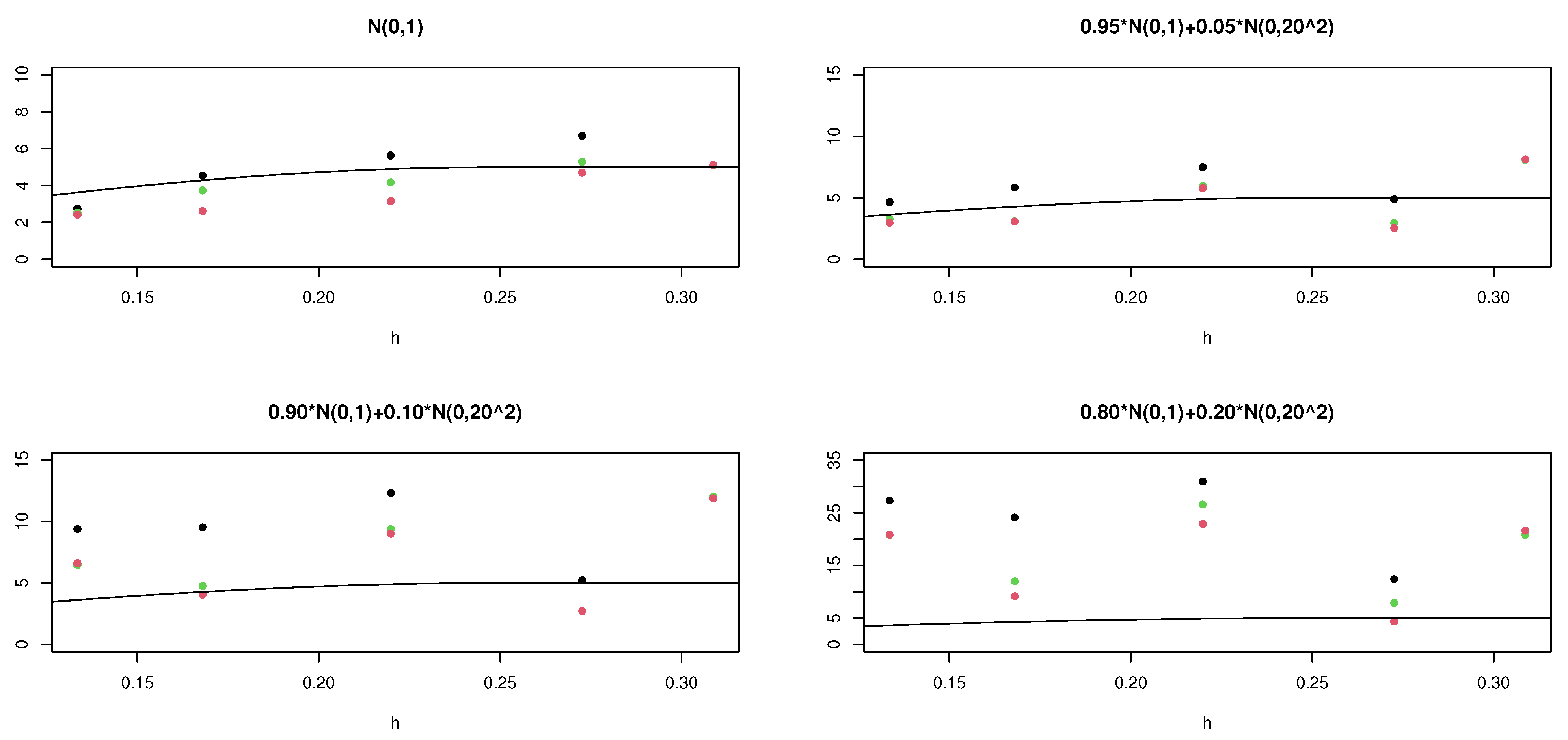
The details of the simulations are in the Supplementary Materials. In these simulations, we observe less sensitivity in the robust estimators than in the classical one, as we increase the contamination in the model. We appreciate this in Figure 4 and Figure 5. In the first one, we observe that the classical variogram model can be accepted for the three estimations in case (A), where there is no contamination. Nevertheless, as we increase the contamination (Figure 5), this variogram model does not represent the classic variogram estimations; only in some cases it represents the 0.1-trimmed variogram estimations, and it can be accepted when we consider Huber’s variogram estimations except, perhaps, in the last case, where it is doubtful.

7. Linearized Version of the Cross-Variogram Model

We saw at the end of Section 2.2 that, if linear models can be accepted as variograms and cross-variograms, the variables $X_s$ can be considered independent. These linearized versions of the model (classical and robust) were introduced in Section 9 of [5] and can be applied to model the cross-variogram. They essentially consists of replacing, before the range, the increasing part of the traditional variogram, or cross-variogram, using the regression line and, after the range, using the sill (or the robust sample mean in the robust linearized version).

Additionally, the test defined in Section 10.1 of [5] can be used to check if these models can be accepted, using saddlepoint approximations for the robust (and classical) estimators of the variograms and cross-variograms.

Namely, we test the null hypothesis of a particular variogram or cross-variogram model ${\mathcal{M}}_0(\mathbf{h})$ from which we obtain the theoretical variogram values $2{\gamma }_{ii}(\mathbf{h})$ (or cross-variogram values $2{\gamma }_{ij}(\mathbf{h})$)) using as test statistic

$$S_n=\underset{\mathbf{h}}{sup}∥2{\widehat{\gamma }}_{ii}(\mathbf{h})-2{\gamma }_{ii}(\mathbf{h})∥=\underset{1\le \left|\right|\mathbf{h}\left|\right|\le K}{max}∥2{\widehat{\gamma }}_{ii}(\mathbf{h})-2{\gamma }_{ii}(\mathbf{h})∥$$

or

$$S_n=\underset{\mathbf{h}}{sup}∥2{\widehat{\gamma }}_{ij}(\mathbf{h})-2{\gamma }_{ij}(\mathbf{h})∥=\underset{1\le \left|\right|\mathbf{h}\left|\right|\le K}{max}∥2{\widehat{\gamma }}_{ij}(\mathbf{h})-2{\gamma }_{ij}(\mathbf{h})∥$$

assuming that we consider K lags.

If we unify both as

$$S_n=\underset{\mathbf{h}}{sup}∥2\widehat{\gamma }(\mathbf{h})-2\gamma (\mathbf{h})∥=\underset{1\le \left|\right|\mathbf{h}\left|\right|\le K}{max}∥2\widehat{\gamma }(\mathbf{h})-2\gamma (\mathbf{h})∥$$

the cumulative distribution function of $S_n$ is (see [5])

$$F_{S_n}(v)=\prod _{\left|\right|\mathbf{h}\left|\right|=1}^K\left[P_{2\gamma (h)}\{2\widehat{\gamma }(\mathbf{h})>-v+2\gamma (\mathbf{h})\}-P_{2\gamma (h)}\{2\widehat{\gamma }(\mathbf{h})>v+2\gamma (\mathbf{h})\}\right]$$

probabilities that are computed with the VOM+SAD approximations.

We remark that the number K of lags (and hence the value of $\mathbf{h}$) can be modified to obtain the desired linearity.

Example 2.

Let us consider prediction data, included in the jura data set from Pierre Goovaerts’ book that contains geolocated information of several variables. This data set is calledprediction.datin the R library,gstat.

Two correlated variables, with a distribution similar to a scale contaminated normal model, are ln(Pb) (natural logarithm of Lead) and Ni (Nickel).

The values of the classical method-of-moments estimator, the 0.1-trimmed cross-variogram estimator, and the Huber’s cross-variogram estimator (with tuning constant $b=1.5$) are easily obtained for these variables, as can be seen in the Supplementary Materials. The lag distant chosen was $\mathbf{h}=0.2$. These values are shown in Figure 6.

To use their distributions, obtained in the paper, it is necessary to check if we can accept linear variograms for these two variables and a linear cross-variogram for the pair, as it was pointed out in Section 2.2. If this is the case, the variables $X_s$, $s=1,\dots ,n$ can be considered independent.

Assuming as underlying model, a scale contaminated normal with $ϵ=0.01$ and $g=1.1$, the linearized versions of the variograms for the logarithm of Lead are shown in Figure 7. The linearized versions of the variograms for Nickel are shown in Figure 8.

Finally, the linearized versions for the cross-variograms models are shown in Figure 9.

From a visual point of view, all these linearized versions can be accepted using the test considered in Section 7. The values of the test statistics $S_n={sup}_{\mathbf{h}}∥2\widehat{\gamma }(\mathbf{h})-2\gamma (\mathbf{h})∥$ and the p-values are given in

Table 3. Values of $S_n={sup}_{\mathbf{h}}∥2\widehat{\gamma }(\mathbf{h})-2\gamma (\mathbf{h})∥$ and its p-value considering a scale contaminated normal with $ϵ=0.01$ and $g=1.1$ of Example 2.

	Log Lead		Nickel		Cross-Variogram
	${\mathit{S}}_{\mathit{n}}$	p-Value	${\mathit{S}}_{\mathit{n}}$	p-Value	${\mathit{S}}_{\mathit{n}}$	p-Value
Classical	0.0704076	0.052087	27.8255	0.112065	1.160842	0.9775347
0.1-trimmed mean	0.0312044	1	58.3908	1	0.878346	0.7257757
Huber	0.0634437	1	29.0930	1	0.894193	1

(see the Supplementary Materials). Thus, the independence of the $X_s$ can be accepted.

We conclude the paper with a real-data example in which we observe how robust cross-variogram estimations provide models less sensitive to outliers, which will lead us to a more robust cokriging.

Example 3.

Let us consider the geolocated pollution data, included in the Supplementary Materials, that are the 2017 average concentrations of four air pollutants in the Community of Madrid (Spain): nitrogen monoxide (NO), nitrogen dioxide (NO₂), suspended particles with a size less than 10 microns (PM10), and ozone (O₃). These data are obtained from 22 monitoring stations [24,25,26].

Two of these 4 variables are strongly correlated and have a distribution similar to a scale contaminated normal model; they are NO and NO₂.

The variogram-crossvariogram matrix of the classical variogram and cross-variogram estimators along with classical least squares model (Mather’s model in this case) are shown in Figure 10.

The values of the classical method-of-moments estimator, the 0.1-trimmed cross-variogram estimator, and the Huber’s cross-variogram estimator (with tuning constant $b=1.5$) for these variables are obtained in the Supplementary Materials. These values are shown in Figure 11, along with the linearized cross-variogram models.

We observe that, at first lag, the three estimations agree. In the others, we can see the soft effect of the 0.1-trimmed cross-variogram and Huber’s cross-variogram estimators.

The linearized versions of the variograms and cross-variogram can be accepted, and therefore, the independence of the transformed variables $X_s$, $s=1,\dots ,n$.

Moreover, we appreciate the influence of the outliers in the estimation of the (linearized) cross-variogram in Figure 11 and, therefore, on the cokringing obtained with classical cross-variogram models. Thus, the use of robust estimators of the cross-varogram will be more reasonable in order to obtain a robust cokriging.

8. Conclusions

In this paper, we introduced new robust cross-variogram estimators and we obtained saddlepoint approximations for their distributions when the underlying model is a scale-contaminated normal distribution. We also obtained an approximation for the distribution of the method-of-moments estimator.

These approximations are especially useful when the sample size is small, a situation that we have when the size of the lag h is small.

We also proposed a suitable transformation of the initial observations to avoid the traditional dependence of the spatial observations. We see that is that linear variograms and a linear cross-variogram can be accepted as models to obtain this.

References

- Cressie NAC. Statistics for Spatial Data; John Wiley & Sons: New York, NY, USA, 1993. [Google Scholar]
- Bivand, R.S.; Pebesma, E.J.; Gómez-Rubio, V. Applied Spatial Data Analysis with R, 2nd ed.; Springer: Berlin/Heidelberg, Germany, 2013. [Google Scholar]
- Lark, R.M. Two robust estimators of the cross-variogram for multivariate geostatistical analysis of soil properties. Eur. J. Soil Sci. 2003, 54, 187–201. [Google Scholar] [CrossRef]
- Cressie, N.; Hawkins, D.M. Robust estimation of the variogram: I. J. Int. Assoc. Math. Geol. 1980, 12, 115–125. [Google Scholar] [CrossRef]
- García-Pérez, A. Saddlepoint approximations for the distribution of some robust estimators of the variogram. Metrika 2020, 83, 69–91. [Google Scholar] [CrossRef]
- Huber, P.J. Robust estimation of a locaion parameter. Ann. Math. Stat. 1964, 35, 73–101. [Google Scholar] [CrossRef]
- Tukey, J.W. A survey of sampling from contaminated distributions. In Contributions to Probability and Statistics: Essays in Honor of Harold Hotelling, Stanford Studies in Mathematics and Statistics; Oklin, I., Ed.; Stanford University Press: Palo Alto, CA, USA, 1960; Chaper 39; pp. 448–485. [Google Scholar]
- Huber, P.J.; Ronchetti, E.M. Robust Statistics, 2nd ed.; John Wiley & Sons: New York, NY, USA, 2009. [Google Scholar]
- Ebner, B.; Henze, N. Tests for multivariate normality–a critical review with emphasis on weighted L2-statistics. Test 2020, 29, 845–892. [Google Scholar] [CrossRef]
- Nadarajah, S.; Pongány, T.K. On the distribution of the product of correlated normal random variables. Comptes Rendus Math. 2016, 354, 201–204. [Google Scholar] [CrossRef]
- Daniels, H.E. Saddlepoint approximations for estimating equations. Biometrika 1983, 70, 89–96. [Google Scholar] [CrossRef]
- Withers, C.S. Expansions for the distribution and quantiles of a regular functional of the empirical distribution with applications to nonparametric confidence intervals. Ann. Stat. 1983, 11, 577–587. [Google Scholar] [CrossRef]
- Serfling, R.J. Approximation Theorems of Mathematical Statistics; John Wiley & Sons: New York, NY, USA, 1980. [Google Scholar]
- Ronchetti, E. Accurate and robust inference. Econom. Stat. 2020, 14, 74–88. [Google Scholar] [CrossRef]
- Field, C.A.; Ronchetti, E. A tail area influence function and its application to testing. Sequential Anal. 1985, 4, 19–41. [Google Scholar] [CrossRef]
- Lugannani, R.; Rice, S. Saddle point approximation for the distribution of the sum of independent random variables. Adv. Appl. Probab. 1980, 12, 475–490. [Google Scholar] [CrossRef]
- Jensen, J.L. Saddlepoint Approximations; Clarendon Press: Oxford, UK, 1995. [Google Scholar]
- Von García-Pérez, A. Mises approximation of the critical value of a test. Test 2003, 12, 385–411. [Google Scholar] [CrossRef]
- García-Pérez, A. Another look at the Tail Area Influence Function. Metrika 2011, 73, 77–92. [Google Scholar] [CrossRef]
- García-Pérez, A. A linear approximation to the power function of a test. Metrika 2012, 75, 855–875. [Google Scholar] [CrossRef]
- García-Pérez, A. A Von Mises approximation to the small sample distribution of the trimmed mean. Metrika 2016, 79, 369–388. [Google Scholar] [CrossRef]
- Field, C.A.; Ronchetti, E. Small Sample Asymptotics; Lecture Notes-Monograph Series; Institute of Mathematical Statistics: Hayward, CA, USA, 1990; Volume 13. [Google Scholar]
- R Development Core Team. A Language and Environment for Statistical Computing; R Foundation for Statistical Computing: Viena, Austria, 2020; Available online: http://www.R-project.org (accessed on 22 February 2021).
- Council-Enviroment. Department of the Madrid Environment: Air Quality Monitoring System. 2018. Available online: http://www.mambiente.munimadrid.es/opencms/opencms/calaire/consulta/descarga_\opendata.html?__locale=es (accessed on 22 February 2021).
- Council-Enviroment. Environmental Management, Council of the Environment, Local Administration and Territorial Planning, Atmospheric Quality Area-Air Quality Network. 2018. Available online: http://gestiona.madrid.org/azul_internet/html/web/2.htm?ESTADO_MENU=2 (accessed on 22 February 2021).
- Núñez-Alonso, D.; Pérez-Arribas, L.V.; Manzoor, S.; Cáceres, J.O. Statistical Tools for Air Pollution Assessment: Multivariate and Spatial Analysis Studies in the Madrid Region. J. Anal. Methods Chem. 2019, 2019, 9753927. [Google Scholar] [CrossRef] [PubMed]
Figure 1.
Approximate tail probabilities (in black) and simulated (in red) for the method-of-moments estimator with sample size , with no contamination, and with three different degrees of contamination .
Figure 2.
Tail distribution of the method-of-moments estimator with sample size and two underlying models: and , for three different degrees of contamination .
Figure 3.
Tail probabilities of the classical method-of-moments cross-variogram estimator (top row of figures) and -trimmed cross-variogram estimator (bottom row of figures), with no contamination, , and contaminations and .
Figure 4.
Variogram estimations of Example 1: classical (black), 0.1-trimmed (green) and Huber’s (red), and the variogram model with no contamination.
Figure 5.
Figure 6.
Classical (black) and robust (green and red) cross-variogram estimations of Example 2.
Figure 7.
Classical (black) and robust (green and red) variogram estimations for the logarithm of lead and their linearized variograms of Example 2.
Figure 8.
Classical (black) and robust (green and red) variogram estimations for nickel and their linearized variograms of Example 2.
Figure 9.
Classical (black) and robust (green and red) cross-variogram estimations, linearized versions, and the classical model (blue) of Example 2.
Figure 10.
Variogram-crossvariogram matrix of the classical variogram and cross-variogram estimations with the classical model of Example 3.
Figure 11.
Classical (black) and robust (green and red) cross-variogram estimations of Example 3, with the linearized cross-variogram models.