Functional Symmetry and Statistical Depth for the Analysis of Movement Patterns in Alzheimer’s Patients

Abstract

Black-box techniques have been applied with outstanding results to classify, in a supervised manner, the movement patterns of Alzheimer’s patients according to their stage of the disease. However, these techniques do not provide information on the difference of the patterns among the stages. We make use of functional data analysis to provide insight on the nature of these differences. In particular, we calculate the center of symmetry of the underlying distribution at each stage and use it to compute the functional depth of the movements of each patient. This results in an ordering of the data to which we apply nonparametric permutation tests to check on the differences in the distribution, median and deviance from the median. We consistently obtain that the movement pattern at each stage is significantly different to that of the prior and posterior stage in terms of the deviance from the median applied to the depth. The approach is validated by simulation.

1. Introduction

Alzheimer’s disease is a neurodegenerative condition that affects 15 million people worldwide [1]. The evolution of the patient passes through different stages of the disease, which, according to the Global Deterioration Scale (GDS) [2], are:

(GDS 1)

no cognitive impairment,

(GDS 2)

early cognitive impairment,

(GDS 3)

mild cognitive impairment,

(GDS 4)

mild dementia,

(GDS 5)

moderate dementia,

(GDS 6)

moderately severe dementia and

(GDS 7)

severe dementia.

An important aspect is diagnosing when a patient evolves from his or her current stage into the next one, which usually entails a complex physical examination carried by the patient’s medical doctor. As an additional tool for the doctor to consider in taking that decision, [3,4] analyzed the movement patterns of Alzheimer’s sufferers when moving freely in a daycare facility. The objective of those papers was supervised classification, so that given the movement patterns of a set of patients and their disease stage, the stage of other patients could be predicted based on their movement patterns. The analysis used neural networks applied to multivariate time series data. This is a black-box technique that results in high success rates, 83% in [4] and 91% in [3], but does not reveal which characteristics of the data helped with the classification. In [4], also an attempt to analyze the data as functional data was made. However, no significant findings were obtained that way.

The analyzed real data are recordings made by the accelerometer device of an Android smartphone with a sampling rate of 8 Hz. These acceleration forces are measured in the three spatial dimensions over time while the patients carry the smartphone in their pocket. The data comprise repeated trivariate measurements on 35 patients in different stages of Alzheimer’s disease:

• 7 patients in a mild stage of the disease (GDS 2 and 3),
• 18 patients in a moderate stage of the disease (GDS 4 and 5) and
• 10 patients in a severe stage of the disease (GDS 6 and 7).

The data are unusually complex in that the number of repeated measurements is different for each patient, between 2 and 8, with a total of 187 measurements (187 three-dimensional curves). Moreover, the length of the domain over which the trivariate functional data are observed is different for each measurement and the grid of discretization points is also different for each measurement.

This type of data is functional in nature, in fact, it can be viewed as longitudinal functional data [5]. The modern research theme of functional data analysis (FDA) [6,7], in which collections of measurements are viewed as partially observed realizations of random functions (a natural viewpoint for e.g., growth trajectory data, brain imaging data and handwriting data), belongs primarily to the area of non-parametric statistics and will allow us to further develop the analysis of these data from an exploratory perspective. This will provide information for a more interpretable model, in contrast to the widespread black-box approaches to classification. For this, we will use the concepts of statistical symmetry [8] and data depth [9].

Statistical depth functions provide an order for the elements of a given space $\mathcal{X}$ by making use of a probability distribution P on that space. The deepest element(s) are generally referred to as the median, coinciding with the center of symmetry of P when a unique center of symmetry exists for some notion of symmetry. Although providing an order in spaces of dimension higher than one is a non-trivial task, it is important because statistics of order are the basis of many established nonparametric procedures, for instance, inference based on ranks and the detection of outliers. Outlier detection is a necessary preliminary stage in many statistical investigations and inference based on ranks can be used, for example, in supervised classification and clustering.

Just as in the case of $\mathcal{X}={\mathbb{R}}^p$, there is no unique definition of symmetry when $\mathcal{X}$ is a function space $\mathcal{F}$. Thus, in Section 2, we discuss difficulties associated with some potential notions of symmetry for distributions on $\mathcal{X}=\mathcal{F}$ and show there are situations whereby a distribution on a functional space would be deemed symmetric with respect to several of these notions, despite possessing important topological asymmetries. After highlighting such difficulties, we describe the notion of functional symmetry used to explore the Alzheimer’s dataset. Simultaneously, we will explain the complexity involved in defining a statistical functional depth and give details of the one relevant for our application, which allows for multivariate functional data. It will require specification of an appropriate metric space and the aforementioned notion of functional symmetry. In Section 3, we perform a simulation to illustrate that the notion of functional symmetry employed is preserved through the use of derivatives. This is important as the acceleration is the second derivative of the position with respect to the time. Section 4 provides the data analysis and a suitable metric space for it. We finalize with a discussion in Section 5.

2. Methodology

2.1. Symmetry

Symmetry is a fundamental concept, and has been the focus of much contemplation throughout history due to its manifestation in natural and scientific phenomena, as well as in man-made structures. Its usage is common in modern language as a means to express a particular type of structure or regularity, often geometric, that of exact correspondence between parts of an object with reference to a point or axis of symmetry. Typically though, the mathematical formalization of symmetry entails invariance under a family of measurable transformations [10]. In simple geometric contexts, this might be invariance under sign changes or under rotation.

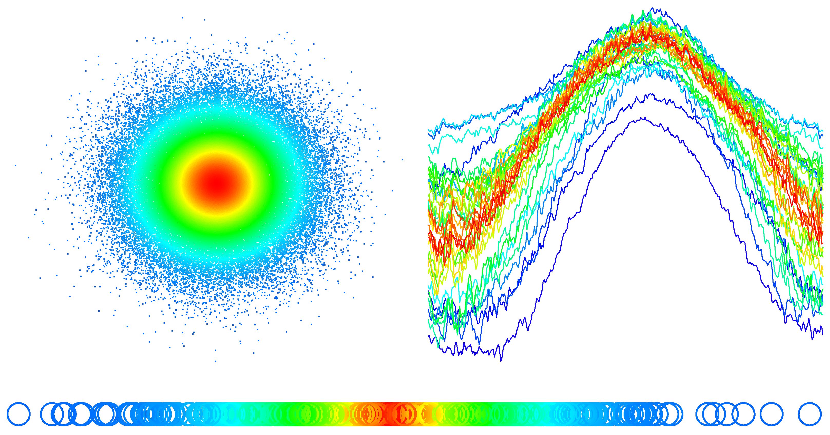
We focus on symmetry in statistics, in this case, it is not the random objects themselves to which a notion of symmetry applies, but rather their distributions. In Figure 1, essential features of a symmetric probability distribution P are depicted, for: a space of dimension one, $\mathcal{X}=\mathbb{R}$; a multivariate space, $\mathcal{X}={\mathbb{R}}^p$; and space of functions, $\mathcal{X}=\mathcal{F}$. We explain in detail the concept of depth later in the manuscript; however, it is worth saying that, in the figure, symmetries in the distribution with respect to an element $\zeta$ of $\mathcal{X}$ are discernible in the color, with $\zeta$ the center of symmetry. In fact, the changes in the colors show that the datasets are ordered from the center outward.

2.1.1. Difficulties with Notions of Functional Symmetry

The intangibility of distributions on function space leads to great difficulties in formulating a well conceived notion of symmetry in this domain, as naïve point-wise extensions of familiar notions in $\mathbb{R}$ or ${\mathbb{R}}^p$ ignore topological features such as continuity, contiguity and smoothness. We illustrate the difficulties in formulating a notion of functional symmetry through a prototypical example of a distribution on function space, asymmetric by construction, but symmetric with respect to many topologically apathetic notions of functional symmetry.

For that, we make use of ([11], Example 2) where X denotes a mixture of three processes on $[0,1],$ with probabilities $p_1=0.2$, $p_2=0.3$ and $p_3=0.5$, each following a mean zero Gaussian distribution. They differ according to the correlation length parameter m in their covariance structure:

$$\mathrm{Cov}(s,t)=e^{-\frac{{(s-t)}^2}{2m^2}},$$

where $m\in \{1,0.25,0.1\}$.

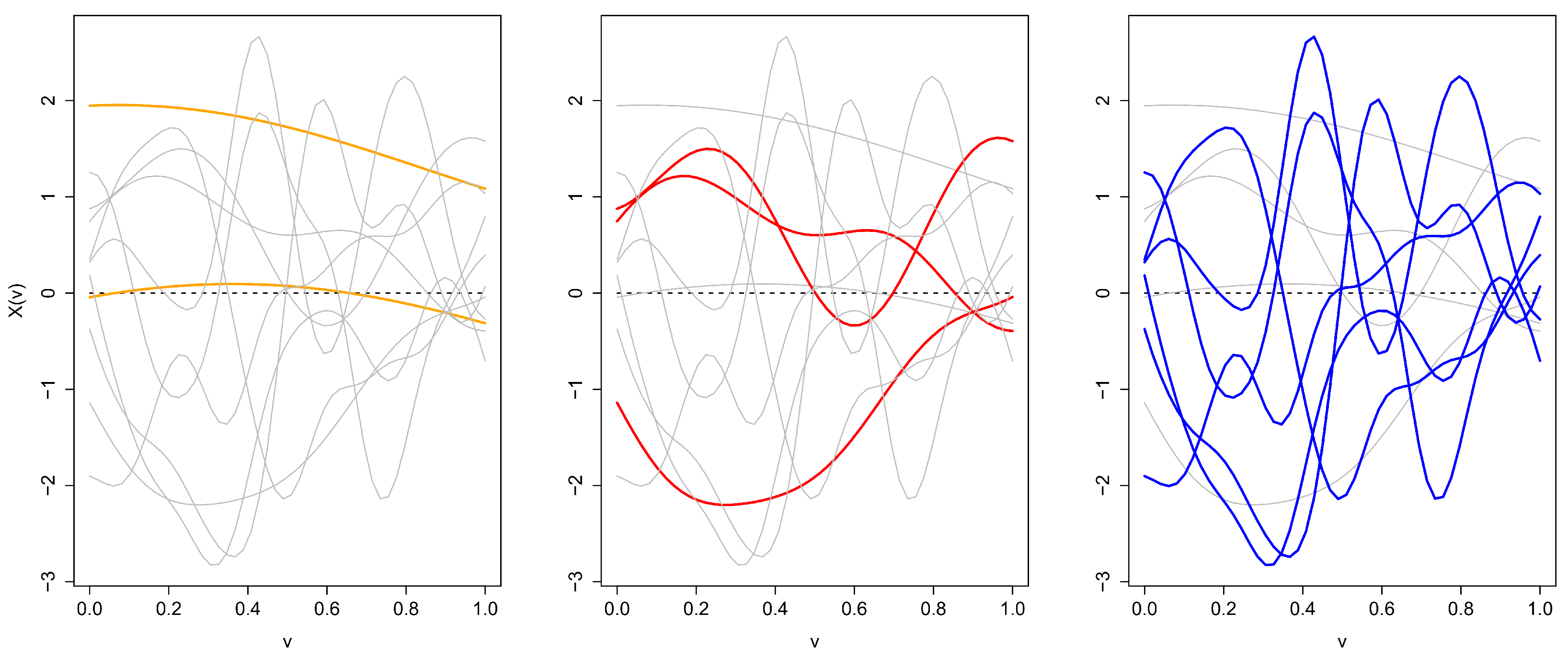
Figure 2 depicts $n=11$ typical realizations of this process, with the different panels emphasizing the elements of the sample corresponding to the different correlation lengths. A symmetry notion exclusive for spaces of functions should naturally consider topological characteristics, for instance, shape and roughness. Note the difference among the three processes in the mixture by observing the differences in the curves of the three panels of Figure 2, from those with less curvature on the left to those with more curvature on the right. Thus, by making use of an appropriate metric on the functional space, the notion of symmetry we will apply here correctly recognizes that mixtures of Gaussian distributions like X are asymmetric.

However, X is clearly symmetric around the zero function for several extensions of multivariate symmetry; for example:

(i)

X and $-X$ are equal in law,

(ii)

for any $v \in$ [0, 1], the distribution of $X\left(v\right),$ or of its derivative at $v,$ is symmetric on $\mathbb{R}$ around zero and

(iii)

for any reasonable notion of symmetry in multivariate spaces, any finite linear combination of the random coefficients in the Karhunen-Loève expansion [12] of the process $X,$ or of its derivative process, is symmetric around the zero element.

There is no inconsistency between X not being functional symmetric and being symmetric with respect to plausible extensions of multivariate notions. The notions are complementary. If the mixture of Gaussian distributions is asymmetric in terms of shape or roughness, there should be a type of symmetry that is sensitive to this, as described below.

2.1.2. Metric $\delta$-Symmetry

The notion of symmetry employed in this paper was recently defined in [11] and is suitable for any function space, $\mathcal{F},$ endowed with a metric, or pseudo-metric, which we denote by $d.$ For any fixed $\delta \in [0,\infty ),$ a distribution P on $\mathcal{F}$ with support $\mathfrak{S}$ is $(d,\delta )$-symmetric about a center

$$\zeta \left(\delta \right):=\zeta (\delta ,P)\in \mathfrak{S}$$

if

$$P\left({\mathfrak{H}}_x^{\zeta \left(\delta \right)}\right)\ge 0.5-\delta$$

for all $x\in \mathfrak{S}$, with

$${\mathfrak{H}}_x^{\zeta \left(\delta \right)}:={\mathfrak{H}}_x^{\zeta \left(\delta \right)}\left(P\right)=\{z\in \mathfrak{S}:d(z,x)\ge max[d\{x,\zeta \left(\delta \right)\},d\{z,\zeta \left(\delta \right)\}]\}.$$

Denoting,

$$\mathcal{Z}\left(\delta \right):=\mathcal{Z}(\delta ,P)=\{z\in \mathfrak{S}:P\left({\mathfrak{H}}_x^z\right)\ge \frac{1}{2}-\delta \mathrm{for}\mathrm{all}x\in \mathfrak{S}\},$$

(1)

we have that any

$$\zeta \left(\delta \right)\in \mathcal{Z}\left(\delta \right)$$

is a center of $(d,\delta )$-symmetry of the space $\mathcal{F}$ with respect to the distribution P.

The $(d,\delta )$-symmetry induces a functional median of the space $\mathcal{F}$ with respect to the distribution P, the metric median, which is

$$\mathcal{M}\left(P\right):=arg\underset{z\in \mathfrak{S}}{min}\{\delta \in [0,\infty ):P\left({\mathfrak{H}}_x^z\right)\ge \frac{1}{2}-\delta \mathrm{for}\mathrm{all}x\in \mathfrak{S}\}.$$

A distribution on a metric function space is generally understood as symmetric if it is $(d,0)$-symmetric. The $\delta$ for which $M\left(P\right)$ is obtained when being larger than 0 is the degree of departure from $(d,0)$-symmetry. As it occurs with the median in $\mathbb{R},$ a center of $(d,\delta )$-symmetry is not necessarily unique (as observable from Equation (1)). Additionally, it is functional affine invariant and has a consistent and qualitatively robust sample version [11].

This definition of symmetry shares some common ground with the notion of multivariate half-space symmetry in that both notions are generalizations of Equation (2) below. Half-space symmetry is introduced in [8] for distributions on ${\mathbb{R}}^p$, as a means to generalize the previously existing notions of multidimensional symmetry such as central symmetry and angular symmetry. In the particular case of $p=1$, according to [8] a distribution P on $\mathbb{R}$ is half-space symmetric about a center $\zeta$ if

$$P\left(H_x^{\zeta }\right)\ge \frac{1}{2}$$

for all $x\in \mathbb{R}\backslash \zeta ,$ with

$$H_x^{\zeta }:=\left\{z\in \mathbb{R}:|z-x|\ge max\left\{\right|x-\zeta |,|z-\zeta \left|\right\}\right\}.$$

(2)

An important point illustrating the generality of $(d,\delta )$-symmetry, and equivalently of half-space symmetry, is that, in this special case of $p=1$, all distributions are $(d,0)$-symmetric with center of symmetry at the median, despite not necessarily being so with respect to more geometrically intuitive notions of symmetry.

The concept of $(d,\delta )$-symmetry is the first one designed specifically for functional data. Apparently, it could be applied to any metric space, however, it is indeed exclusive to functional data in the sense that it has no useful analogue in a multivariate context. This can be deduced from the reasoning in Section 2.1.1.

2.2. Statistical Depth

Just as in other disciplines, symmetry is a recurrent theme in statistics. For instance, symmetric laws frequently arise as limit laws of empirical processes [13,14], and, as we have just seen, the notion of symmetry helps to generalize the concept of median beyond the one dimensional case, for which it has a simple and unambiguous definition. In addition to being of independent interest, a notion of symmetry is required for constructing statistical depth functions, as is clear from the property based definition of depth appearing in [9,15]. According to this definition, the deepest element in a space $\mathcal{X}$ computed with respect to a distribution P on $\mathcal{X}$ coincides with the center of symmetry of P when a unique center of symmetry exists for some notion of symmetry. The other properties in this definition are: distance invariance, strictly decreasing with respect to the deepest element, upper semi-continuity, receptivity to convex hull width across the domain and continuity in distribution.

Loosely speaking, statistical depth orders the elements of a space with respect to a distribution, or a dataset (an empirical distribution). Thus, it lays the foundation for many nonparametric and exploratory data analysis tools such as rank-based inference and outlier detection, whose potential applications are wide ranging. We will employ statistical functional depth here as an exploratory tool to gain insight into the movement patterns of Alzheimer’s patients.

2.2.1. Difficulties with Functional Depth Constructions

Refs. [16,17] report a problematic feature of certain depth constructions, both multivariate depths (half-space [18], simplicial [19], projection [9]) and functional depths (band [20], half region [21]). This feature is their degenerate behavior when applied in some common functional spaces. Therefore, in formulating a functional depth, it does not suffice to simply extend the finite dimension to infinity. The literature contains several instances of functional depth (h-depth [22], random Tukey depth [23,24], modified band depth [20], modified half region depth [21], spatial depth [25], for instance) and an axiomatic definition of functional depth put forward in [15]. However, the above cited commonly used proposals violate at least one of these axioms.

Recently, Ref. [11] has given a functional depth construction designed for functional metric spaces, and not multivariate. This construction was proved to satisfy the axiomatic definition of statistical functional depth under a mild condition on the metric. That condition is met by most metrics, including the Lebesgue and Sovolev metrics, but not the supremum metric. The construction, which we describe below, makes use of the set of centers of $(d,\delta )$-symmetry. As a result of the relation of this set with the multivariate half-space depth median, a depth that suffers from the problem reported in [17], one might expect it to inherit this degeneracy. However the non-vanishment of the half-space depth median ([17], Theorem 3) guarantees that this is not the case.

2.2.2. Metric Depth

Given a $(d,\delta )$-symmetric distribution P on a functional metric space $(\mathcal{F},d)$, with $\mathcal{Z}$ the set of centers, the metric depth of an element x of $\mathcal{F}$ with respect to a distribution P is defined in [11] as

$$D_m(x,P):=\frac{1}{I_m(x,P)+1}$$

(3)

with

$$I_m(x,P):=\frac{d(x,\mathcal{Z})}{d(\xi ,{\xi }^{\prime })}:=\underset{\zeta \in \mathcal{Z}}{inf}\frac{d(x,\zeta )}{d(\xi ,{\xi }^{\prime })}$$

(4)

and

$$\xi :=\xi \left(P\right)\mathrm{and}{\xi }^{\prime }:={\xi }^{\prime }\left(P\right)\in \mathcal{F}$$

satisfying $d(\xi ,{\xi }^{\prime })>0$ and independent of $x.$

This depth function computes the distance of the element of the space to the set of centers of functional symmetry and then standardizes so that the axiomatic properties in [15] are satisfied, under a mild condition on the metric. This is a general framework to be specified through the distance, for instance:

(i)

A distance that makes use of the distribution with respect to which the depth is computed. In the space of continuous functions, the distance between two elements of the space can be defined through the probability of the band determined by them.

(ii)

A Sobolev distance that takes into account how rough the datum is with respect to the functional center of symmetry.

In the context of the Alzheimer’s data, it suffices to make use of

$$I_M(x,P):=d(x,\mathcal{Z}):=\underset{\zeta \in \mathcal{Z}}{inf}d(x,\zeta )$$

(5)

in (3) instead of (4) because, given $P,$ $d(\xi ,{\xi }^{\prime })$ is constant for every x in the space, (see [11]).

3. Illustration

The dataset of Alzheimer’s patients, analyzed later, consists of the accelerations recorded by the accelerometer of an Android smartphone while the patients move freely in a daycare facility. On exploring this dataset, we aim to study whether the underlying distribution generating the data is symmetric. The acceleration is the derivative of the velocity with respect to time, which, as well, is the derivative of the position with respect to time. Accelerometers provide directly the acceleration, without the need for differentiating the data. However, in studying the distribution underlying the movement of Alzheimer’s patients, it is relevant that symmetries are perpetuated through derivatives, particularly, the first and the second.

We provide an example to illustrate that the notion of symmetry we use has the distinctive feature of inducing symmetry in other domains. Let X denote a Gaussian process with mean zero, covariance structure

$$\mathrm{Cov}(s,t)=e^{-\frac{{(s-t)}^2}{m^2}}$$

and correlation length $m=1$ and $X_1,\dots ,X_n$, $n=1000$ independent realizations drawn from $X.$

For $i=1,\dots ,n$, we plot

$$\int (X_i-\zeta )\left(v\right)dv$$

versus

$$\int (X_i^{\left(1\right)}-{\zeta }^{\left(1\right)})\left(v\right)dv$$

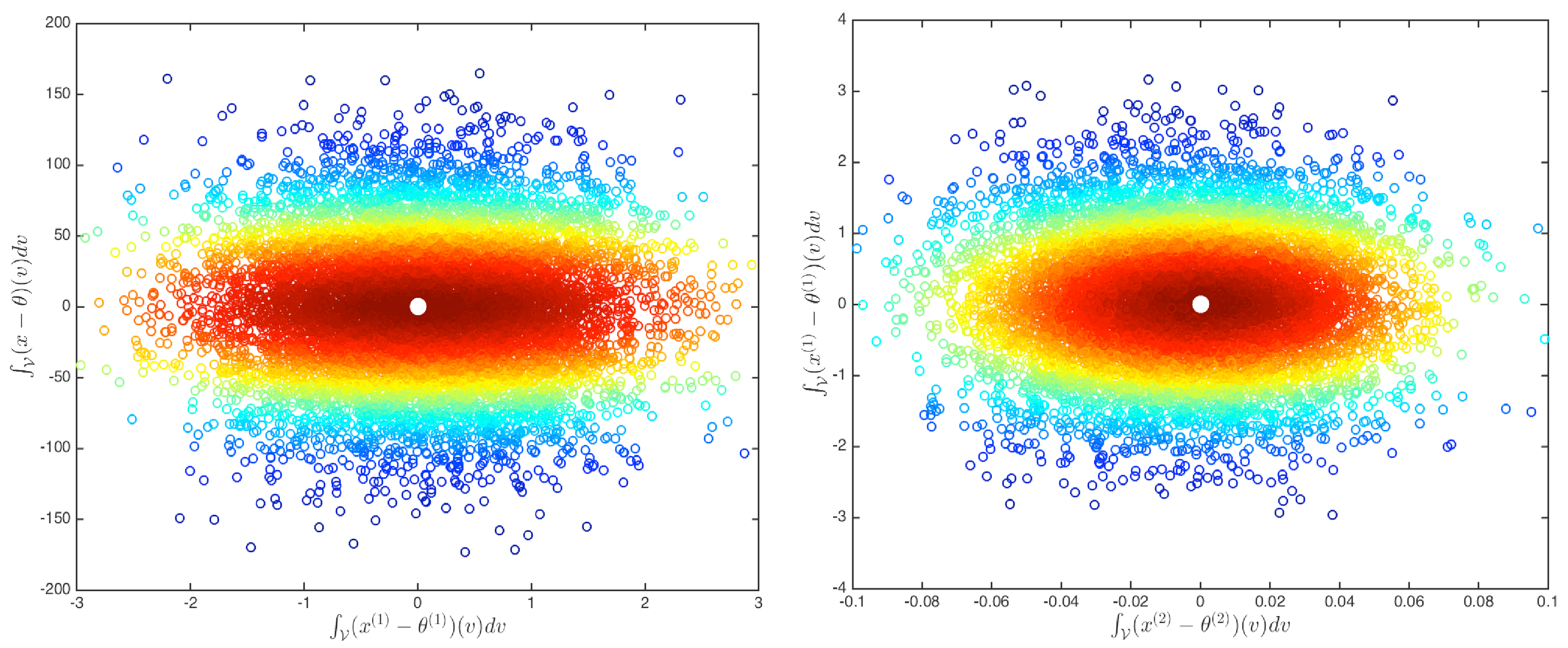
in the left plot of Figure 3 and

$$\int (X_i^{\left(1\right)}-{\zeta }^{\left(1\right)})\left(v\right)dv$$

versus

$$\int (X_i^{\left(2\right)}-{\zeta }^{\left(2\right)})\left(v\right)dv$$

in the right plot of Figure 3. There, $X_i^{\left(j\right)}$ denotes the jth derivative of $X_i$, for $j=1,2$ and $i=1,\dots ,1000$.

To illustrate that our notion of symmetry has the distinctive feature of inducing symmetry in these two domains, we compute the set of sample centers of $(d,0)$-symmetry based on the empirical distribution of $X_1,\dots ,X_{1000}$, $P_n$, and the corresponding metric depth of $X_i$ with respect to $P_n$ for each $i=1,\dots ,n$. We depict in Figure 3 the center of symmetry as a white dot and the metric depth of each point by the color (from dark red for high depth to dark blue for low depth).

Let us denote by ${\mathbb{L}}_2$ the standard Lebesgue 2-integrable norm and by Sobolev-(2,k) the standard Sobolev inner product norm for k derivatives. To illustrate the importance of taking into account the topology of the elements in the support of the distribution, we use the Sobolev-(2,2) distance for the left panel of the figure and the Sobolev-(2,2) distance minus the ${\mathbb{L}}_2$ distance for the right panel. Thus, the colors in the right panel, given by the center and depth, only make use of a distance based on the first and second derivatives.

4. Application

As mentioned in the introduction, the dataset consists of the acceleration values, in the three spatial dimensions over time, of patients that move freely in a daycare facility. Although non-standard, these data are easily accommodated by the $(d,\delta )$-symmetry and the metric depth as shown below in Section 4.1. We make use of nonparametric tests on the depth results as described in Section 4.2 and evaluate this methodology through Monte Carlo simulations in Section 4.3. Section 4.4 summarizes and explains the real data we analyze. The results of such analysis are in Section 4.5.

4.1. Functional Metric Space Construction

We denote by n the total number of studied patients and by $x_i$ the acceleration values recorded for patient i, $i=1,\dots ,n$. As the accelerations of each patient were recorded in separate days, we have repeated measurements for each patient, we denote by $k_i$ the number of repeated measurements for patient i and by $x_{i1},\dots ,x_{i{k}_i}$ the repeated measurements, $i=1,\dots ,n$. We later refer to these repeated measurements as repetitions. Thus,

$$x_i=(x_{i1},\dots ,x_{i{k}_i})\mathrm{for}i=1,\dots ,n.$$

(6)

As each measurement is a three dimensional functional datum, we have that

$$x_{ik}:[l_{ik},u_{ik}]\to {\mathbb{R}}^3$$

is the kth measurement on patient i and

$$L\left(x_{ik}\right):=u_{ik}-l_{ik}$$

is the length of the domain. A particularity of this dataset is that the domain, $[l_{ik},u_{ik}]$, and its length, $L\left(x_{ik}\right)$, differ for each $k=1,\dots ,k_i$ and $i=1,\dots ,n$. This requires non-standard FDA methodologies like the ones we apply here.

A characteristic of real functional data is that they are observed on a grid, not being recorded in every point of the domain. That is, $x_{ik}\left(t\right)$ is not recorded at each $t\in [l_{ik},u_{ik}]$, but at each t in the finite set

$${\mathcal{T}}_{i,k}:=\{t_{1,i,k},\dots ,t_{T_{i,k},i,k}\}$$

with

$$l_{ik}\le t_{1,i,k}<t_{2,i,k}<\cdots <t_{T_{i,k},i,k}\le u_{ik},$$

not necessarily equally spaced. Part of the complexity of this dataset is that ${\mathcal{T}}_{i,k}$ differs for each $k=1,\dots ,k_i$ and $i=1,\dots ,n$.

The $(d,\delta )$-symmetry and the metric depth require of a metric functional space for their application. Then, given any pair $(x_{ik},x_{j\ell })$ with $k\in \{1,\dots ,k_i\}$, $\ell \in \{1,\dots ,k_j\}$ and $i,j\in \{1,\dots n\}$, we define our distance between $x_{ik}$ and $x_{j\ell }$ as

$$d_S(x_{ik},x_{j\ell }):=max\{d\left(x_m,x_M\left({\mathcal{V}}_h\right)\right):h\in [0,L\left(x_M\right)-L\left(x_m\right)]\}$$

(7)

where the notation $x_i\left(\mathfrak{S}\right)$ means $\left\{x\right(t):t\in \mathfrak{S}\}$ and, additionally,

$$x_m:=argmin\{L\left(x_{ik}\right),L\left(x_{j\ell }\right)\},$$

$$x_M:=argmax\{L\left(x_{ik}\right),L\left(x_{j\ell }\right)\}$$

and ${\mathcal{V}}_h$ is such that

$$x_M\left({\mathcal{V}}_h\right)=\{x_M\left(t\right):0\le t-l_M-h\le L\left(x_m\right)\}.$$

It is easy to see that $d_S(·,·)$ satisfies the definition of a distance, for any distance d. In the data analysis, for two three dimensional functional data objects

$$f=\{f_1,f_2,f_3\}$$

and

$$g=\{g_1,g_2,g_3\},$$

which are defined over the same domain, we take

$$d(f,g)=1/3\sum _{i=1}^3\parallel f_i-g_i\parallel ,$$

(8)

where $\parallel ·\parallel$ is a norm, for instance the ${\mathbb{L}}_2$ norm. We then aggregate the information from the repeated measurements as

$$\frac{1}{k_i{k}_j}\sum _{k=1}^{k_i}\sum _{\ell =1}^{k_j}{d}_S(x_{ik},x_{j\ell }),$$

and use this to construct the set of centers of $(d,\delta )$-symmetry and the metric depth as described previously.

4.2. Tests on the Statistical Depth Values

The dataset consists of patients at three different stages of the disease and the analysis will provide a depth value for each. Let

$$D_m:=\{D_{m,1},\dots D_{m,l_m}\}$$

be the depth values for the patients in a mild stage of the disease,

$$D_o:=\{D_{o,1},\dots D_{o,l_o}\}$$

the depth values for those in a moderate stage and

$$D_s:=\{D_{s,1},\dots D_{s,l_s}\}$$

the depth values for those in a severe stage. Abusing of the notation, $D_m$, $D_o$ and $D_s$ will stand also for the corresponding depth random variables. Note that $l_m+l_o+l_s=n$. We will illustrate the methodology using $D_m$ and $D_o$. Analogous ideas apply to all combinations of depths for mild, moderate and severe disease stages.

Depth values have an inherent rank structure. To test for differences between the distributions of the trivariate acceleration functions, we apply two sided nonparametric tests to the associated depth values. One of them is an omnibus test, a test that can potentially pick any difference between two distributions with independence of the nature of the difference. It is also important to know where the differences lie. Thus, we propose to perform two further tests, one on the median differences and another on the scale differences. The scale test is a test on the deviance from the median [26]. We do them on the median, as opposed to the mean, in order to perform non-parametric robust tests. These last two tests have hypotheses of the form

$$\begin{array}{cc}{H}_0:& {\mathfrak{p}}_m\le {\mathfrak{p}}_o\\ H_a:& {\mathfrak{p}}_m>{\mathfrak{p}}_o,\end{array}$$

where ${\mathfrak{p}}_m$ refers respectively to the population median and the deviance from the population median in the mild group and ${\mathfrak{p}}_o$ is the same parameter in the moderate group.

Given $D_m$ and $D_o$ and a statistic G, all of these tests are permutation tests [27] of the following form:

• Compute the value of the statistic on the observed depth values

  $$g_{obs}:=G(D_m,D_o).$$
• Compute the permutations of the $l_m+l_o$ depth values between two groups, one with $l_m$ elements and the other with $l_o$. There is a total of

  $$N:=(l_m+l_o)!/(l_m!l_o!)$$

  permutations.
• Compute the value of the statistic on each of the permutations, $g_1,\dots ,g_N.$
• The resulting p-value for the test is

  $$p:=\#\{i=1,\dots ,N:g_i\ge g_{obs}\}/N.$$

For the omnibus test, we apply the Kolmogorov–Smirnov test [28,29] to the depths. The associated test statistic is

$$G_{KS}(D_m,D_o):=\underset{t\in \mathbb{R}}{max}|F_{D_m}\left(t\right)-F_{D_o}\left(t\right)|,$$

where $F_D\left(t\right)$ is the cumulative distribution of D at time t. As $G_{KS}$ involves an absolute value, performing the above steps for the permutation test will result in this case on a test for the null hypothesis of equality of distributions against the distributions being different. For the test on the median differences, the test statistic is

$$G_M(D_m,D_o):=\mathrm{Med}\left(D_m\right)-\mathrm{Med}\left(D_o\right),$$

where $\mathrm{Med}\left(D\right)$ denotes the median of D. For the deviance from the median test, the statistic is

$$G_S(D_m,D_o):=\frac{{\displaystyle \sum _{i=1,\dots ,l_m}|D_{m,i}-\mathrm{Med}\left(D_m\right)|}}{{\displaystyle \sum _{i=1,\dots ,l_o}|D_{o,i}-\mathrm{Med}\left(D_o\right)|}}.$$

4.3. Simulation

We perform a Monte Carlo study to evaluate the performance of the methodology described above. The following simple example was used for illustration in ([11], Example 1). Functional random variables X are generated as

$$X\left(t\right)=Ycos\left(\pi t\right)$$

with Y a real random variable and $t\in [0,1].$ As studied in [11], the distribution of X is $(d,0)$-symmetric independently of d and the choice of distribution for Y. To emulate the different populations of patients in the Alzheimer’s data, we generate observations $X_{m,1},\dots ,X_{m,l_m}$ from one population, Population m say, by taking Y to be standard normally distributed. We generate, independently, observations $X_{o,1},\dots ,X_{o,l_o}$ from Population o by drawing Y from a distribution Q, taken in turn as standard normal, standard uniform and beta of parameters 2 and 1. We use of a grid of 50 equi-spaced points on $[0,1]$ and, to emulate the Alzheimer’s data, we take $l_m=l_o=10$.

For the analysis, we use the metric depth, based on the set of (d,0)-centers of symmetry, with respect to the pooled sample with d taken as the Sobolev-(2,2) distance; obtaining the depth values $\{D_{m,1},\dots D_{m,l_m}\}$ and $\{D_{o,1},\dots D_{o,l_o}\}$. We then apply the methodology described in Section 4.2 to these depth values. When Q is the standard normal distribution, the distributions of $X_{m,j}$ and $X_{o,i}$ are the same for any i and j and we expect the tests to reject infrequently. Specifically, we expect the proportion of rejections over the Monte Carlo replications to be roughly equal to the nominal level of the test. When Q is one of the other distributions, the proportion of rejections will ideally be large, as this indicates strong ability to distinguish between distributions of the functional random variables on the basis of their functional depth values.

The median and deviance from the median tests used are exact permutation tests. As the distribution test has more computational cost, we have performed an approximated permutation test based on 1000 permutations. The proportion of Monte Carlo replications in which the test rejects the null hypothesis of equal distributions is reported in

Table 1. Rate of rejection based on 1000 repetitions for three permutation tests: distribution, median and deviance from the median. The permutation tests for the median and deviation from the median are exact. The permutation test for the distribution is approximated, based on 1000 permutations. The first sample is based on the standard normal distribution, N(0,1), and the second on the N(0,1) (first column), the uniform in the (0,1) interval, U(0,1), (second column) and the beta with parameters (2,1), $\beta$(2,1), (third column).

	N(0,1)	U(0,1)	$\mathit{\beta }$(2,1)
Distribution	0.034	0.591	0.749
Median	0.053	0.795	0.891
Deviance	0.042	0.801	0.913

for each of the three scenarios. It is observable from the table that the power of rejection is higher when the $X_{o,i}$s are drawn using the beta distribution with parameters (2,1) than when using the uniform distribution. Additionally, under the alternative, the deviance from the median test is more powerful than the median test, which is also more powerful than the distribution test. The low rejection rate of the distribution test under the null hypothesis can be due to an approximated permutation test is performed.

4.4. The Data

The real data were measured in the patients’ natural environment rather than a controlled environment as in [30]. Patients’ movements were recorded while they perform their usual activities throughout the day under the supervision of a neuropsychologist, in a room of a day care facility. The smartphone is oriented and placed in a pocket of the patient by the neuropsychologist. Thus, the orientation and placement of the smartphone is never exactly the same, neither among patients nor among the different days in which the accelerations of a particular patient are recorded.

From a purely statistical point of view, it is always advantageous to use data from a controlled experiment. However, for the statistical classifier to be a valuable and widely applicable diagnostic tool, it is necessary to use observational data of the type studied here. Ref. [31] asserts that the everyday behavior of Alzheimer’s patients is detectable by using only an accelerometer, without the need for an additional gyroscope for standardization. For a more detailed discussion, see [4], where these data were first analyzed.

The study comprises data on $n=35$ patients for whom repeated measurements are available corresponding to different days. The repetitions $k_i$ in (6), vary between 2 and 8 depending on the patient labeled as $i=1,\dots ,n$. The value of $k_i$, for each i, is displayed in Table 2, column two, under the heading repetitions. There, the disease stage of each patient is also shown in column three. The information obtained from these two columns is summarized in Table 3, from which we observe that:

• 7 patients are in the mild stage of the disease with a total of 41 repetitions.
• 18 patients are in the moderate stage of the disease with a total of 100 repetitions.
• 10 patients are in the severe stage of the disease with a total of 46 repetitions.

Table 2. Synopsis of the studied dataset. For each of the 35 patients (column i), labeled from 1 to 35, it is displayed the number of repeated measurements (column ii), the disease stage of the patient (column iii), the range, among the repetitions for each patient, of the time domain upper-bounds, in seconds, (column iv) and the range, among the repetitions for each patient, of the number of grid points (column v).

Patient	Repetitions	Disease Stage	Maximum Range	Grid Range
1	5	moderate	3273.8–4149.3	457,352–574,918
2	3	severe	2721.6–3573.2	380,756–493,117
3	3	mild	3077.8–3679.8	426,027–508,825
4	6	mild	3168.5–3847.7	447,858–542,706
5	5	severe	2786.6–4109.3	396,699–583,914
6	3	severe	3356.4–3587.0	469,298–498,984
7	7	severe	2993.3–3878.0	426,625–545,839
8	8	mild	2610.7–3778.1	366,541–531,256
9	3	severe	3419.6–3633.7	474,456–500,270
10	6	moderate	3090.3–3952.5	427,229–547,061
11	8	mild	2718.5–3870.4	267,288–385,509
12	5	moderate	3069.8–4112.8	257,796–388,149
13	8	moderate	2802.8–5003.5	245,309–520,520
14	7	severe	3365.1–5942.7	327,976–560,693
15	7	mild	3590.9–4127.8	295,551–344,340
16	7	severe	3472.2–5452.3	327,583–496,692
17	4	mild	3405.0–4008.7	182,260–295,130
18	6	moderate	3168.1–4068.7	211,480–389,936
19	5	mild	3189.9–3667.0	298,743–339,375
20	7	moderate	2765.9–4469.5	259,898–354,498
21	5	moderate	3309.3–5427.6	322,132–521,646
22	4	severe	3465.3–5303.9	301,622–527,696
23	6	moderate	3040.7–6346.4	246,077–491,322
24	2	severe	4666.8–4666.8	399,909–399,909
25	7	moderate	3305.3–5076.6	322,957–484,066
26	4	moderate	3203.1–6108.5	281,369–590,537
27	7	moderate	3535.9–5345.0	305,482–481,180
28	3	moderate	3147.6–4033.7	307,455–376,297
29	7	moderate	3502.5–5807.5	342,543–558,649
30	4	moderate	3605.4–5908.8	266,367–537,241
31	5	moderate	3043.7–5991.5	295,878–469,712
32	6	moderate	3326.8–4494.0	320,243–419,402
33	3	moderate	3078.7–4753.0	263,053–462,177
34	6	moderate	2329.4–5002.6	215,536–529,828
35	5	severe	3143.6–4576.0	302,221–469,318

Table 2. Synopsis of the studied dataset. For each of the 35 patients (column i), labeled from 1 to 35, it is displayed the number of repeated measurements (column ii), the disease stage of the patient (column iii), the range, among the repetitions for each patient, of the time domain upper-bounds, in seconds, (column iv) and the range, among the repetitions for each patient, of the number of grid points (column v).

Patient	Repetitions	Disease Stage	Maximum Range	Grid Range
1	5	moderate	3273.8–4149.3	457,352–574,918
2	3	severe	2721.6–3573.2	380,756–493,117
3	3	mild	3077.8–3679.8	426,027–508,825
4	6	mild	3168.5–3847.7	447,858–542,706
5	5	severe	2786.6–4109.3	396,699–583,914
6	3	severe	3356.4–3587.0	469,298–498,984
7	7	severe	2993.3–3878.0	426,625–545,839
8	8	mild	2610.7–3778.1	366,541–531,256
9	3	severe	3419.6–3633.7	474,456–500,270
10	6	moderate	3090.3–3952.5	427,229–547,061
11	8	mild	2718.5–3870.4	267,288–385,509
12	5	moderate	3069.8–4112.8	257,796–388,149
13	8	moderate	2802.8–5003.5	245,309–520,520
14	7	severe	3365.1–5942.7	327,976–560,693
15	7	mild	3590.9–4127.8	295,551–344,340
16	7	severe	3472.2–5452.3	327,583–496,692
17	4	mild	3405.0–4008.7	182,260–295,130
18	6	moderate	3168.1–4068.7	211,480–389,936
19	5	mild	3189.9–3667.0	298,743–339,375
20	7	moderate	2765.9–4469.5	259,898–354,498
21	5	moderate	3309.3–5427.6	322,132–521,646
22	4	severe	3465.3–5303.9	301,622–527,696
23	6	moderate	3040.7–6346.4	246,077–491,322
24	2	severe	4666.8–4666.8	399,909–399,909
25	7	moderate	3305.3–5076.6	322,957–484,066
26	4	moderate	3203.1–6108.5	281,369–590,537
27	7	moderate	3535.9–5345.0	305,482–481,180
28	3	moderate	3147.6–4033.7	307,455–376,297
29	7	moderate	3502.5–5807.5	342,543–558,649
30	4	moderate	3605.4–5908.8	266,367–537,241
31	5	moderate	3043.7–5991.5	295,878–469,712
32	6	moderate	3326.8–4494.0	320,243–419,402
33	3	moderate	3078.7–4753.0	263,053–462,177
34	6	moderate	2329.4–5002.6	215,536–529,828
35	5	severe	3143.6–4576.0	302,221–469,318

Table 3. Summary of Table 2 encapsulating the number of patients and total number of repetitions per stage of the disease: mild, moderate and severe.

	Mild	Moderate	Severe
Number of patients	7	18	10
Number of repetitions	41	100	46

Table 3. Summary of Table 2 encapsulating the number of patients and total number of repetitions per stage of the disease: mild, moderate and severe.

	Mild	Moderate	Severe
Number of patients	7	18	10
Number of repetitions	41	100	46

Furthermore, in Table 2 column four, under the heading maximum range, we have displayed, for each patient $i=1,\dots ,n$,

$$min\{u_{ik}:k=1,\dots k_i\}-max\{u_{ik}:k=1,\dots k_i\}.$$

(9)

Additionally, to report the size of each ${\mathcal{T}}_{i,k}$, in Table 2 column five, under the heading grid range, we have displayed

$$min\{T_{i,k}:k=1,\dots k_i\}-max\{T_{i,k}:k=1,\dots k_i\},$$

(10)

for each patient $i=1,\dots ,n$. This is then a report on the range of the amount of recorded elements of each time series, per patient.

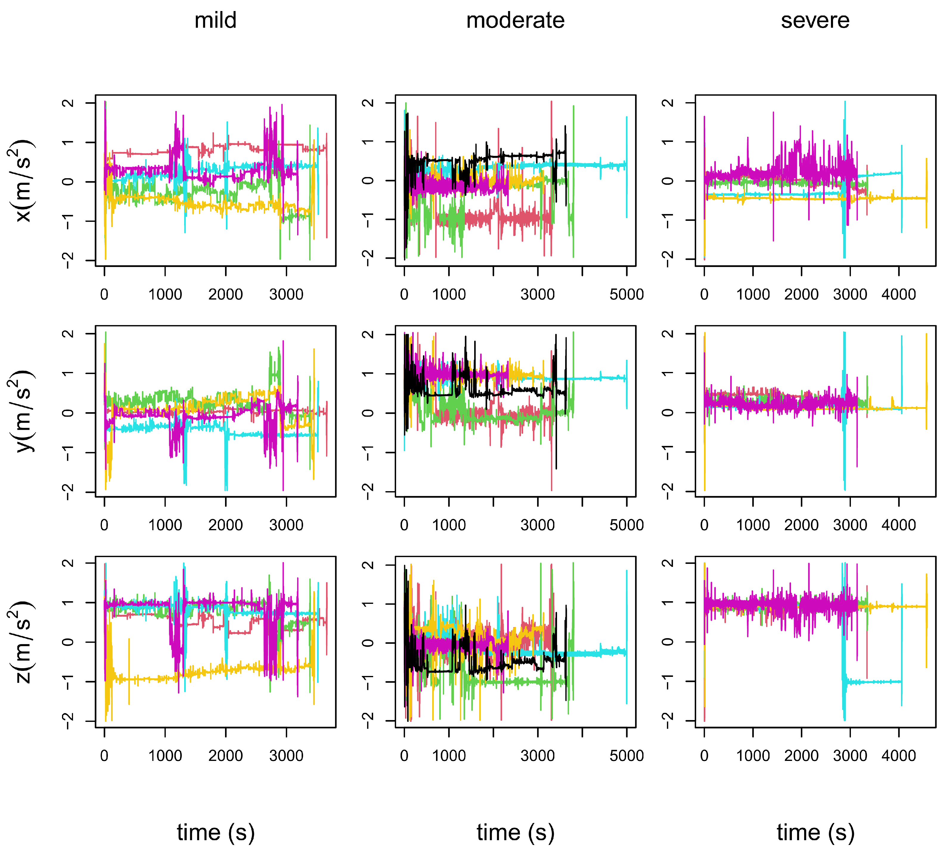
In Figure 4, we exemplify the nature of the dataset by plotting, for three of the patients, the recorded accelerations, in meters per second squared (m/s²), with respect to the time in seconds (s).

• In the left column panels: the five repetitions of patient 19, who is in a mild stage of the disease.
• In the central column panels: the six repetitions of patient 34, who is in a moderate stage of the disease.
• In the right column panels: the five repetitions of patient 35, who is in a severe stage of the disease.

Figure 4. Display of the accelerations (m/s²), in the three coordinate axis (OX: top row, OY: central row and OZ: bottom row) over the time domain (s), of the repetitions of three patients. Each patient is in a different stage of the disease. Left column: mild stage (patient 19). Central column: moderate stage (patient 34). Right column: severe stage (patient 35).

Figure 4. Display of the accelerations (m/s²), in the three coordinate axis (OX: top row, OY: central row and OZ: bottom row) over the time domain (s), of the repetitions of three patients. Each patient is in a different stage of the disease. Left column: mild stage (patient 19). Central column: moderate stage (patient 34). Right column: severe stage (patient 35).

The top row in Figure 4 corresponds to the accelerations with respect to time in the OX coordinate axis, the middle row to the OY coordinate axis and the bottom row to the OZ axis. It is observable from these plots that each repetition is recorded for a different length of time, $L\left(x_{ik}\right)$. Additionally, note that the plots show no apparent difference among the three stages of the disease.

4.5. Results

We find functional $(d,0)$-symmetry when the Sobolev-(2,2) distance is used, in Equation (7) through the use of Equation (8), in the complete sample as well as in the three subsamples corresponding to different severity of dementia (mild, moderate and severe). This is an important finding to get insight into this type of movement data as it tells us information on the symmetry of the underlying distributions. The same results are obtained using the ${\mathbb{L}}_2$ distance due to the functional data points exhibiting little variability over the domain, which is observable from the elements of the dataset displayed in Figure 4.

The corresponding set of centers of $(d,0)$-symmetry can be used to compute the metric depth as outlined in Section 2. Unlike most other functional depth constructions appearing in the literature, the metric depth is known to satisfy the fifth property of the axiomatic definition of statistical functional depth [15]. That property establishes the depth function has to be receptive to the convex hull width across the domain. This is especially relevant here as the elements of functional spaces show a small amount of variation over large parts of the domain. This depth construction automatically accounts for this, giving greater importance to the regions of the domain in which the functional data points exhibit the most variability.

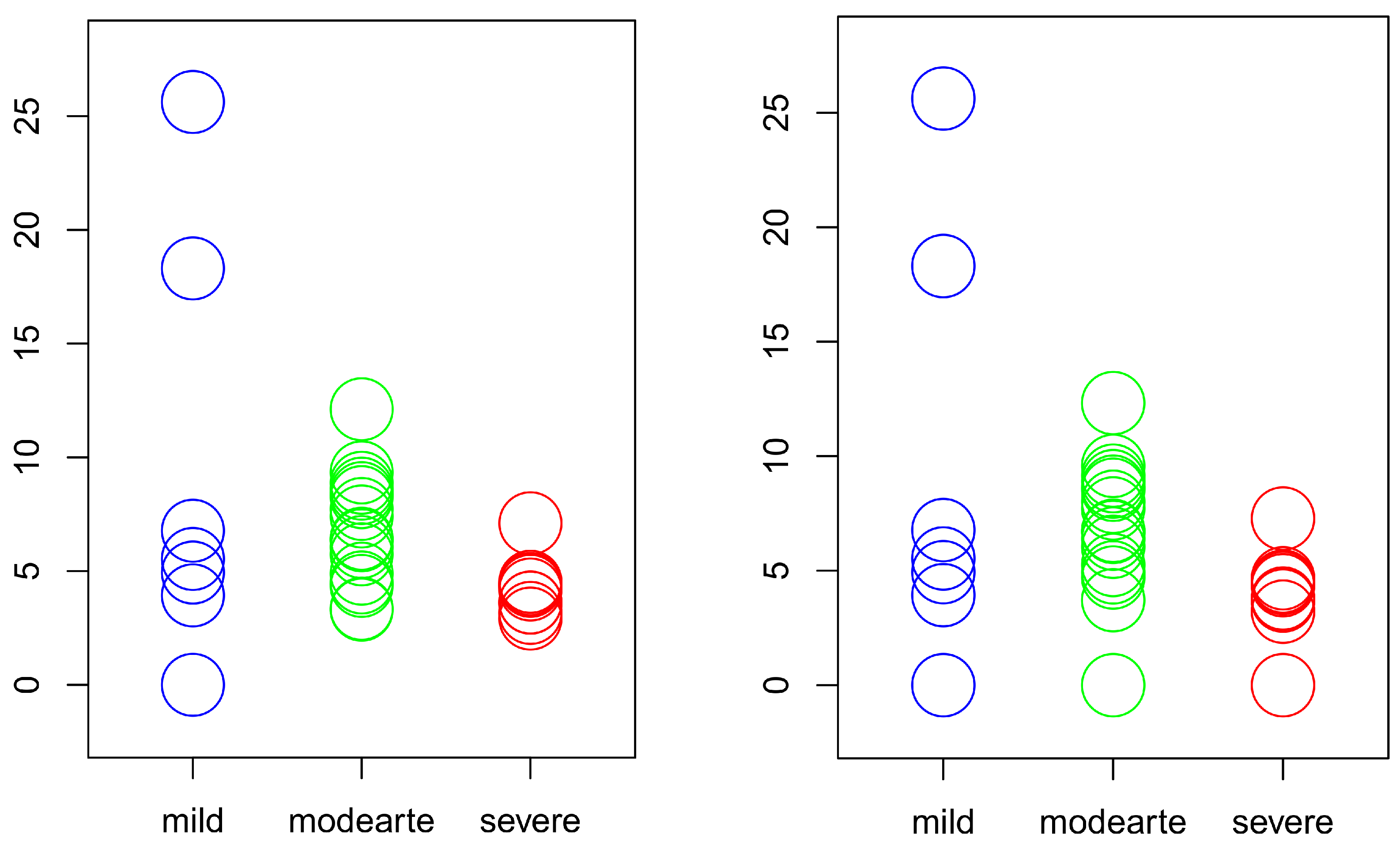
To illustrate the findings, in Figure 5 we display the $I_M$ value of the metric depth, Equation (5), of the elements in each of the three subsets computed with respect to the center of $(d,0)$-symmetry of the complete sample (left plot) and of the three subsamples separately (right plot). As observable from the figure, the center of $(d,0)$-symmetry of the complete sample, which takes $I_M$ value 0, belongs to the subgroup with mild dementia and coincides with the center of symmetry of this subgroup when the center of $(d,0)$-symmetry is computed separately for each of the three subsamples. In fact, the patient corresponding to the center of $(d,0)$-symmetry when computed with respect to the complete sample is the patient labeled as 3 in Table 2. When computing the center of $(d,0)$-symmetry of the patients in the moderate stage of the disease, we obtain that the center of $(d,0)$-symmetry corresponds to the patient labeled as 10. For the severe stage, we obtain the patient labeled as 9.

From the two plots in Figure 5, it can be easily deduced that the variability of the depth values for the mild patients is higher than that for moderate, which likewise is higher than for the severe patients. To check whether this is indeed the case, we perform the permutation tests on the depth commented above in Section 4.2. All the tests are exact permutation tests in this subsection. The p-values resulting from these tests are displayed in Table 4. We have arranged them in two cases:

• The metric depth is computed with respect to the center of $(d,0)$-symmetry of the complete sample. This corresponds to the left plot in Figure 5.
• The metric depth is computed with respect to the center of $(d,0)$-symmetry of each of the three subsamples separately. This corresponds to the right plot in Figure 5.

Table 4. p-values resulting from performing the permutation test on the depth to find distribution, median and deviance from the median differences. The top three rows refer to the tests performed on depth values computed with respect to the complete sample while the bottom three to tests performed on depth values computed for each of the three stages separately. Thus, Complete sample is for using the depth values of the pooled sample and Subsamples for using the depth values computed with respect to each sample separately. The alternative hypothesis for each test is greater than, but for the distribution case that coincides with the not equal alternative. p-values resulting in a rejection at 0.05 significance level are emphasized in bold.

${\mathit{H}}_{\mathit{a}}:$	${\mathfrak{p}}_{\mathit{mild}}>{\mathfrak{p}}_{\mathit{moderate}}$	${\mathfrak{p}}_{\mathit{moderate}}>{\mathfrak{p}}_{\mathit{severe}}$
	Complete Sample
Distribution	0.0202	0.0027
Median	0.8090	0.0158
Deviance	0.0339	0.0030
	Subsamples
Distribution	0.6672	0.0001
Median	0.8242	0.0140
Deviance	0.0320	0.0332

Table 4. p-values resulting from performing the permutation test on the depth to find distribution, median and deviance from the median differences. The top three rows refer to the tests performed on depth values computed with respect to the complete sample while the bottom three to tests performed on depth values computed for each of the three stages separately. Thus, Complete sample is for using the depth values of the pooled sample and Subsamples for using the depth values computed with respect to each sample separately. The alternative hypothesis for each test is greater than, but for the distribution case that coincides with the not equal alternative. p-values resulting in a rejection at 0.05 significance level are emphasized in bold.

${\mathit{H}}_{\mathit{a}}:$	${\mathfrak{p}}_{\mathit{mild}}>{\mathfrak{p}}_{\mathit{moderate}}$	${\mathfrak{p}}_{\mathit{moderate}}>{\mathfrak{p}}_{\mathit{severe}}$
	Complete Sample
Distribution	0.0202	0.0027
Median	0.8090	0.0158
Deviance	0.0339	0.0030
	Subsamples
Distribution	0.6672	0.0001
Median	0.8242	0.0140
Deviance	0.0320	0.0332

For each of the two cases, we have included in the table the p-values resulting of testing whether each two groups of distributions are equal against the alternative in which they differ. The heading of the table is for the greater than alternative instead of not equal so the resulting p-value will coincide, as explained in Section 4.2. Additionally, the table includes a test on which the median on a stage of the disease is less or equal than in the next stage against the alternative in which it is greater and an equivalent test but on the deviation from the median.

The results in Table 4 show a significant difference on the distribution for three out of the four run tests. However, we can say that there is a significant difference in the distribution in the four cases, as the deviance from the median test is able to detect the difference every time. The median test also detects a difference when studying the pair moderate and severe. However, no such difference is detected with the pair mild and moderate. For this case of the median test with the pair mild and moderate, it is worth saying that neither a rejection is obtained for the less than alternative nor for the not equal alternative, although the p-values decrease.

5. Discussion

Many modern datasets consist of functional observations, i.e., data most naturally viewed as realizations of random functions. Typical examples of such data include gene expression levels over time, blood oxygen levels throughout the volume of the brain and, as used for illustration in the present work, accelerations of Alzheimer’s patients when moving freely in a daycare facility. The ease of recording such data make it practically useful, although they present difficulties for its analysis due to their unusual features. Notably:

• There are a different number of recordings for each patient.
• Each recording is over a different time domain.
• Each recording is observed over a different grid.

Our functional data analysis based on new notions of functional symmetry and depth introduced in [11] applies without complications in this setting. This notion of functional symmetry has the advantage of being truly conceived for functional data and it adapts to the characteristics of the data, through the metric. Thus, it is not an extension of a multivariate notion like the others existing in the literature. The instance of depth used, the metric depth, does have two advantages over the others in the literature:

• The involved center of symmetry is a truly functional center of symmetry.
• It is the only existing instance of depth that satisfies the notion of statistical functional depth.

Most existing data of this type are recorded in a controlled environment such as a laboratory and not just by the use of a smartphone in a quite free environment. This dataset, however, has been previously used in [3,4] with the aim of performing supervised classification. There, black-box techniques were applied and so the objective in this paper has been to understand the characteristic(s) that differentiate among the distributions of the stages of Alzheimer’s disease. The proposed methodology is able to distinguish between patients at different stages of the disease based on the accelerometer data. In particular, we found that the distribution of acceleration differs between each stage of the disease. We observe that those differences are mainly due to scale differences. As for ensuring the validity of the methodology used, in addition to the broad results covered in [11], we have provided a simulation study to emulate the analysis performed on the real data when the ground truth is known. Analogous to the performed analysis based on the recorded accelerations, future research could include an analysis on the velocities.

References

- Mayeux, R.; Sano, M. Treatment of Alzheimer’s disease. N. Engl. J. Med. 1999, 341, 1670–1679. [Google Scholar] [CrossRef]
- Reisberg, B.; Ferris, S.H.; de Leon, M.J.; Crook, T. The Global Deterioration Scale for assessment of primary degenerative dementia. Am. J. Psychiatry 1982, 139, 1136–1139. [Google Scholar] [PubMed] [Green Version]
- Bringas, S.; Salomón, S.; Duque, R.; Lage, C.; Montaña, J.L. Alzheimer’s Disease stage identification using deep learning models. J. Biomed. Inform. 2020, 109, 103514. [Google Scholar] [CrossRef] [PubMed]
- Nieto-Reyes, A.; Duque, R.; Montaña, J.L.; Lage, C. Classification of Alzheimer’s patients through ubiquitous computing. Sensors 2017, 17, 1679. [Google Scholar] [CrossRef] [PubMed] [Green Version]
- Park, S.Y.; Staicu, A.M. Longitudinal functional data analysis. STAT Int. Stat. Inst. 2015, 4, 212–226. [Google Scholar] [CrossRef] [Green Version]
- Ferraty, F.; Vieu, P. Nonparametric Functional Data Analysis; Springer Series in Statistics; Springer: New York, NY, USA, 2006. [Google Scholar]
- Ramsay, J.O.; Silverman, B.W. Functional Data Analysis; Springer Series in Statistics; Springer: New York, NY, USA, 2005. [Google Scholar]
- Zuo, Y.; Serfling, R. On the performance of some robust nonparametric location measures relative to a general notion of multivariate symmetry. J. Statist. Plann. Inference 2000, 84, 55–79. [Google Scholar] [CrossRef]
- Zuo, Y.; Serfling, R. General notions of statistical depth function. Ann. Statist. 2000, 28, 461–482. [Google Scholar] [CrossRef]
- Kallenberg, O. Probabilistic Symmetries and Invariance Principles; Probability and Its Applications; Springer: New York, NY, USA, 2005. [Google Scholar]
- Nieto-Reyes, A.; Battey, H. A topologically valid construction of depth for functional data. J. Multivar. Anal. 2021, 184, 104738. [Google Scholar] [CrossRef]
- Fukunaga, K.; Koontz, W.L.G. Application of the Karhunen-Loève Expansion to Feature Selection and Ordering. IEEE Trans. Comput. 1970, 19, 311–318. [Google Scholar] [CrossRef] [Green Version]
- Dudley, R.M. Uniform Central Limit Theorems; Cambridge Studies in Advanced Mathematics, Series Number 63; Cambridge University Press: Cambridge, UK, 1999. [Google Scholar]
- Hall, P. Two-sided bounds on the rate of convergence to a stable law. Zeitschrift für Wahrscheinlichkeitstheorie und Verwandte Gebiete 1981, 57, 349–364. [Google Scholar] [CrossRef]
- Nieto-Reyes, A.; Battey, H. A topologically valid definition of depth for functional data. Stat. Sci. 2016, 31, 61–79. [Google Scholar] [CrossRef]
- Chakraborty, A.; Chaudhuri, P. On data depth in infinite dimensional spaces. Ann. Inst. Stat. 2014, 66, 303–324. [Google Scholar] [CrossRef] [Green Version]
- Dutta, S.; Ghosh, A.-K.; Chaudhuri, P. Some intriguing properties of Tukey’s halfspace depth. Bernoulli 2011, 17, 1420–1434. [Google Scholar] [CrossRef] [Green Version]
- Tukey, J. Mathematics and the picturing of data. In Proceedings of the International Congress of Mathematicians, Vancouver, BC, Canada, 21–29 August 1974; Canadian Mathematical Congress: Montreal, QC, Canada, 1975; pp. 523–531. [Google Scholar]
- Liu, R.Y. On a notion of data depth based on random simplices. Ann. Statist. 1990, 18, 405–414. [Google Scholar] [CrossRef]
- López-Pintado, S.; Romo, J. On the concept of depth for functional data. J. Amer. Statist. Assoc. 2009, 104, 718–734. [Google Scholar] [CrossRef] [Green Version]
- López-Pintado, S.; Romo, J. A half-region depth for functional data. Comput. Statist. Data Anal. 2011, 55, 1679–1695. [Google Scholar] [CrossRef] [Green Version]
- Cuevas, A.; Febrero, M.; Fraiman, R. Robust estimation and classification for functional data via projection-based depth notions. Comput. Statist. 2007, 22, 481–496. [Google Scholar] [CrossRef]
- Cuesta-Albertos, J.A.; Nieto-Reyes, A. The random Tukey depth. Comput. Statist. Data Anal. 2008, 52, 4979–4988. [Google Scholar] [CrossRef]
- Cuesta-Albertos, J.A.; Nieto-Reyes, A. Functional Classification and the Random Tukey Depth: Practical Issues. In Combining Soft Computing and Statistical Methods in Data Analysis; Borgelt, C., González-Rodríguez, G., Trutschnig, W., Lubiano, M.A., Gil, M.Á., Grzegorzewski, P., Hryniewicz, O., Eds.; Springer: Berlin/Heidelberg, Germany, 2010; pp. 123–130. [Google Scholar]
- Chakraborty, A.; Chaudhuri, P. The spatial distribution in infinite dimensional spaces and related quantiles and depths. Ann. Statist. 2014, 42, 1203–1231. [Google Scholar] [CrossRef] [Green Version]
- Richter, S.J.; McCann, M.H. Permutation tests of scale using deviances. Commun. Stat. Simul. Comput. 2017, 46, 5553–5565. [Google Scholar] [CrossRef] [Green Version]
- Higgins, J.J. An Introduction to Modern Nonparametric Statistics; Brooks/Cole: Pacific Grove, CA, USA, 2003. [Google Scholar]
- Kolmogorov, A. Sulla determinazione empirica di una legge di distribuzione. Giorn. Ist. Ital. Attuar. 1933, 4, 83–91. [Google Scholar]
- Smirnov, N. Table for estimating the goodness of fit of empirical distributions. Ann. Math. Stat. 1948, 19, 279–281. [Google Scholar] [CrossRef]
- Ijmker, T.; Lamoth, C.J.C. Gait and cognition: The relationship between gait stability and variability with executive function in persons with and without dementia. Gait Posture 2012, 35, 126–130. [Google Scholar] [CrossRef]
- Kirste, T.; Hoffmeyer, A.; Koldrack, P.; Bauer, A.; Schubert, S.; Schroeder, S.; Teipel, S. Detecting the effect of Alzheimer’s disease on everyday motion behavior. J. Alzheimer’s Dis. 2014, 38, 121–132. [Google Scholar] [CrossRef] [PubMed]
Figure 1.
Top panels: sample draws from a standard bivariate normal distribution (left) and a dataset of raw univariate functional data (right). Bottom panel: sample draws from a standard normal distribution in dimension one. The color of the elements in each of the three plots represent the depth based on the distance to the center of symmetry of the sample.
Figure 2.
Observations from a mixture of Gaussian processes on [0, 1]. Mixture components are mean zero and have covariance structure where with probability with probability and with probability Realizations corresponding to each mixture component are highlighted in the respective panels from left () to right ().
Figure 3.
Symmetries induced in the domain of the integration of a Gaussian process with correlation length 1 minus its center of symmetry versus the integral of its first derivative (left) and of the first derivative versus the second (right). The color represents the metric depth in Sobolev-(2,2) distance (left) and in the Sobolev-(2,2) distance minus the distance (right), with the center depicted by a white dot.
Figure 5.
Representation of the depth value for the 35 Alzheimer’s patients computed with respect to the center of symmetry of the complete sample (left plot) and of the three subsamples separately (right plot).