A New Ensemble Method for Detecting Anomalies in Gene Expression Matrices

Abstract

One of the main problems in the analysis of real data is often related to the presence of anomalies. Namely, anomalous cases can both spoil the resulting analysis and contain valuable information at the same time. In both cases, the ability to detect these occurrences is very important. In the biomedical field, a correct identification of outliers could allow the development of new biological hypotheses that are not considered when looking at experimental biological data. In this work, we address the problem of detecting outliers in gene expression data, focusing on microarray analysis. We propose an ensemble approach for detecting anomalies in gene expression matrices based on the use of Hierarchical Clustering and Robust Principal Component Analysis, which allows us to derive a novel pseudo-mathematical classification of anomalies.

1. Introduction

Real datasets often contain observations that behave differently from the majority of the data. If an occurrence differs from the dominant part of the data, or if it is sufficiently unlikely under the assumed data probability model, it is considered an anomaly or outlier.

Outliers may be caused by errors, but they may also result from exceptional circumstances or belong to a different population of data. On the one hand, anomalies may adversely affect the conclusions drawn from data analysis; on the other hand, they may contain important information. Thus, outlier detection is about the interest in the outliers themselves or the fact that they may contaminate the subsequent statistical analysis. In statistics, an outlier is an observation that falls outside the overall pattern of a distribution [1]. However, it is difficult to determine how much a value must deviate to be called an outlier. Robust statistics are designed to detect outliers by first fitting the majority of the data and then flagging data points that deviate [2]. In the biomedical field, the correct identification of outliers is of great importance: depending on the type of analysis to be performed, biologists can decide whether or not these data should be removed.

In this work, we address the problem of detecting outliers in Gene Expression Profiling (GEP) data, focusing on microarray data containing gene expression values for a given number of samples labeled with a biological class (tumor type or experimental condition). In this type of data, there are generally two main types of outliers, which refer to the case where the instances are genes or samples, respectively [3]. The former is present when a gene has abnormal expression values in one or more samples from the same class, whereas the latter can be dually seen as samples that belong to a different class present in the data (often referred to as mislabeled samples) or as samples that do not belong to any class present in the data (called abnormal samples or outliers).

The origin of these outliers may be ambiguous; they may result from an undiscovered biological class, poor class definitions, experimental error, or extreme biological variability. Note that, when we say that an anomalous sample does not belong to its class, we are not necessarily disputing the validity of its designation. Indeed, a sample may still be a tumor, but at the same time it could have expression levels that are significantly different from those of other tumor samples. Using learning models to analyze data affected by outliers may even lead to incorrect conclusions. In the past, the impact of outliers was rarely considered when analyzing data from standard microarrays. According to the new current, outlier detection is used as preprocessing for data cleaning. However, it is essential to emphasize that, in many cases, outliers may simply be the result of natural variability in the data.

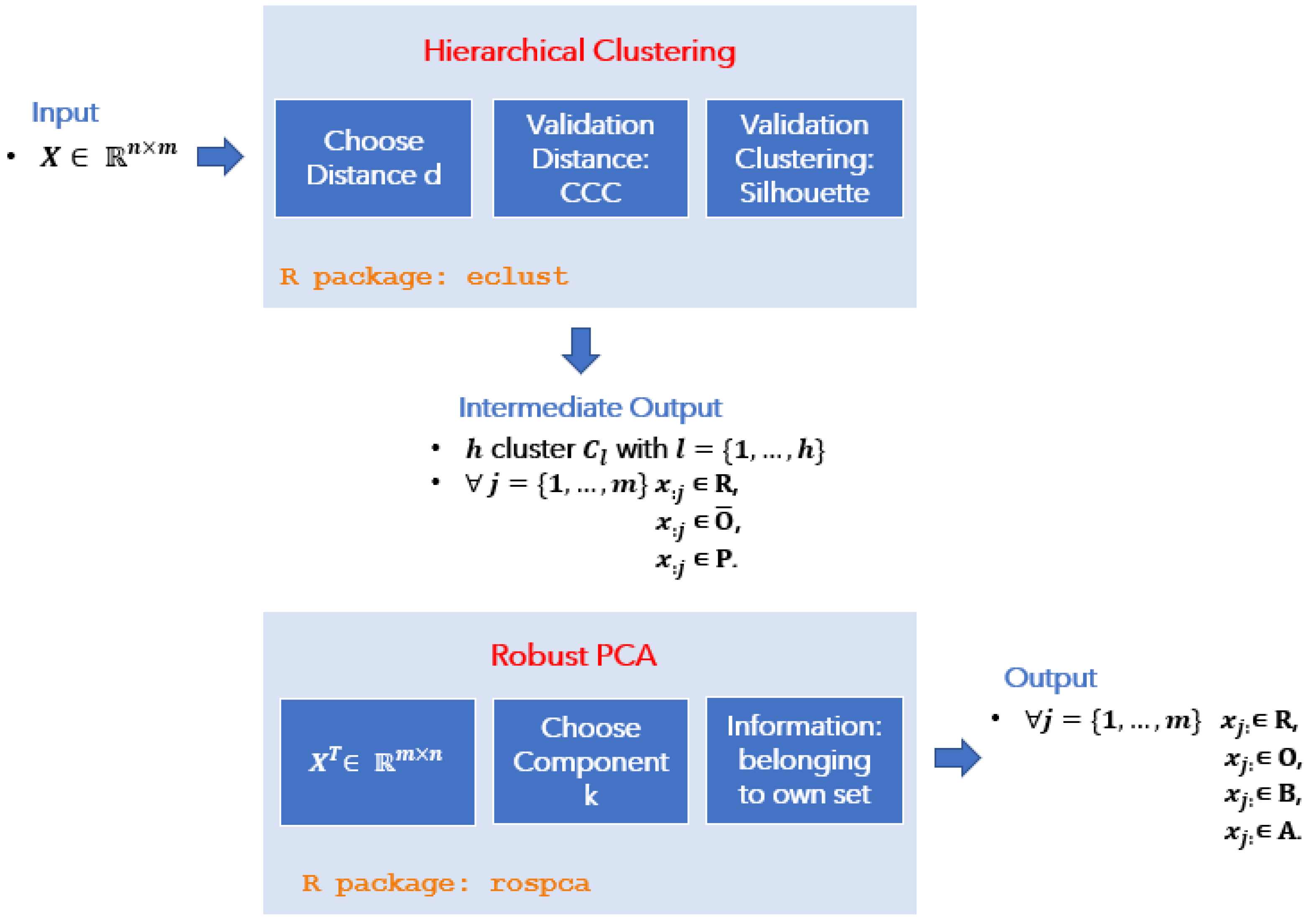
In this paper, we propose a novel ensemble approach that combines Hierarchical Clustering and Robust Principal Component Analysis to detect outliers in GEP data (these two techniques are generally not used for this purpose in this context), with an additional decision-making model (the anomaly detection tool) that can provide a pseudo-mathematical classification of outliers based on their biological nature.

The paper is organized as follows. Section 2 gives a brief overview of anomaly detection algorithms, also focusing on the microarray context, while Section 3 illustrates the proposed ensemble mechanism. Section 4 describes the experimental results obtained when applying the proposed methodology to six different datasets (two artificial and four real medical databases), discussing also some biological aspects and considerations. In Section 5, comparisons with the most commonly used anomaly detection techniques are reported with some discussions on the advantages of the proposed approach. Finally, conclusions and directions for future research are outlined in Section 6.

2. Methods for Outliers Detection

Detecting anomalies in real-world data is a difficult problem that can be addressed using a variety of mathematical techniques, ranging from standard univariate strategies to more comprehensive multivariate analysis. A comprehensive and complete review of the most commonly used methods can be found in References [4,5]. In the context of a multivariate approach, clustering and Low-Rank reduction mechanisms proved to be the most important. Clustering is an unsupervised learning mechanism capable of finding structures and similar patterns in collections of unlabeled data [6]. A cluster refers to a group of objects that are “similar” to each other (with respect to some measure) and “dissimilar” to objects belonging to other clusters.

Thus, the outliers are those samples that belong to a separate micro-cluster because they are far away from most of the other data. They are usually identified by increasing the number of clusters and for this reason it is necessary to define a measure of dissimilarity between clusters. In the analysis of gene expression data, the correlation-based measure (i.e., the one based on Pearson Correlation Coefficient) is considered the most appropriate dissimilarity measure when clusters of observations with the same overall profiles are obtained. Correlation works well for gene expression in clustering of samples and genes, although Pearson’s correlation is quite sensitive to outliers. In samples clustering, this issue is irrelevant because the correlation is among thousands of genes, whereas when genes have to be clustered, it is important to be aware of the possible impact of outliers. Assigning weight values to samples [7] is a possible way to improve the performance of the Pearson distance in handling outliers. On the other hand, distance is not the only choice to be made in clustering algorithms; the appropriate mechanism that defines how to separate two different clusters is also a task to be addressed. To tune these hyperparameters, either the Cophenetic Correlation Coefficient (CCC) and the Silhouette coefficient [8] could be adopted. The CCC expresses the correlation between the original dissimilarity matrix and the one derived based on the classification. Usually, a $CCC\ge 0.8$ means a good match, while $CCC<0.8$ indicates that the dendrogram is not a good representation of the relationships between the objects.

We give below the definition of the Silhouette coefficient, used to validate the quality of the clustering. Based on the clustering vector and the set of distances, the algorithm computes the dissimilarity of a point $x_i$ to its current class and the lowest dissimilarity of the point to other classes, through $a\left(x_i\right)$ and $b\left(x_i\right)$, respectively, defined as follows, for all $x_i\in C_i$:

$$a\left(x_i\right)=\frac{1}{|C_i|-1}\sum _{j\in C_i,i\ne j}d(x_i,x_j),\mathrm{and}$$

(1)

$$b\left(x_i\right)=\underset{k\ne i}{min}\frac{1}{|C_k|}\sum _{j\in C_k}d(x_i,x_j).$$

(2)

Then, the Silhouette coefficient is set to zero when $|C_i|=1$ by definition and usually ranges in $[-1,1]$, in the other cases it can be defined as

$$s\left(x_i\right)=\frac{b\left(x_i\right)-a\left(x_i\right)}{max\{a\left(x_i\right),b\left(x_i\right)\}}.$$

(3)

Its maximum value 1 indicates a better match with the current cluster, while $-1$ means that the point actually belongs to the other class or a so-called “neighboring cluster”.

Table 1. Structures corresponding to particular Silhouette coefficient ranges.

SC	Interpretation
0.71–1.0	A strong structure was found.
0.51–0.70	A reasonable structure was found.
0.26–0.50	The structure is weak and may be artificial.
<0.25	No substantial structures have been found.

shows the range values of the Silhouette coefficients associated with the corresponding structures and usually adopted in literature panorama [9].

Among Low Rank reduction mechanisms, Robust Principal Component Analysis (ROBPCA) has been widely used in GEP data analysis to identify subgroups with specific biological characteristics that correlate with different clinical behaviors [10,11,12]. It combines the strengths of Projection-Pursuit techniques (PP) [13] and robust covariance estimation. The former is used to reduce initial dimensionality, while the latter, particularly the Minimum Covariance Determinant (MCD) estimator, is used to obtain a smaller data space. To our knowledge, however, this is the first time that ROBPCA has been applied to outlier detection in microarray data, although it has recently been used for the analysis of RNA-seq data, which requires a more complex sample preparation protocol and analysis compared to microarray data [14].

Formally, consider a data matrix ${\mathbf{X}}_{n,p}\in {\mathbb{R}}^{n\times p}$, where n indicates the number of the observations, and p the original number of variables, and the ROBPCA method proceeds in three main steps:

• the data is preprocessed so that the transformed data lies in a subspace whose dimension is at most $n-1$;
• a preliminary covariance matrix $S_0$ is constructed and used to select the number of components k that are subsequently retained, resulting in a k-dimensional subspace that is well fitted to the data;
• data points are projected onto this subspace, where their location and scatter matrix are robustly estimated, from which their k non-zero eigenvalues ${\ell }_1,\dots {\ell }_k$ are computed. The corresponding eigenvectors are the k robust principal components.

Let $P_{p,k}$ be the $p\times k$ eigenvector matrix (with orthogonal column vectors); the location estimate is denoted by the p-variate column vector $\widehat{\nu }$ and called the robust center. The scores are the entries of the $n\times k$ matrix

$$T_{n,k}=(X_{n,p}-1_n{\widehat{\nu }}^{\top })·P_{p,k}.$$

(4)

The k robust principal components generate a $p\times p$ robust scatter matrix S of rank k given by

$$S=P_{p,k}{L}_{k,k}{P}_{p,k}^{\top },$$

(5)

where $L_{k,k}$ is the diagonal matrix with the eigenvalues ${\ell }_1,\dots {\ell }_k$.

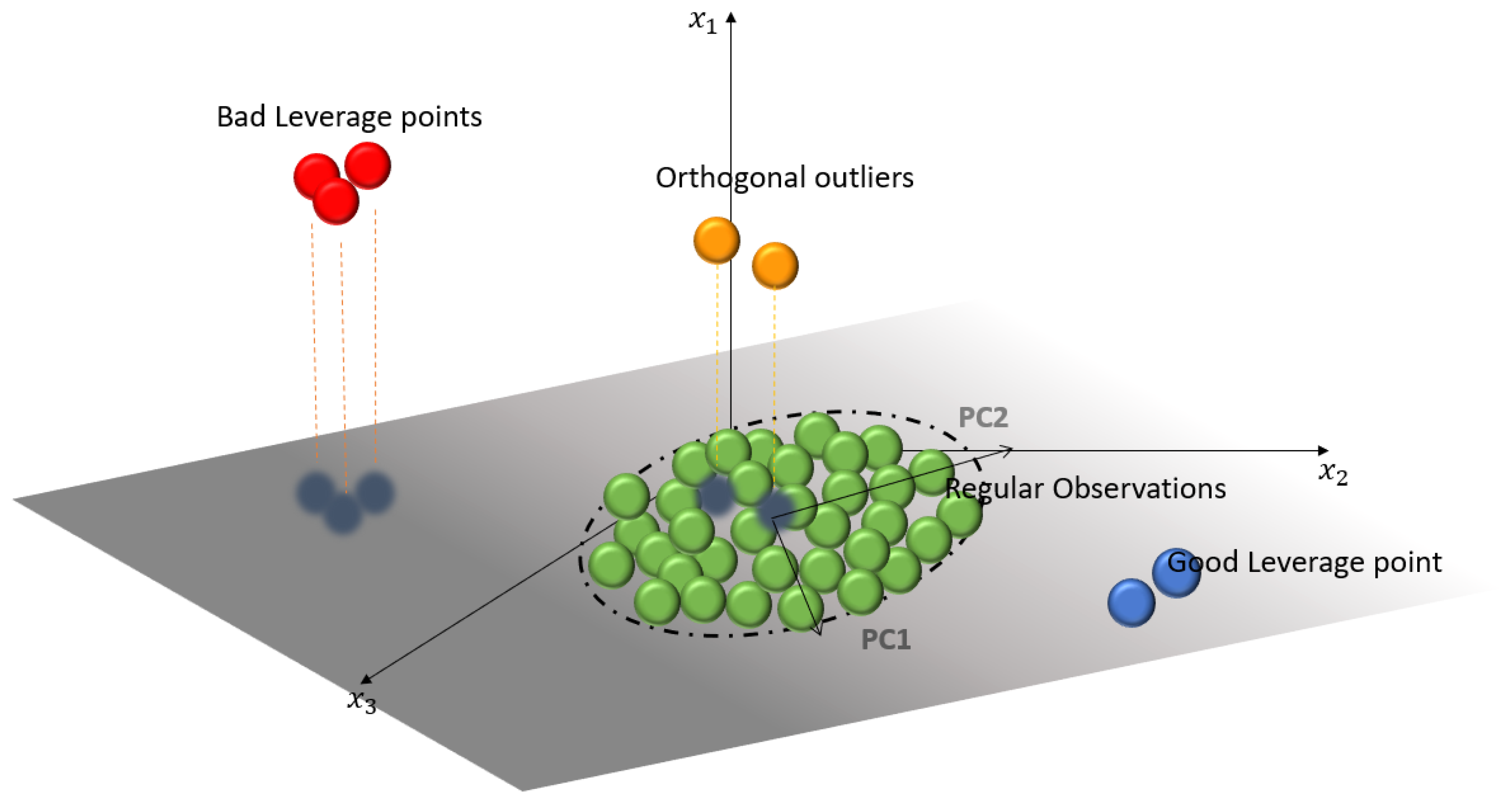
Similar to classical PCA, the ROBPCA method is locationally and orthogonally equivariant, properties that are non-trivial for other robust PCA estimators [2,15]. It should be emphasised that one of the advantages of using PCA-related mechanisms is a feasible outlier classification that takes into account the positions of outliers with respect to the projected subspace and also provides a useful interpretation of these positions.

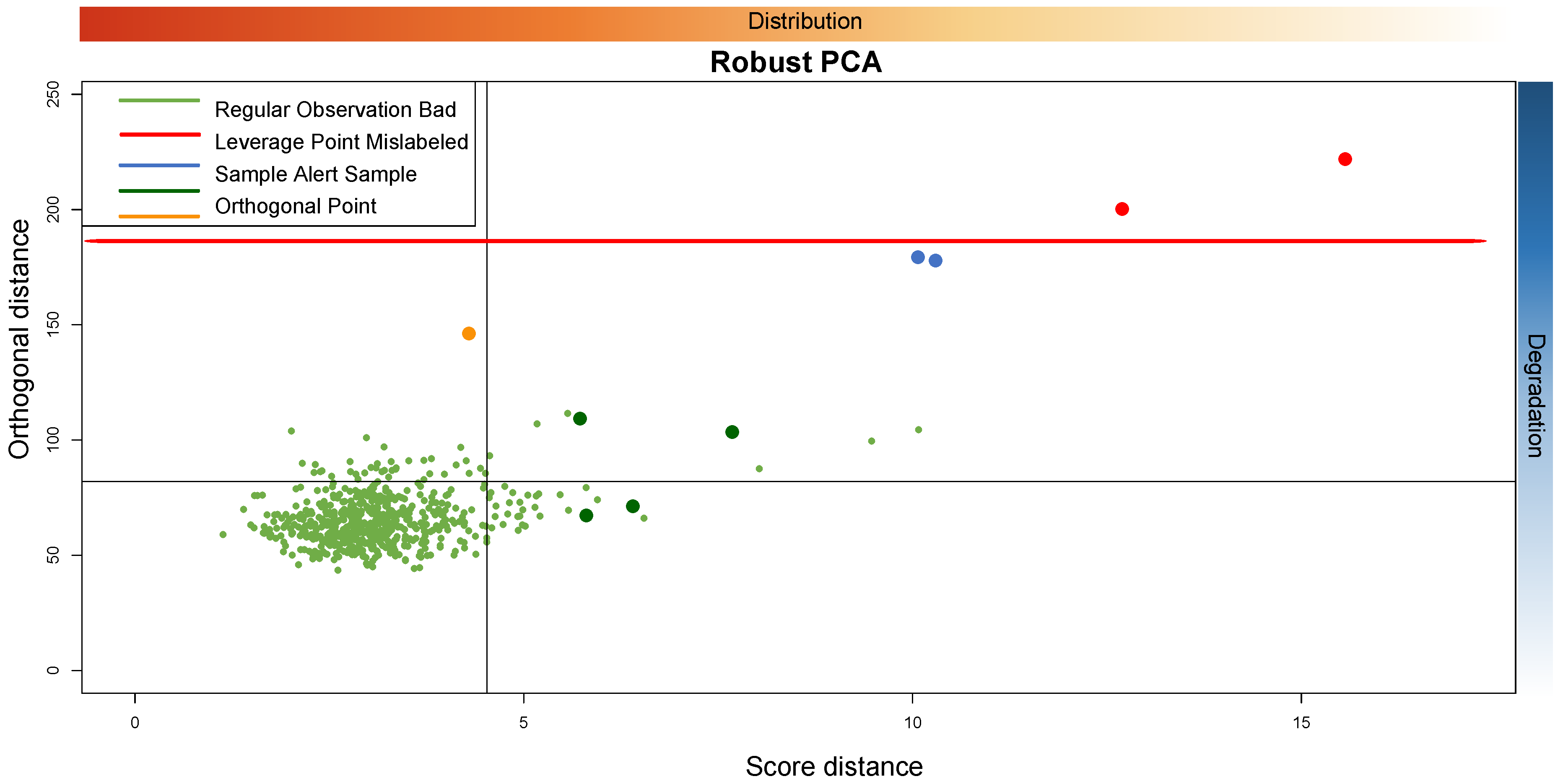
An example of this behavior is shown in Figure 1, where four types of points can be distinguished, depending on the location of the observation. These points can be categorized as: Regular Observations (ROs), which form a homogeneous group near the PC subspace generated by the principal components; Good Leverage Points (GLPs), which are at the same plane as the PC subspace but distant from the ROs; Orthogonal Observations (OOs), which have a large orthogonal distance to the PC subspace, but whose projection is on the PC subspace; and, finally, Bad Leverage Points (BLPs), which have a large orthogonal distance such that the projection on the PC subspace is away from ROs.

To understand and quantify how far an observation is from the center of the ellipse, defined by ROs (score $=0$ was chosen as reference), two distances can be used: the Score Distance, $S{D}_i$, and the Orthogonal Distances, $O{D}_i$, defined as follows:

$$S{D}_i=\sqrt{\sum _{j=1}^k\frac{t_{ij}^2}{{\ell }_j}},\mathrm{for}i=1,\dots ,n,$$

(6)

with ℓ the eigenvalues of the dispersion matrix MCD, and $t_{ij}$ the robust scores for each $j=1,\dots ,k$, is a measure of the distance between an observation belonging to the PC k-dimensional subspace and the origin of this subspace; and

$$O{D}_i=\parallel x_i-\widehat{\mu }-P_{p,k}{t}_i^{\top }\parallel ,\mathrm{for}i=1,\dots ,n,$$

(7)

where each $t_i^{\top }$ is the i-th row of $T_{n,k}$, and $\widehat{\mu }$ is the robust estimate of the center, which measures the deviation (i.e., lack of fit) of an observation from the PC k-dimensional subspace.

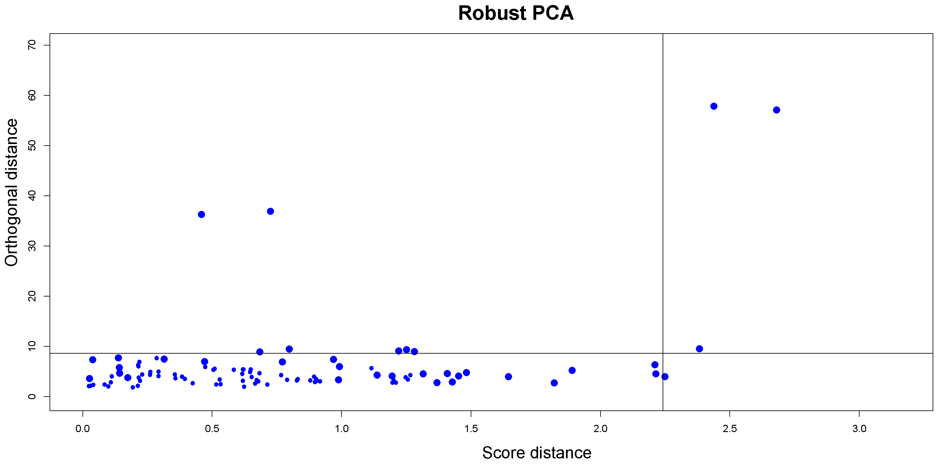
Based on these measures, the diagnostic plot (DD-plot or outlier map) can be plotted with $S{D}_i$ on the horizontal axis and $O{D}_i$ on the vertical axis to distinguish between ROs and the three types of outliers. To classify all observations, two cutoff lines are drawn according to the data. Since it is known that the distance adopted to construct the tolerance ellipsoid (the squared Mahalnobis distances for normally distributed scores) follows a $\chi$-squared distribution approximately, the cutoff value of the horizontal axis is obtained from the $0.975$ quantile of this distribution with k degrees of freedom:

$${\mathrm{cutoff}}_{SD}=\sqrt{{\chi }_{k,0.975}^2}.$$

(8)

On the other hand, even if the distribution of the $O{D}_i$ for the generic i, it is not known exactly, literature results allow to approximate them by a normal distribution with particular mean and variance estimated using the MCD [10]. Defining in this way the cutoff for the vertical axis as:

$${\mathrm{cutoff}}_{OD}={(\widehat{\mu }+\widehat{\sigma }{z}_{0.975})}^{\frac{3}{2}},$$

(9)

where $\widehat{\mu }$ and $\widehat{\sigma }$ are the MCD estimates for the mean and standard deviation of the above normal distribution, and $z_{0.975}$ is the $97.5\%$ quantile of the Gaussian distribution. Figure 2 illustrates an example of the outlier map described.

As with standard PCA approaches, their robust variants require a criterion for selecting the number of principal components. We adopt the mechanism proposed in Reference [10], which selects k components according to the following empirical Rayleigh rule:

$$\frac{{\displaystyle \sum _{j=1}^k}{\ell }_j}{{\displaystyle \sum _{j=1}^r}{\ell }_j}\approx 90\%,$$

(10)

where ${\ell }_j$ for $j=1,\dots ,k$ are the eigenvalues of $S_0$, the robust covariance matrix of the data and r the rank of $S_0$. However, there are some other criteria proposed in literature for selecting k, ranging from the use of the formula $\frac{{\ell }_k}{{\ell }_1}\ge {10}^{-3}$ to the use of more complex information based criteria and cross-validation approaches [16,17,18].

In the context of gene expression array analysis, state-of-the-art standard methods for detecting anomalies in microarrays, which are considered reference methods, are implemented in the Bioconductor package arrayQuality [19,20]. These perform univariate analysis based on two independent methods that assign a rank to each sample. The first technique takes one sample at time and compares its probability distribution to that of the entire dataset using a Kolmogorov-Smirnov statistic, assuming the intrinsic similarity measure is that based on the statistical distribution. Instead, the other technique simply ranks each sample according to that sample’s total information across all genes (by summing over expression levels). In both approaches, the outlier sample is selected at the end by performing the standard univariate detection method according to the rank score.

3. Proposed Approach

To detect anomalous samples in microarray datasets and provide a possible feasible outlier classification, we combined Hierarchical Clustering (HC) and Robust PCA performing them sequentially. The ensemble approach obtained uses the first technique to derive a preliminary view of the dataset, where the choice of the distance is determined by the CCC and the clustering is validated by the Silhouette coefficient. The second technique for characterizing the nature of the outlier is based on the position of the sample on the DD-plot. The workflow of the proposed approach detailed with the packages used to perform each block is depicted in Figure 3.

The proposed framework identifies different categories of samples based on the fitting of the data by the two techniques performed sequentially and on the classification in the Section 2, that labels data samples as ROs, GLPs, BLPs, and OOs. In addition, an Alert Sample-type (AS) is included: this is identified as an observation with a lower silhouette (below a pre-selected threshold) and they should not indicate strictly anomalous samples, but samples not properly fitting the data. The Algorithm 1 describes the identification procedure that encodes the sample classification mentioned above.

Algorithm 1: Alert Samples identifier

4. Experimentation

This section is devoted to evaluating the performance of the proposed methodology on both artificial and real biological datasets. All numerical results were obtained testing the proposed approach in the R environment [21] run on a 16Gb RAM, I7 octa core machine.

Concerning the HC, as discussed in Section 2, we have used this general framework with the Pearson distance, while the CCC was adopted to select the most appropriate method. On the other hand, referring to the approach Low-Rank, the number of PCs was selected according to the empirical criterion in (10).

4.1. Synthetical Datasets

Two artificial datasets were constructed to investigate different key aspects of this study. The first dataset aims to simulate the typical structure of the cancer dataset [22,23,24] to estimate the biological aspects of the chosen techniques. The second artificial dataset was designed instead to investigate, from a mathematical point of view, the nature of the outliers and to try to mimic what happens in a biological context.

As a first step for our study, we simulated a typical cancer dataset with known outliers as proposed in Reference [24]. Each dataset contains two clearly distinguishable sample classes. The abnormal samples do not belong to either class or are simply mislabeled.

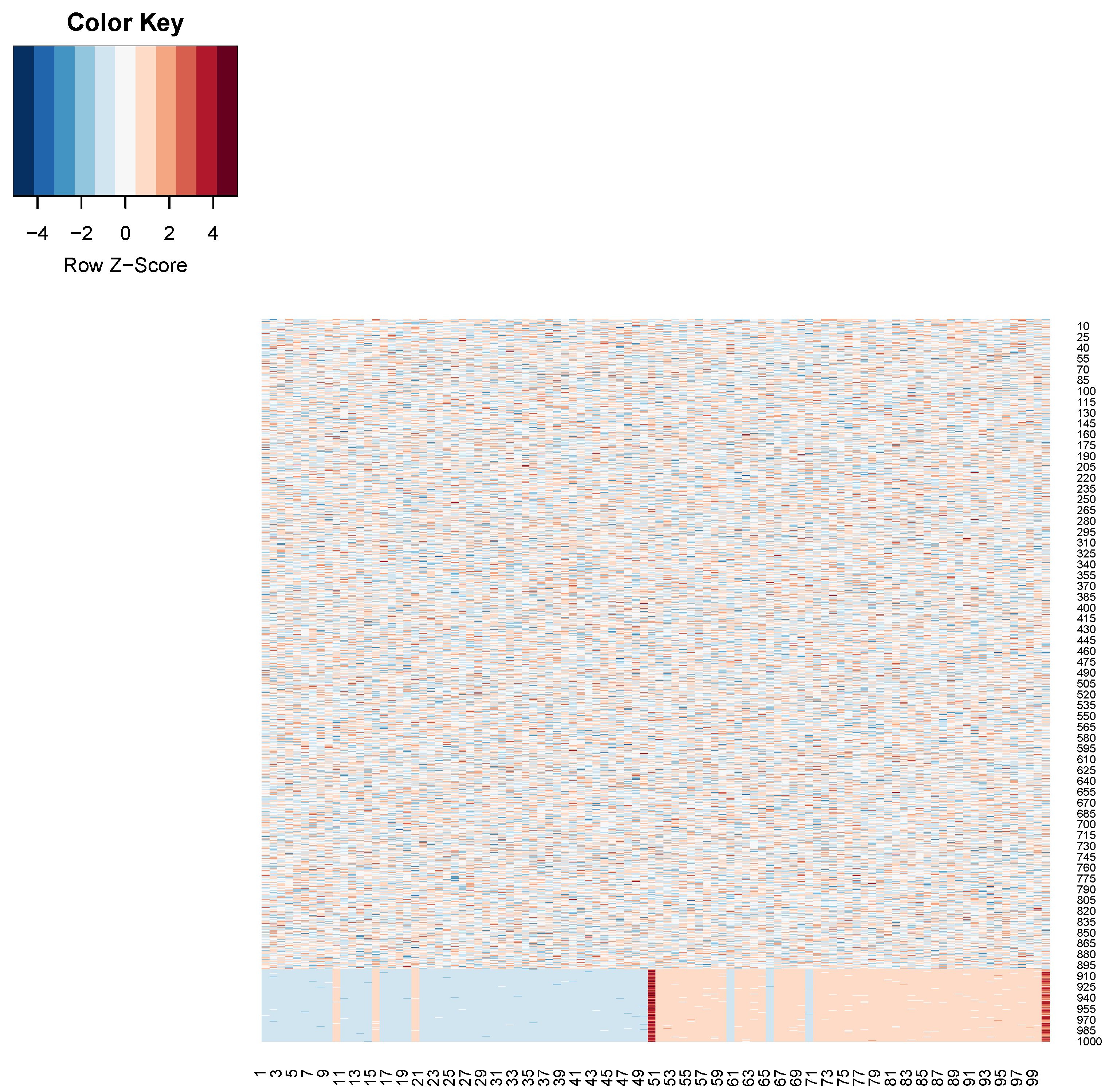
We have 1000 genes in the rows and 100 samples in the columns (50 for each class). The first 900 rows are drawn from the same normal distribution for both classes, and the remaining 100 were drawn from different distributions for samples of classes $C_1$ and $C_2$, respectively. In addition, three samples of class $C_1$ were swapped with three samples of the second class $C_2$. Finally, the last sample of each class was replaced by one with a different distribution (e.g., the Poisson distributions with ${\lambda }_1=30$ and ${\lambda }_2=35$, respectively). A graphical representation of this structure can be found in Figure 4.

Table 2. Cophenetic Correlation Coefficient (CCC) corresponding to the various methods.

Linkage Method	Average	Ward.D2	Complete	Single	Centroid
CCC	$0.92$	$0.35$	$0.58$	$0.9$	$0.64$

and Figure 5 give the CCC value and the Silhouette index, respectively, which are used to validate the quality of the clustering. In particular, in Table 2, the CCC values for different methods allow the selection of the average linkage as the best method for this clustering. The clustering associated with the highest CCC value was then validated by the Silhouette coefficient, which is equal to 0.35. As can be seen in Figure 5, the two techniques give the same results, in particular HC positions the mislabeled outliers in the right class, while the abnormal type outliers form a separate cluster.

Subsequently, the ROBPCA method detects more qualitative information, as described in Section 2. In this case, the “mislabeled” samples are labeled as GLPs, as shown in Figure 6.

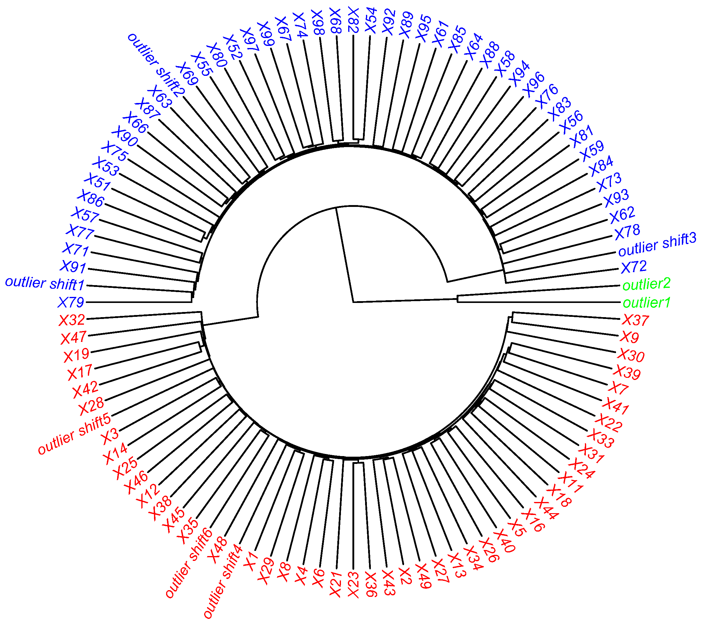
A second artificial dataset was created to check whether outliers detected by the proposed ensemble methodology can be endowed with some statistical properties.

From a statistical point of view, an outlier is seen as an observation that lies outside the overall pattern of a distribution, so the dataset was constructed so that most samples satisfy a normal distribution, with only a few anomalous samples generated with probability distributions that do not verify the Central Limit Theorem (CLT). Specifically, the data matrix $X_{n,m}$, with $n=1000$ and $m=300$, $s=m-4$ has normal $X_{:j}\sim \mathcal{N}(0,1)$ (for $j=1,\dots ,s$) samples and only four anomalies.

We reproduce a bimodal trend of the sampling distributions by setting 100 rows in $X_{n,m}$ to a normal distribution $\mathcal{N}(3,0.5)$. As for the four outliers, two of them retain the normal distribution, with different mean and variance (1 and $1.1$ for the means and 1 and $0.9$ for the values of the second pulse); while the remaining two are generated without central t-students with 2 and $2.1$ degrees of freedom and 2 and $2.2$ without central parameter, respectively.

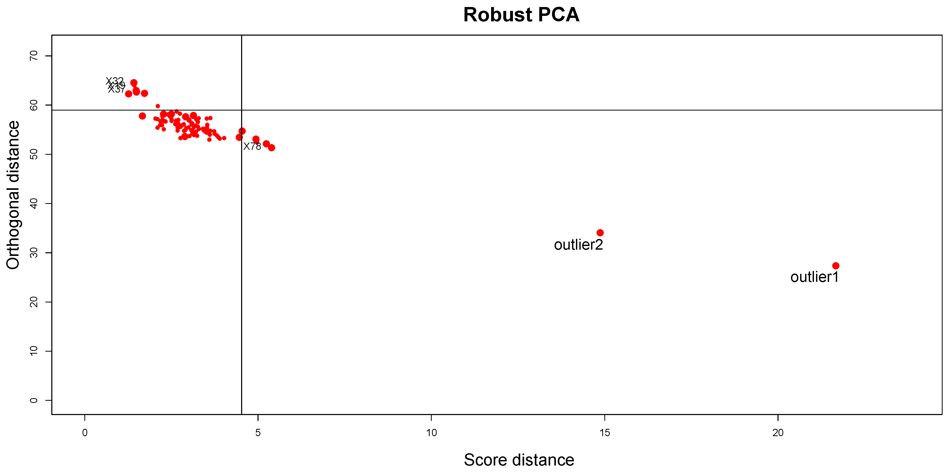
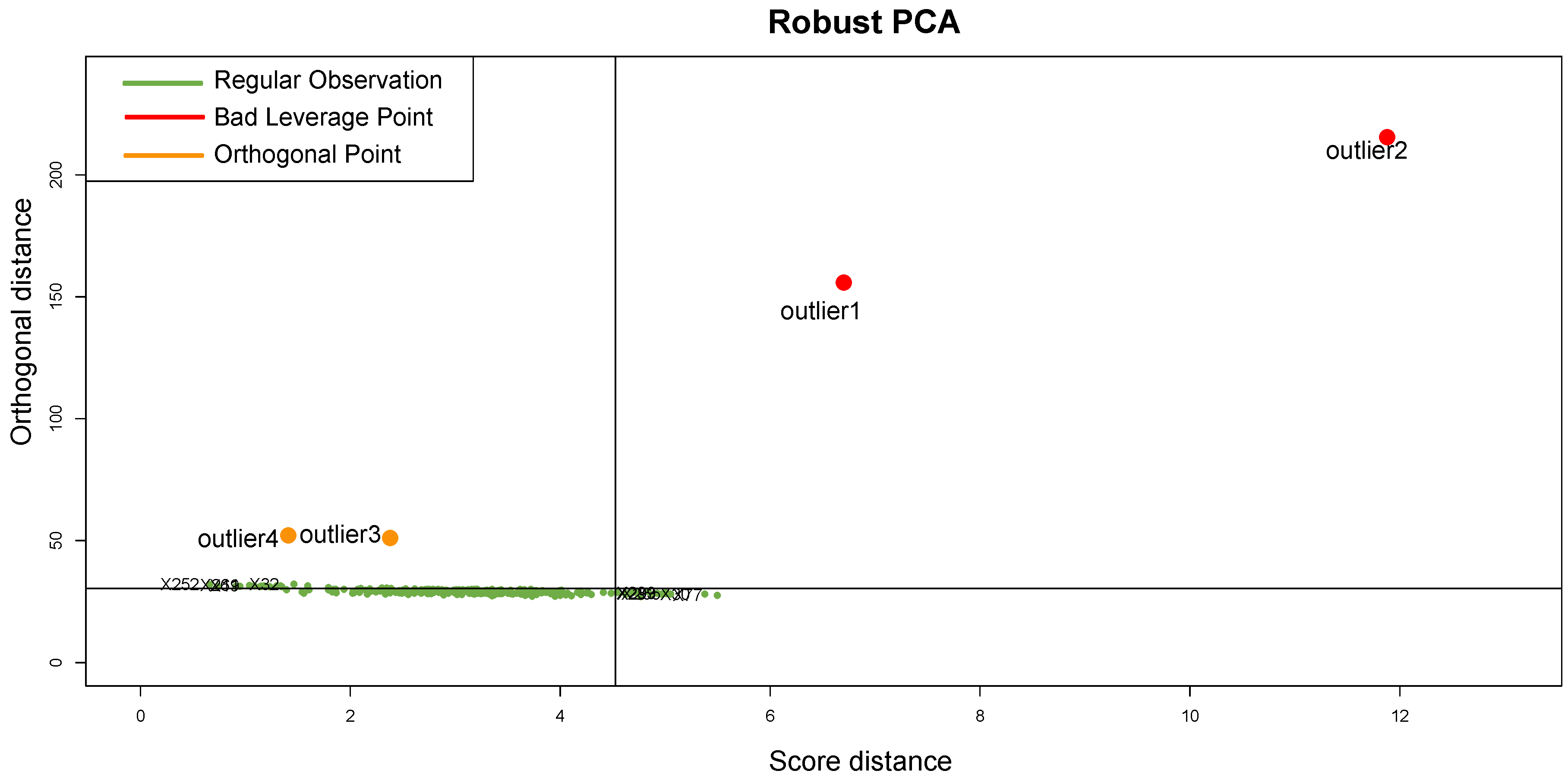
The results obtained by applying the proposed ensemble method are described below. The Silhouette coefficient is equal to $0.44$, confirming the fit of clustering to synthetic data; the CCC is equal to 0.97, confirming that the choice of Pearson distance with the Average method generates a clustering that fits to the data very well. Looking at the DD plot shown in Figure 7, one can notice that the two outliers with the t-student distribution are called BLPs, while the two samples with normal distributions different from the other samples are OOs. For a more detailed discussion of this behavior, see Section 5.

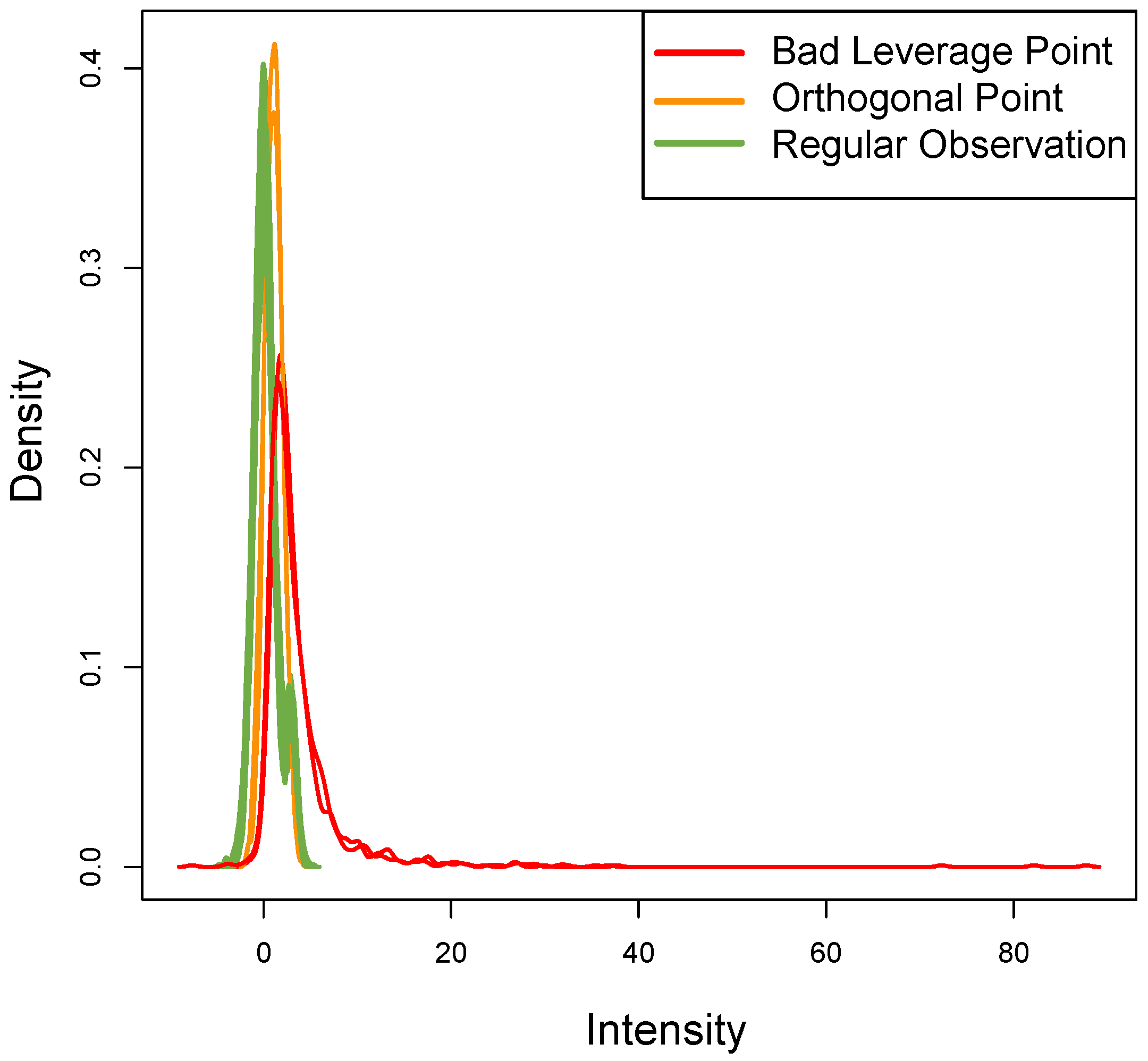
Figure 8 shows the density of each outlier sample: this plot qualitatively confirms the data assumptions above. The ROs show the typical bimodal trend present in real datasets, the OOs have a different trend but with the same distribution, while the two BLPs with t-student distribution (as expected) show a different trend.

4.2. Real Dataset

To test the effectiveness of the proposed ensemble methods in the context of microarray outlier detection, four real cancer datasets were used. These cancer datasets were selected to verify the robustness of the approach in different loading situations where either solid and biologically similar samples are outliers.

We generated four different datasets (hereafter referred to as Datasets A, B, C, and D, respectively) from real tumor gene expression profiling data characterized by patients with the same cancer type. In each dataset, we added some “true outliers” derived from patients with different cancer diagnoses, and attempted to simulate a gradient of biological distance between the “true outliers” and all other samples. Specifically, Dataset A, C, and D were added with samples derived from different tumor types or cell types, while Dataset B was added with samples having the same cell of origin of the main dataset. Specifically, Dataset A consisted of 591 samples of diffuse large B-cell lymphoma (DLBCL), a particular type of aggressive Non-Hodgkin Lymphoma (NHL) derived from B cells, and two samples of ovarian cancer (OC) [12,25,26,27,28,29,30,31].

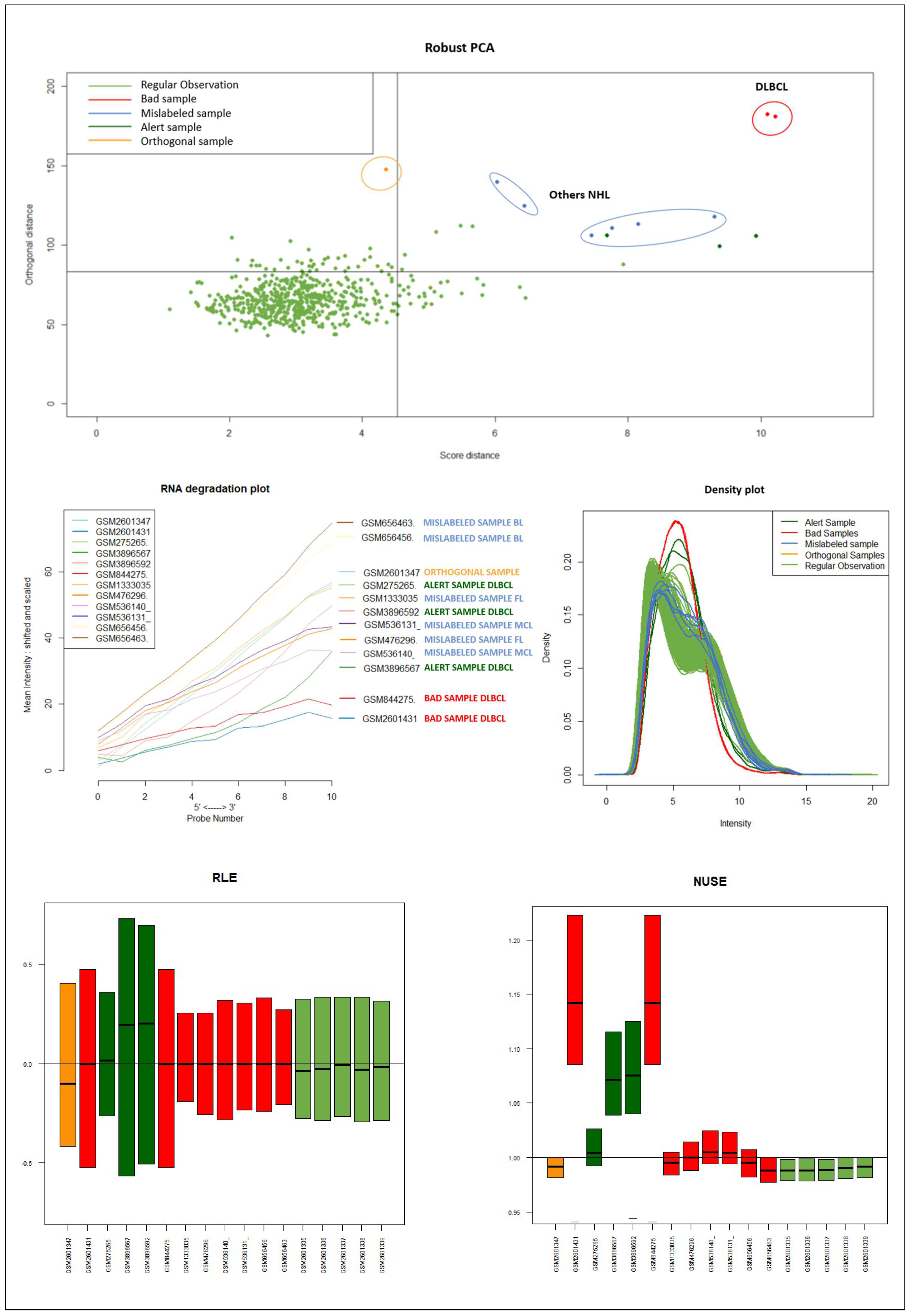
Dataset B consisted of 591 DLBCL and 6 samples of other NHL subtypes also derived from B cells (two Follicular Lymphomas FL, two Mantle Cell Lymphomas MCL , and two Burkitt Lymphoma BL) [32,33,34]. In this dataset, the choice of the Pearson’s distance is essential because the FL, MCL, and BL outliers differ little from the other samples as they come from the same type of tumor. Dataset C was created by grouping three types of hematological cancers originating from different types of hematological cells, namely 448 cases of Chronic Lymphocytic Leukemia (CLL) and three cases of T-Acute lymphoblastic leukemia (T-ALL) and three cases of Myelodysplastic Syndrome (MDS). Finally, Dataset D was created by adding three cases of breast cancer samples to 448 CLL [35].

Table 3. Description of the dataset.

	Disease	Series	References
Dataset A	DLBCL+OC	GSE10846, GSE132929, GSE23501	[12,25,26,27,28,29,30,31]
		GSE34171, GSE87371, GSE98588,
		GSE9891
Dataset B	DLBCL+FL+MCL+BL	GSE10846, GSE132929, GSE23501	[12,25,26,27,28,29]
		GSE34171, GSE87371, GSE98588,	[32,33,34]
		GSE12195, GSE55267,GSE26673
		GSE21452
Dataset C	CLL+ T-ALL+MDS	GSE13159	[35]
Dataset D	CLL+ Breast Cancer	E-MTAB-2501	[36]

summarizes the used datasets and their main characteristics.

Raw data (In particular, samples related to DLBCL are associated to GSE10846, GSE132929, GSE23501, GSE34171, GSE87371 and GSE98588; samples of ovarian cancer to GSE9891; whereas the other six samples in Dataset B were randomly chosen from GSE12195,GSE55267, GSE93261, GSE26673, and GSE21452. For the other two datasets, the baseline of 448 CLL with the particular six samples are associated to GSE13159, while the remaining three sample of breast cancer were from E-MTAB-2501 series.) were downloaded from Gene Expression Omnibus and Array Express databases and preprocessed removing background, normalizing and batch effect correction procedures (needed when raw data come from different series/laboratories). In detail, these operations allow to remove background from native files (such as CEL extension files), normalize arrays in order to have comparable samples, and correct batch effects due to systematic technical differences (such as Laboratory, time, day, or instrument used for the biological experiment [37,38,39]).

Table 4. Results obtained for each dataset. We highlight that, in Dataset C, the second cluster has seven samples instead of the expected six mislabeled samples. In the first analysis, one could think of an error in the clustering technique; in fact, the study of the degradation of the samples suggests that this sample shows a similar behavior with respect to the Normalized Unscaled Standard Error (NUSE) graph as the mislabeled samples of the cluster in which it was inserted.

	CCC	SC	Bad Leverage Points	Alert Samples	Orthogonal Outliers	Regular Observations
Dataset A	0.92	0.48	4	4	1	584
Dataset B	0.87	0.55	8	3	1	585
Dataset C	0.88	0.55	7	2	3	442
Dataset D	0.90	0.67	6	5	0	440

reports the quality metric values of clustering and the number of outliers identified in the numerical experiments, while

Table 5. Silhouette coefficient value of each dataset.

	Cluster	Size	Average Sil Width
Dataset A	1	589	0.47
	2	2	0.90
	3	2	0.56
Dataset B	1	589	0.55
	2	2	0.98
	3	6	0.42
Dataset C	1	444	0.56
	2	7	0.24
	3	1	0
	4	1	0
	5	1	0
Dataset D	1	445	0.67
	2	3	0.69
	3	1	0
	4	1	0
	5	1	0

summarizes the cardinality of each cluster and the associated averaged Silhouette (which indicates the contribution of each cluster for every dataset). High value of the CCC, as well as the values of the Silhouette coefficient, confirm the presence of a reasonable clustering structure.

It should be emphasized that the detected samples correspond to the expected outliers in all datasets (i.e., the two samples with a solid ovarian tumor in the Dataset A, the six samples divided in FL, MCL, and BL in Dataset B, three in Dataset C, and the remaining three samples of Breast cancer in Dataset D) and that the majority of them are in the quadrant of the ROBPCA and then classified as BLPs with the exception of the three samples from Dataset C, which were classified as OOs. In addition, the approach identifies other “not expected” samples as outliers: these need further investigation from a biological point of view.

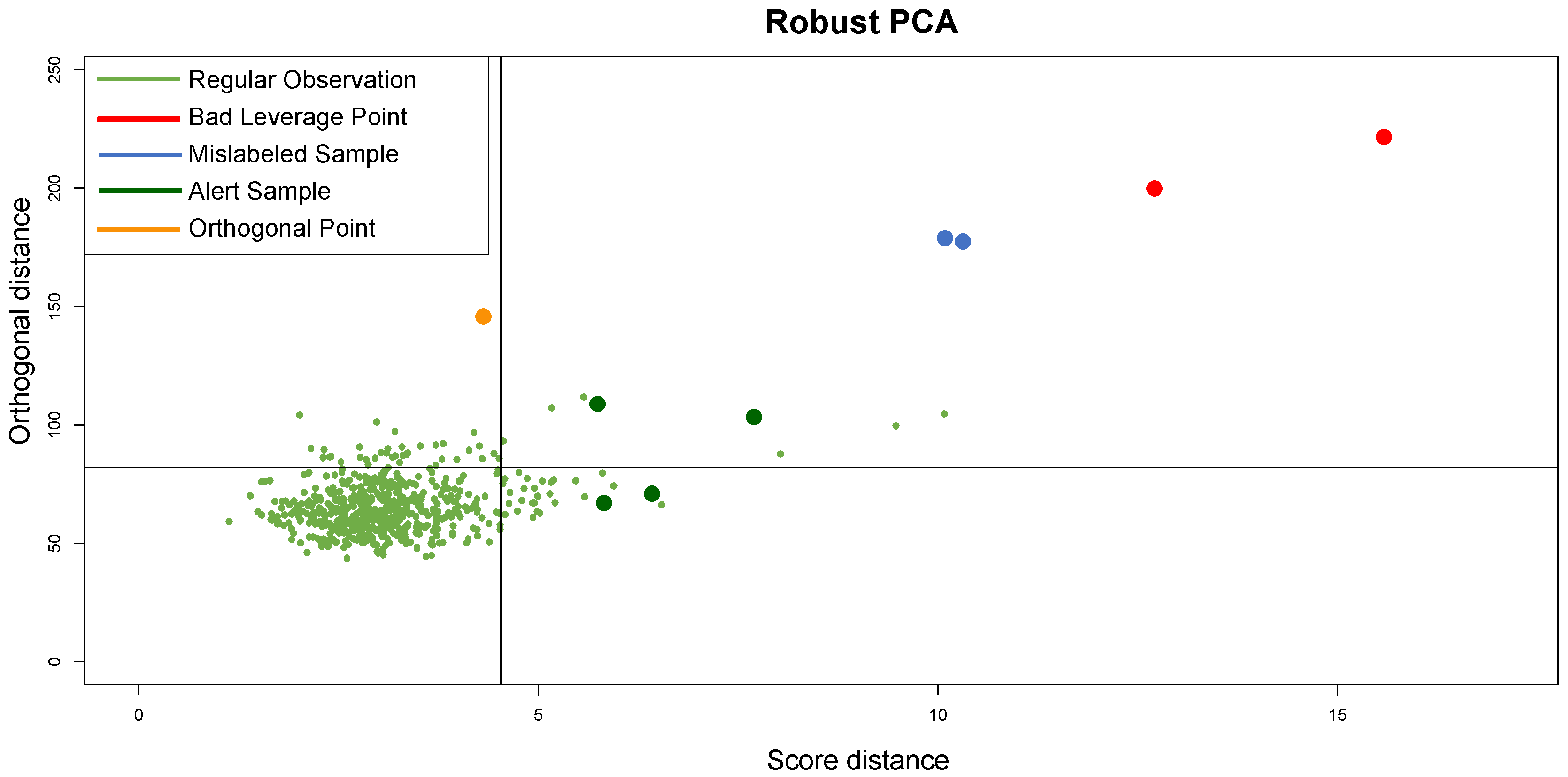
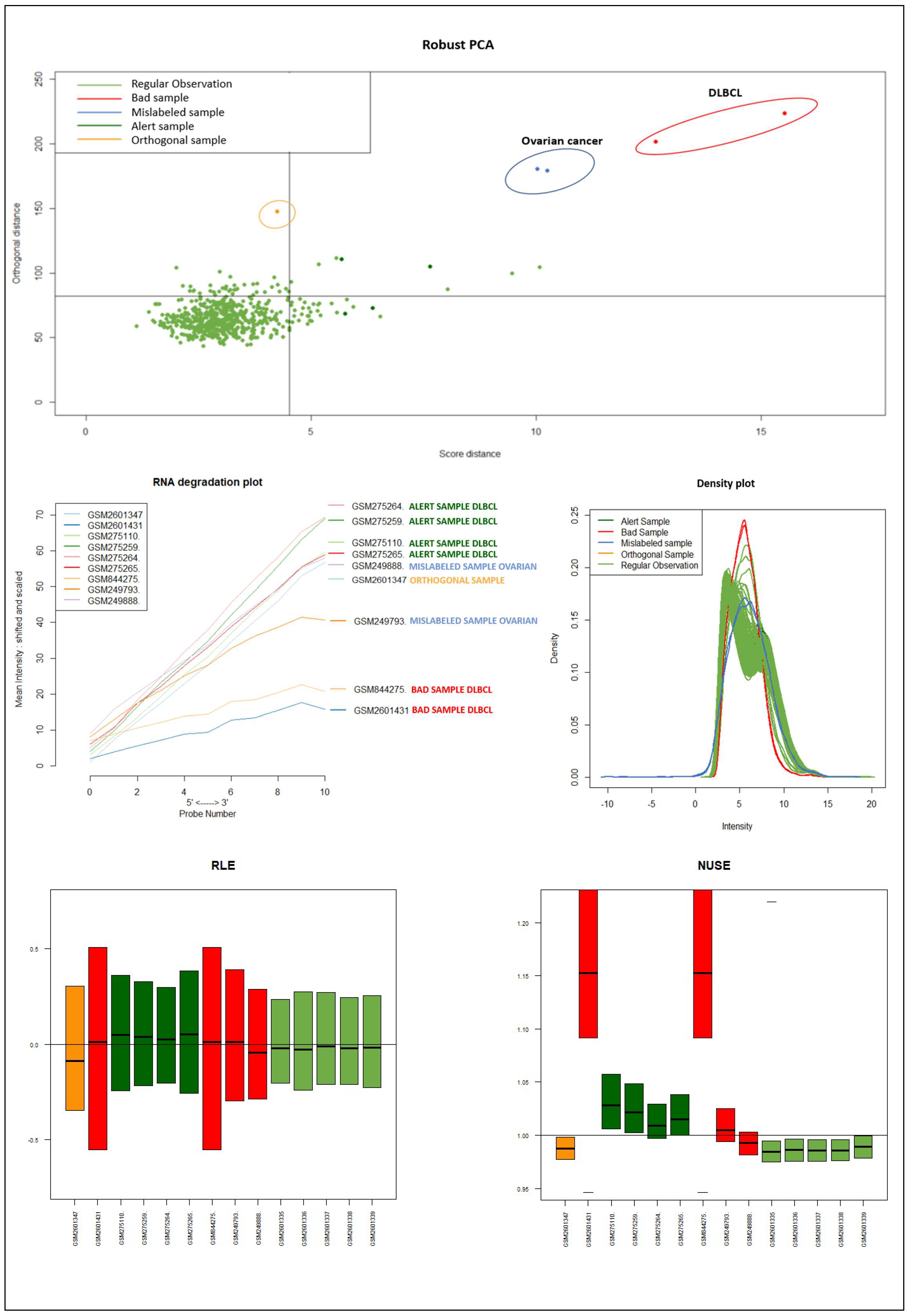
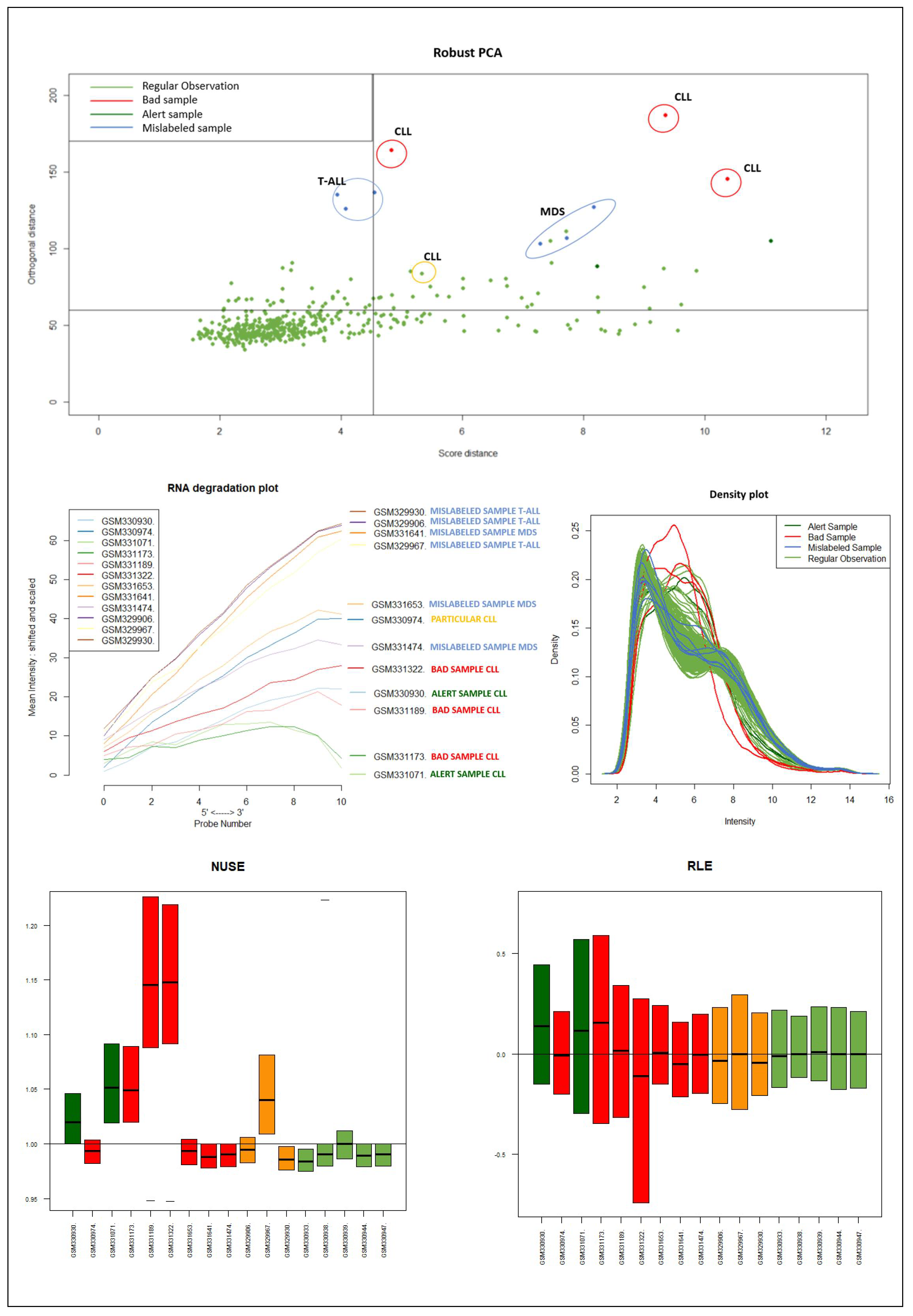
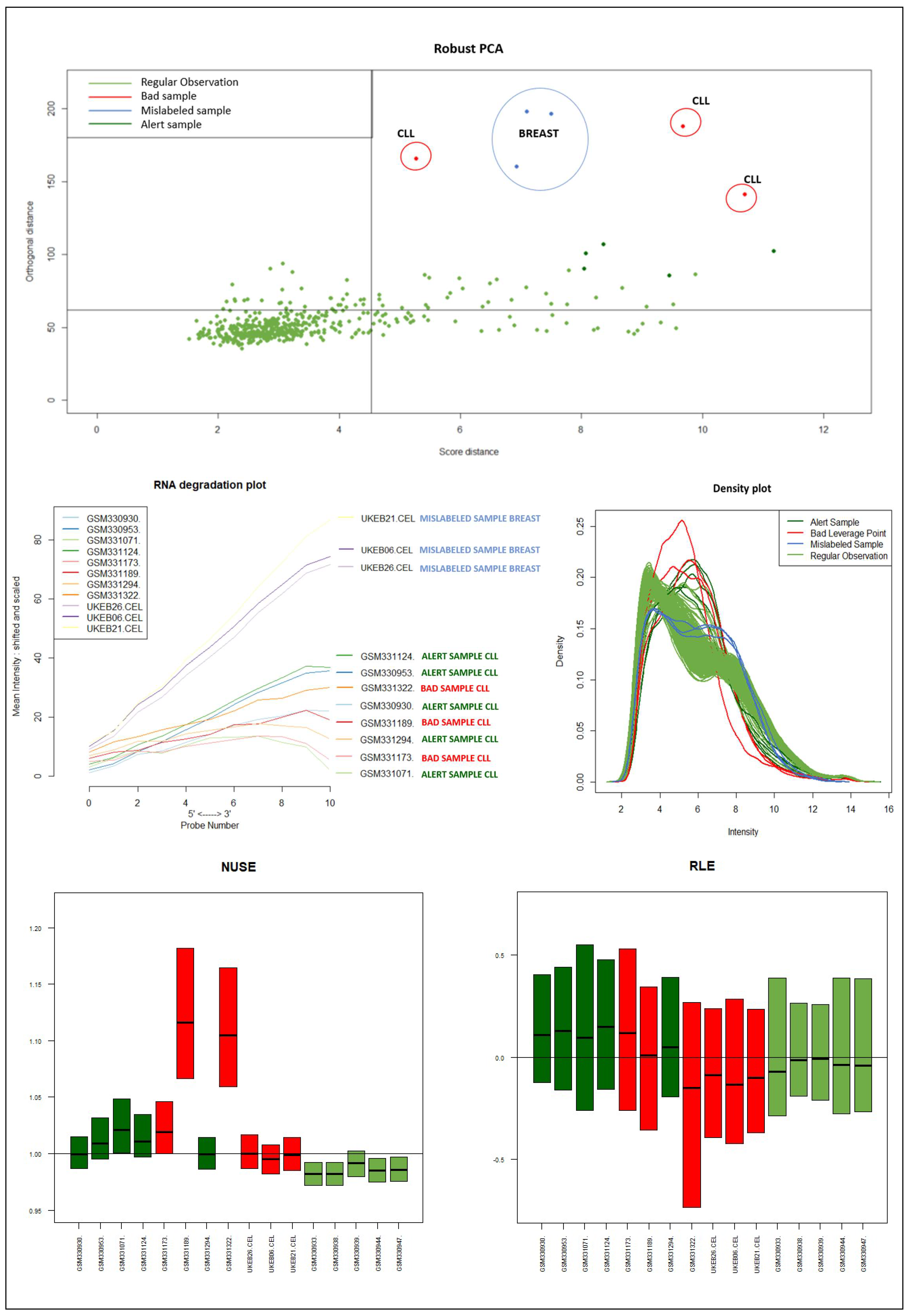
For readability, we discuss here only the results obtained when considering Dataset A, and refer the reader to the Appendix A, Appendix B, Appendix C and Appendix D for a detailed discussion of the full results for all datasets. 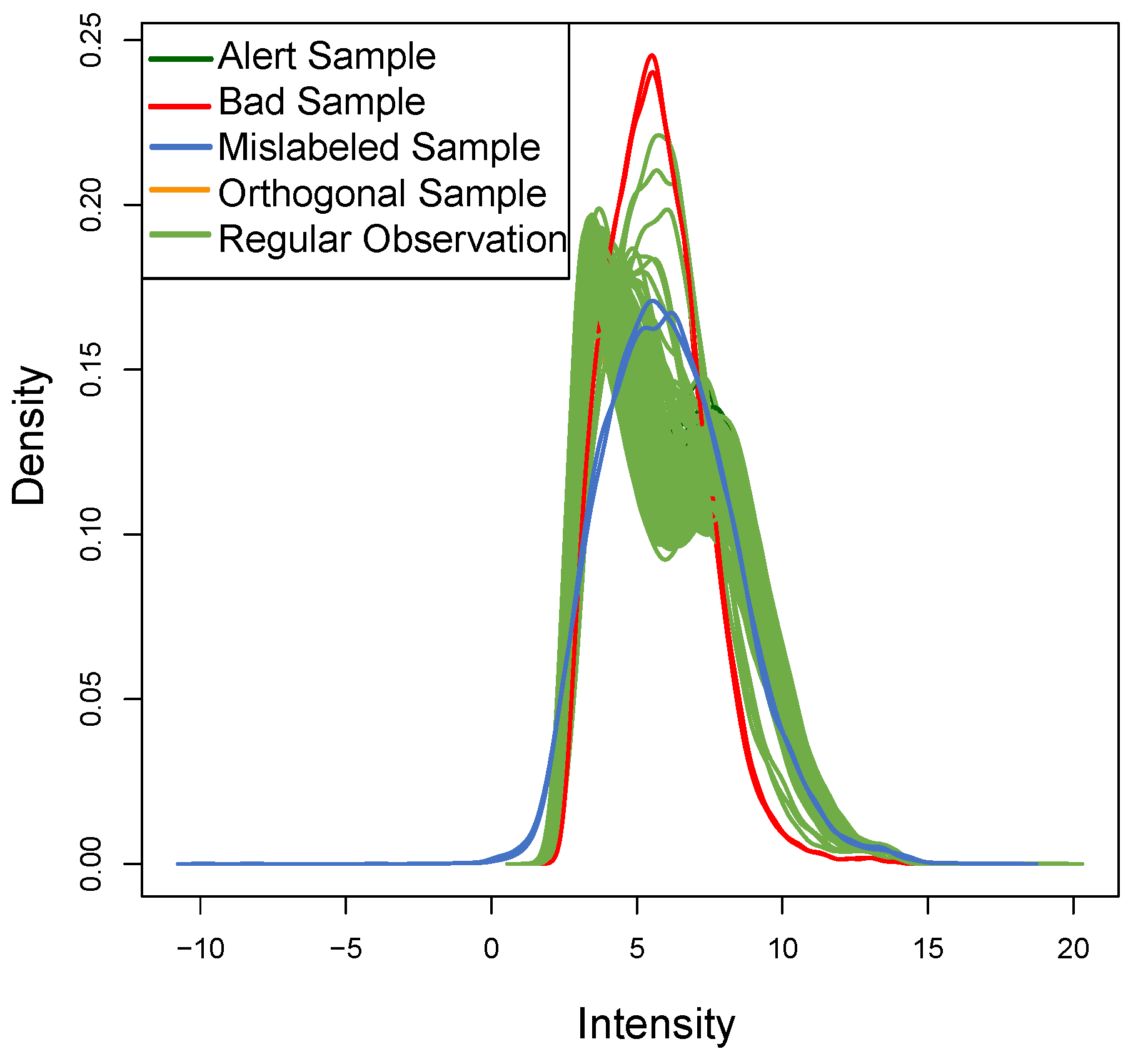Considering the distributions and positions on the DD-plot (see Figure 9) of the samples identified as novel outliers (i.e., expected a priori to be an outlier), they are correctly referred to as BLPs, ASs, and OOs. To assess the results of our approach, several density plots are performed. First, the density plot in Figure 10 illustrates the different distribution between samples labeled according to their cluster membership.

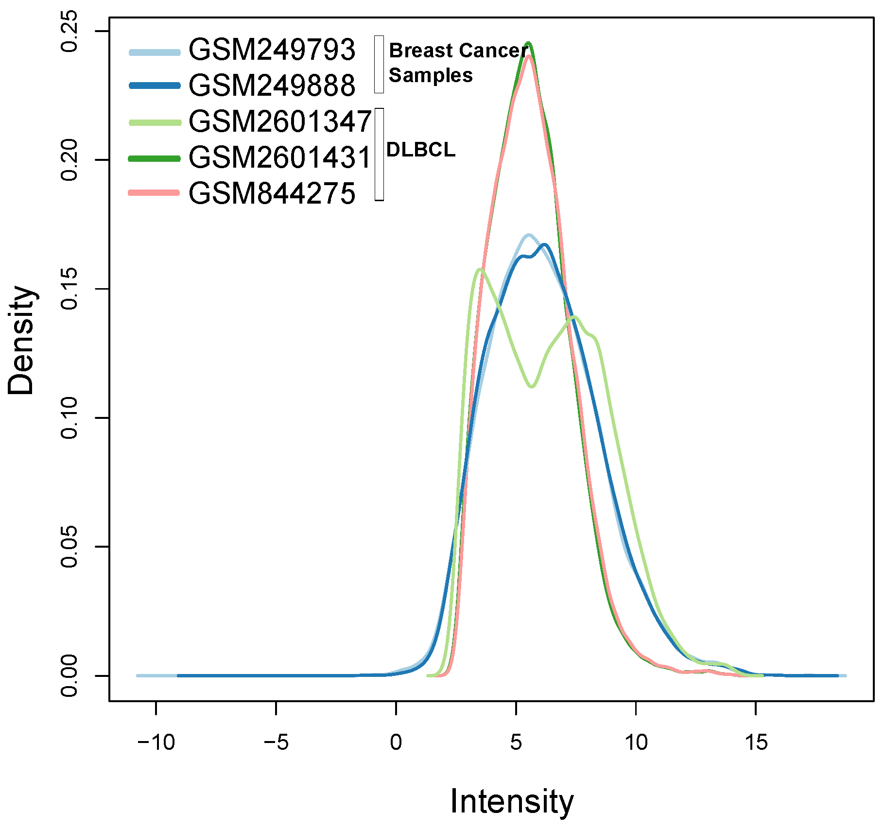
Figure 11 illustrates the density of the individual outliers obtained accordingly to their classification. The mislabeled samples (in this case the two Ovarian Cancer) are depicted in light blue and blue; BLPs are the samples in dark green and pink, whereas OOs are reported in green color.

4.3. Biological Analysis

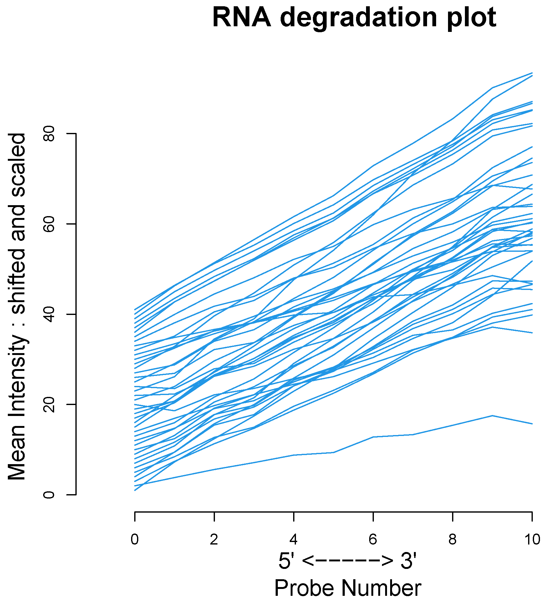
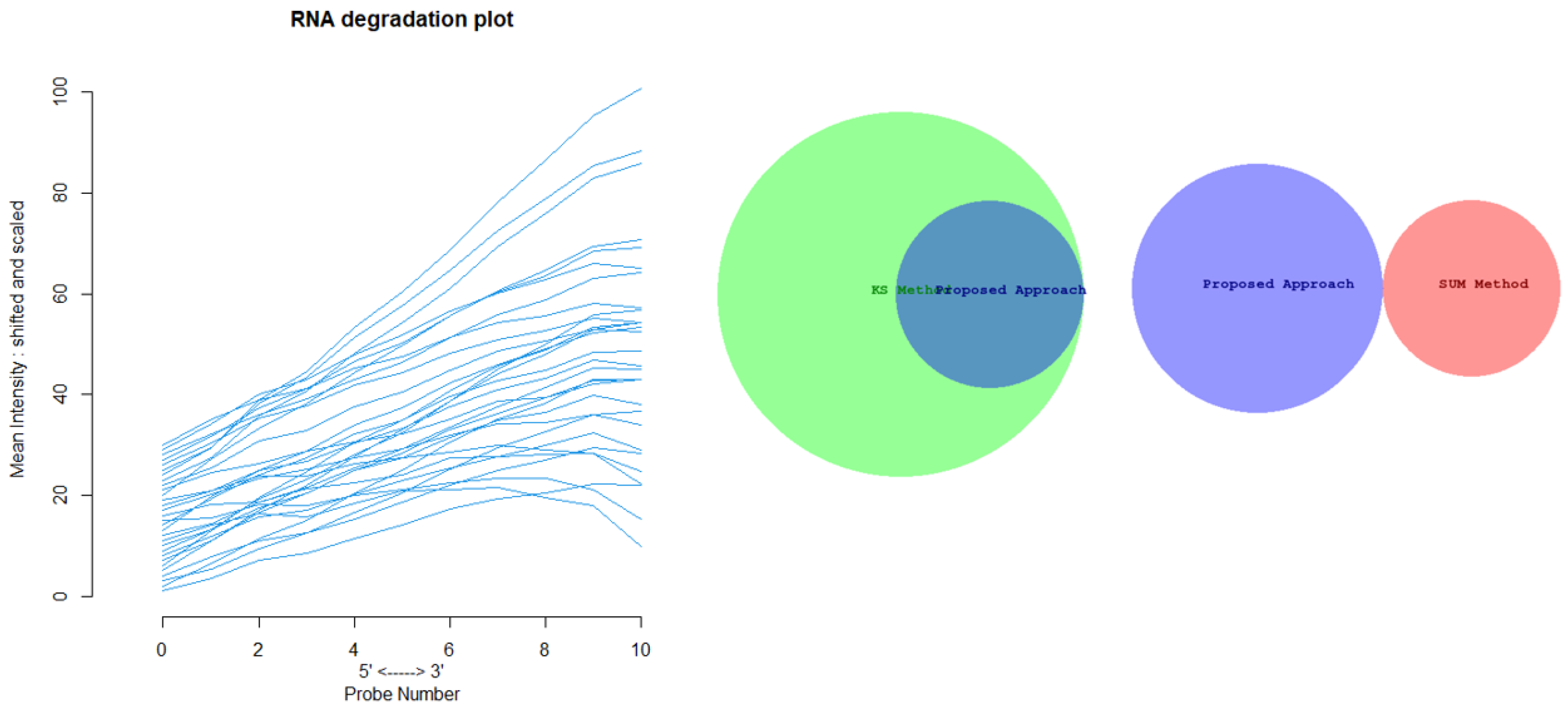
We used the four datasets to detect the outliers using both HC and Robust PCA. Interestingly, we observed that both methods were able to identify the “true outliers”; however, we also detected “unanticipated outliers” within the group of main samples. To analyze these results, we examined the array quality of each outlier by analyzing RNA degradation plots that analyze mean intensity in relation to probe numbers and help identify samples with low RNA quality; relative log expression (RLE) and Normalized Unscaled Standard Error (NUSE), implemented in the AffyRNAdeg R package. The former is calculated by subtracting the median gene expression estimate across arrays from each gene expression estimate, while the latter provides a measure of the precision of its expression estimate on a given array relative to other arrays in the batch [40]. In Dataset A, two DLBCL samples (GSM844275 and GSM2601431) were classified as BLPs along with the two “true” OC outliers and showed an irregular RNA degradation plot, NUSE and RLE, compared to the other outliers, suggesting poor array quality. Similarly, in Datasets B, the same DLBCLs were classified as BLPs, along with the FL, MCL, and BL “true outlier” samples, which instead did not show poor array quality according to RNA degradation plots, NUSE and RLE. Note that we also detected “non-expected outliers” in the CLL groups of datasets C and D, which also showed array parameters of poor quality. Interestingly, “true outliers” in Dataset C and D were characterized by good quality. We also detected OOs in Dataset A and B that were characterized by a single DLBCL case, while, in Dataset C, three MDS “true outliers” were identified as OOs outliers. All OOs showed array parameters of good quality. Finally, we identified another outlier category called “Alert” in all analyzed datasets that were displayed in the threshold range of BLPs in the DD plots, these samples were characterized by ambiguous quality array parameters. We want to specify that Alert samples are samples that may have a pre-degraded state. The algorithm signals them, and then it is up to the domain expert to verify the actual degradation state. Detailed figures regarding this point can be found in the Supplementary Materials.

4.4. Comparison with Existing Methods

To strengthen the study on the reliability of our method, we compared it with standard techniques proposed in the microarray literature (as explained in Section 2): (i) the method based on Kolmogorov-Smirnov distribution, hereafter referred to as KS, and (ii) SUM (Sum operation by column), the mechanism that assumes total weight among genes. 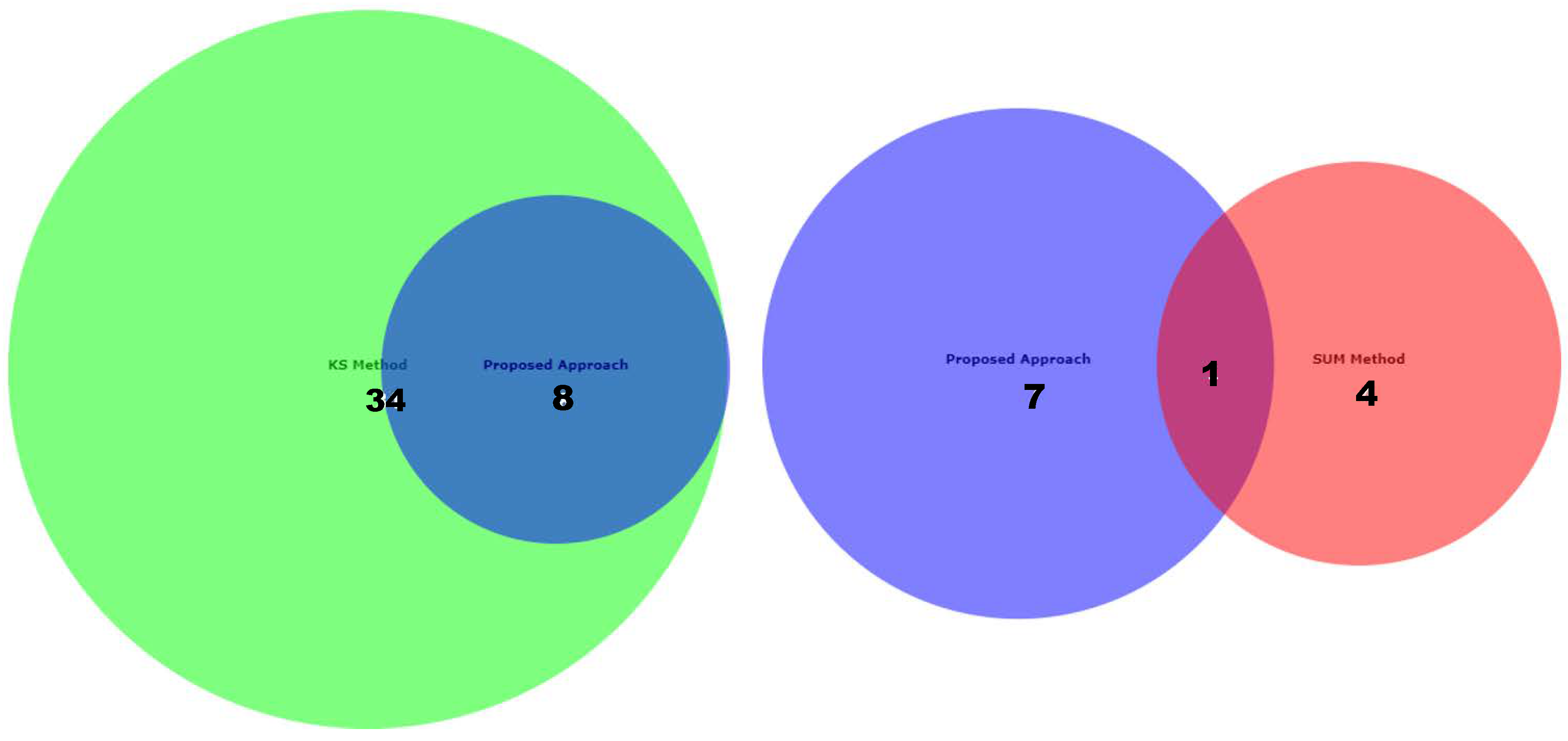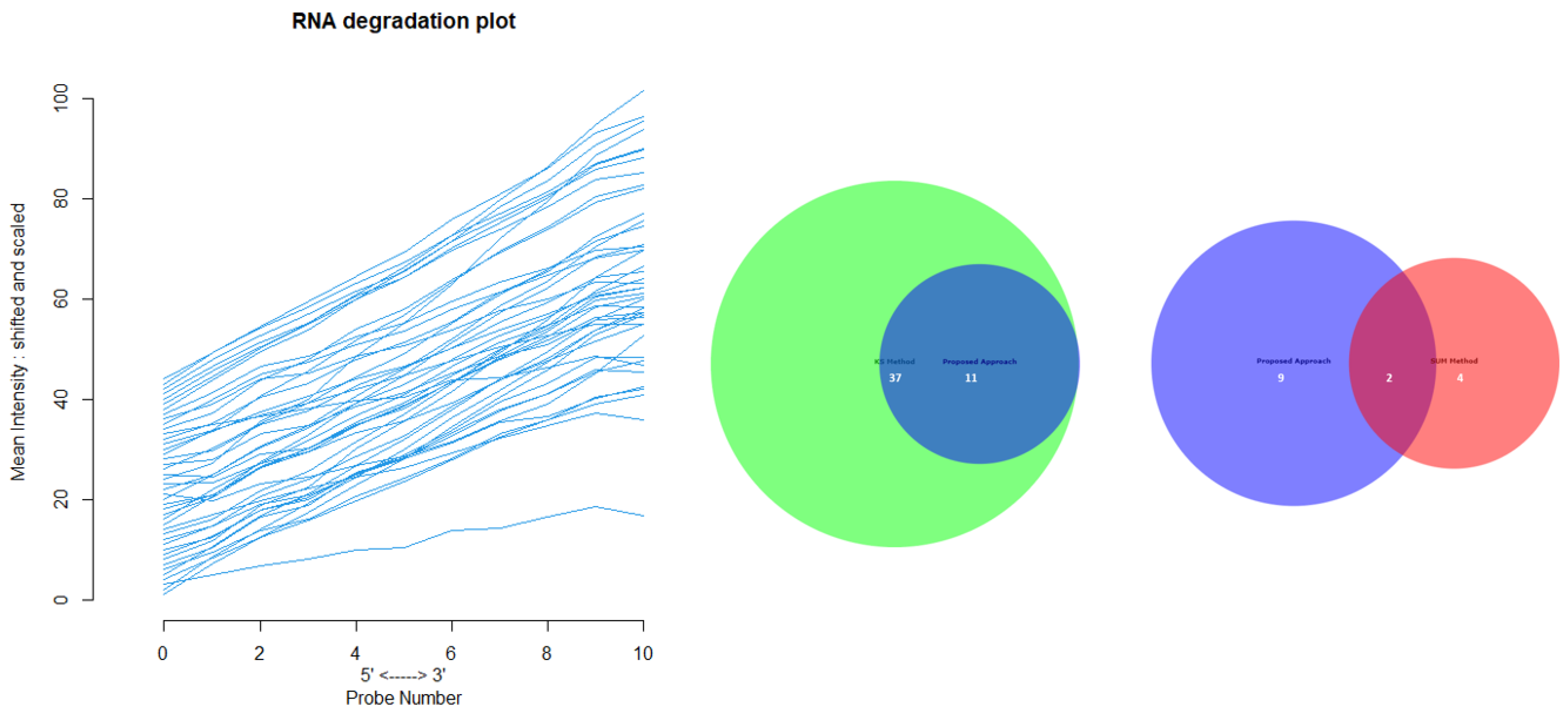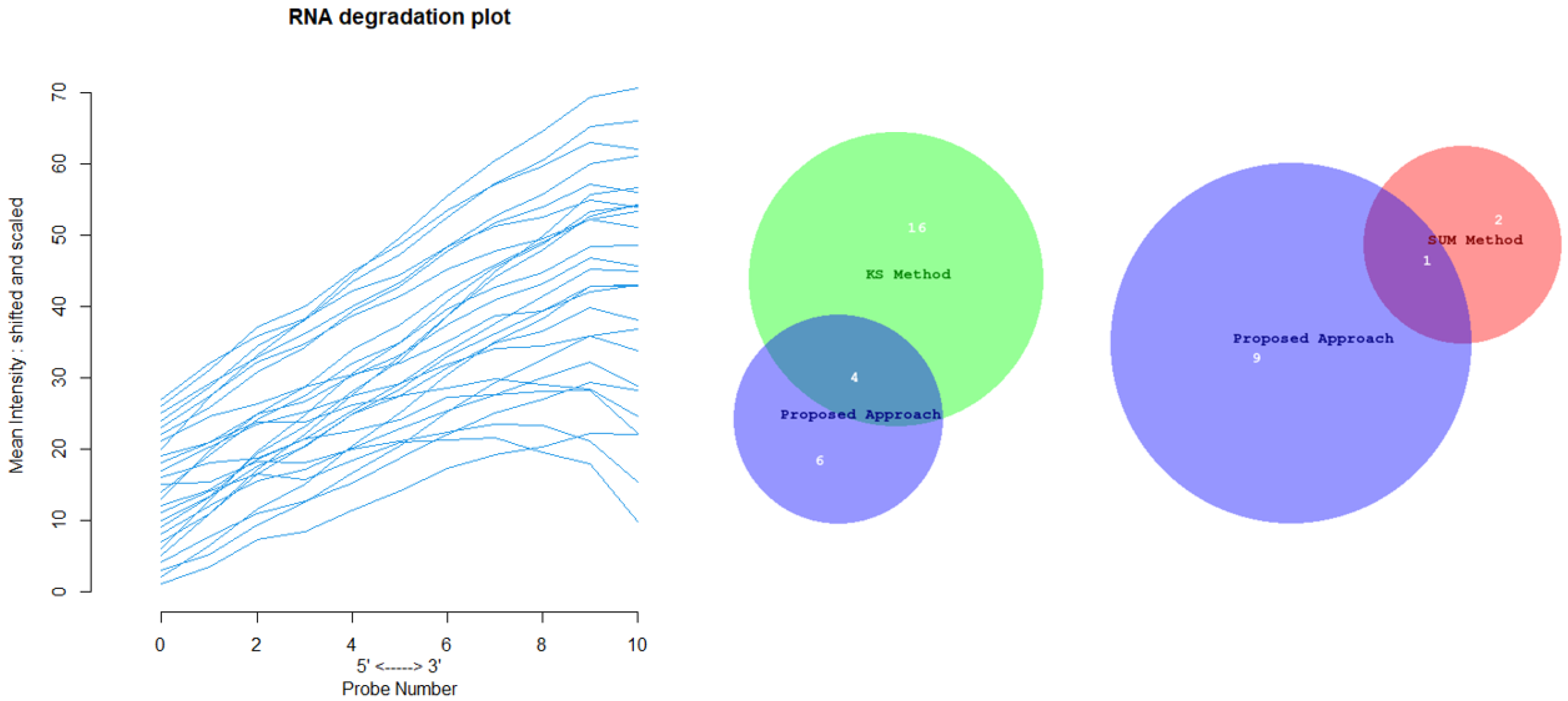As before, only the results for Datasets A are reported here (see Appendix A, Appendix B, Appendix C and Appendix D for the complete overview of all biological datasets). KS individuates 34 outliers: this is a high number compared to the nature of biological outliers, which are expected to be very small. The reason is probably that the KS procedure is based on a probability distribution distance. In contrast, SUM finds several outliers and only one outlier compared to our approach. Figure 12 shows the Euler-Venn diagram (drawn using an online tool for comparing and visualizing biological lists with area-proportional Venn diagrams) [41] for the sets of outliers detected by the three mechanisms on Dataset A, and, Figure 13 shows the study of the degradation of the additional samples obtained by the comparison techniques.

Based on these results, we can assume that our approach combines the concept of Bad Leverage points with the concept of degradation, an aspect that the other comparison techniques do not have. Indeed, it can be observed in the figure that the degraded samples are the ones identified by our approach, while the others are not degraded.

5. Discussion

An ensemble mechanism combining Robust PCA and Hierarchical Clustering with opportune distances has been proposed to search for anomalies in gene expression matrices in a more reasonable way. The strength of this method is to provide a pseudo-classification model of the outliers. Figure 14 shows a possible interpretation about the reason why each sample is in a particular quadrant of the PC plane.

The figure shows that from left to right we have the samples that have a distribution from most similar to least similar. From top to bottom, we have the samples that have a degradation status from highest to lowest. The threshold is plotted in red. According to the above discussion, we could assume that outliers that are of “low quality” are considered as very extremely bad outliers above a certain threshold. On the contrary, the “mislabeled” type outliers are on the borderline between the “orthogonal” type outliers and the bad leverage points. In general, the more the distribution of the anomalous samples deviates from the majority of the data, the more the outlier is on the right side of the plot.

From a biological perspective, our results provide a reliable tool to better understand the outlier properties. It has been widely demonstrated that a small percentage of publicly available arrays are of poor quality and that these samples can affect downstream analysis. When an outlier is detected, it is likely to be associated with poor quality values. Beyond analysis of degradation and quality data, our combined approach to outlier detection is able to identify samples with putative biological significance that may be worth investigating in terms of putative biological significance and clinical characteristics. It may also be interesting to integrate these observations with other high-throughput analyses, such as genome sequencing, to investigate what changes might be responsible for such peculiar transcriptional patterns.

By the way, a very important aspect is to establish the threshold beyond which to consider a sample degraded or not. This problem is configured as a search and optimization problem of the optimal hyperparameter [42] for which our ensemble method can be considered a possible decision model for the search for anomalies in this type of data.

6. Conclusions and Future Works

In this work, we present a new ensemble approach to anomaly detection that combines HC and Low-Rank methods. It is configured as an additional tool and allows deriving a pseudo-mathematical classification of outlier samples in GEP data focusing on microarray. Since recent work has focused only on RNA-seq data [14], we will extend our approach to be interchangeable between different platforms, such as RNA-seq and GEP from Nanostring Technologies. The preliminary experimental results performed using the proposed approach have shown that it is possible to pseudo-classify the outliers based on their nature. Future work should be carried out to identify the thresholds within which it is possible to associate the mathematically defined outlier with the biological outlier. The results obtained are quite promising and indicate the usefulness of the proposed mechanism as a preprocessing tool for the analysis of datasets that need further investigation. For example, the proposed mechanism shows that it is able to eliminate degraded samples, perform analysis on specific samples, and possibly reclassify mislabeled outlier types. Moreover, the proposed method was preliminary used in same recent prognostic studies related to LXR (Liver x receptor) protein [43], confirming its ability to identify some samples to be removed. This result helped to improve the discriminating prognosis ability of considered patient with respect to clinical outcome and the confirmed the possible applicability of the proposed procedure also in prognostic biological context.

Future research should be devoted to the construction of a new decision model that incorporates the proposed ensemble mechanism as a data preprocessing method to identify the anomalies, and integrate the anomaly detection tool into the context of microarrays for searching and classifying samples that can generate new biological hypotheses.

References

1. Moore, M.G. Introduction to the Practice of Statistics, 3rd ed.; W. H. Freeman: New York, NY, USA, 1999. [Google Scholar]
2. Rousseeuw, P.; Hubert, M. Anomaly Detection by Robust Statistics. Wiley Interdiscip. Rev. Data Min. Knowl. Discov. 2018, 8. [Google Scholar] [CrossRef] [Green Version]
3. Shieh, A.D.; Hung, Y.S. Detecting outlier samples in microarray data. Stat. Appl. Genet. Mol. Biol. 2009, 8, 13. [Google Scholar] [CrossRef] [PubMed] [Green Version]
4. Pimentel, M.A.; Clifton, D.A.; Clifton, L.; Tarassenko, L. A review of novelty detection. Signal Process. 2014, 99, 215–249. [Google Scholar] [CrossRef]
5. Thudumu, S.; Branch, P.; Jin, J.; Singh, J.J. A comprehensive survey of anomaly detection techniques for high dimensional big data. J. Big Data 2020, 7, 1–30. [Google Scholar] [CrossRef]
6. Omran, M.; Engelbrecht, A.; Salman, A. An overview of clustering methods. Intell. Data Anal. 2007, 11, 583–605. [Google Scholar] [CrossRef]
7. Bhattacharya, A.; De, R.K. A methodology for handling a new kind of outliers present in gene expression patterns. In International Conference on Pattern Recognition and Machine Intelligence; Springer: Berlin/Heidelberg, Germany, 2011; pp. 394–399. [Google Scholar]
8. Del Buono, N.; Esposito, F.; Fumarola, F.; Boccarelli, A.; Coluccia, M. Breast Cancer’s Microarray Data: Pattern Discovery Using Nonnegative Matrix Factorizations. In Machine Learning, Optimization, and Data Science. MOD 2016. Lecture Notes in Computer Science; Springer: hlBerlin/Heidelberg, Germany, 2016; Volume 10122. [Google Scholar] [CrossRef]
9. Kaufman, L.; Rousseeuw, P.J. Finding Groups in data: An Introduction to Cluster Analysis; John Wiley & Sons: Hoboken, NJ, USA, 2009; Volume 344. [Google Scholar]
10. Hubert, M.; Rousseeuw, P.J.; Vanden Branden, K. ROBPCA: A new approach to robust principal component analysis. Technometrics 2005, 47, 64–79. [Google Scholar] [CrossRef]
11. Esposito, F.; Boccarelli, A.; Del Buono, N. An NMF-Based Methodology for Selecting Biomarkers in the Landscape of Genes of Heterogeneous Cancer-Associated Fibroblast Populations. Bioinform. Biol. Insights 2020, 14. [Google Scholar] [CrossRef] [PubMed]
12. Chapuy, B.; Stewart, C.; Dunford, A.J.; Kim, J.; Kamburov, A.; Redd, R.A.; Lawrence, M.S.; Roemer, M.G.; Li, A.J.; Ziepert, M.; et al. Molecular subtypes of diffuse large B cell lymphoma are associated with distinct pathogenic mechanisms and outcomes. Nat. Med. 2018, 24, 679–690. [Google Scholar] [CrossRef]
13. Croux, C.; Filzmoser, P.; Oliveira, M. Algorithms for projection–pursuit robust principal component analysis. Chemom. Intell. Lab. Syst. 2007, 87, 218–225. [Google Scholar] [CrossRef]
14. Chen, X.; Zhang, B.; Wang, T. Robust principal component analysis for accurate outlier sample detection in RNA-Seq data. BMC Bioinform. 2020, 21. [Google Scholar] [CrossRef]
15. Kwitt, R.; Hofmann, U. Robust methods for unsupervised PCA-based anomaly detection. In Proceedings of the IEEE/IST WorNshop on Monitoring, AttacN Detection and Mitigation, Tuebingen, Germany, 28–29 September 2006; pp. 1–3. [Google Scholar]
16. Jolliffe, I.T.; Jorge, C. Principal component analysis: A review and recent developments. Philos. Trans. R. Soc. A 2016. [Google Scholar] [CrossRef]
17. Choi, Y.; Taylor, J.; Tibshirani, R. Selecting the number of principal components: Estimation of the true rank of a noisy matrix. Ann. Stat. 2017, 45, 2590–2617. [Google Scholar] [CrossRef]
18. Hung, H.; Huang, S.Y.; Ing, C.K. A generalized information criterion for high-dimensional PCA rank selection. arXiv 2020, arXiv:2004.13914. [Google Scholar]
19. Paquet, A.; Yang, J. arrayQuality: Assessing Array Quality on Spotted Arrays. 2020. Available online: http://arrays.ucsf.edu/ (accessed on 5 November 2020).
20. Kauffmann, A.; Gentleman, R.; Huber, W. arrayQualityMetrics—A bioconductor package for quality assessment of microarray data. Bioinformatics 2009, 25, 415–416. [Google Scholar] [CrossRef] [PubMed] [Green Version]
21. R Core Team. R: A Language and Environment for Statistical Computing; R Foundation for Statistical Computing: Vienna, Austria, 2015. [Google Scholar]
22. Cui, H.; Zheng, M.; Zhao, G.; Liu, R.; Wen, J. Identification of differentially expressed genes and pathways for intramuscular fat metabolism between breast and thigh tissues of chickens. BMC Genom. 2018, 19, 55. [Google Scholar] [CrossRef] [PubMed]
23. Shinmura, S. High-Dimensional Microarray Data Analysis; Springer: Berlin/Heidelberg, Germany, 2019. [Google Scholar]
24. Barghash, A.; Arslan, T.; Helms, V. Robust detection of outlier samples and genes in expression datasets. J. Proteom. Bioinform. 2016, 9, 38–48. [Google Scholar] [CrossRef] [Green Version]
25. Bethge, N.; Honne, H.; Hilden, V.; Trøen, G.; Eknæs, M.; Liestøl, K.; Holte, H.; Delabie, J.; Smeland, E.B.; Lind, G.E. Identification of highly methylated genes across various types of B-cell non-hodgkin lymphoma. PLoS ONE 2013, 8, e79602. [Google Scholar] [CrossRef] [Green Version]
26. Shaknovich, R.; Geng, H.; Johnson, N.A.; Tsikitas, L.; Cerchietti, L.; Greally, J.M.; Gascoyne, R.D.; Elemento, O.; Melnick, A. DNA methylation signatures define molecular subtypes of diffuse large B-cell lymphoma. Blood J. Am. Soc. Hematol. 2010, 116, e81–e89. [Google Scholar] [CrossRef] [Green Version]
27. Monti, S.; Chapuy, B.; Takeyama, K.; Rodig, S.J.; Hao, Y.; Yeda, K.T.; Inguilizian, H.; Mermel, C.; Currie, T.; Dogan, A.; et al. Integrative analysis reveals an outcome-associated and targetable pattern of p53 and cell cycle deregulation in diffuse large B cell lymphoma. Cancer Cell 2012, 22, 359–372. [Google Scholar] [CrossRef] [Green Version]
28. Dubois, S.; Viailly, P.J.; Bohers, E.; Bertrand, P.; Ruminy, P.; Marchand, V.; Maingonnat, C.; Mareschal, S.; Picquenot, J.M.; Penther, D.; et al. Biological and clinical relevance of associated genomic alterations in MYD88 L265P and non-L265P–mutated diffuse large B-cell lymphoma: Analysis of 361 cases. Clin. Cancer Res. 2017, 23, 2232–2244. [Google Scholar] [CrossRef] [Green Version]
29. Tothill, R.W.; Tinker, A.V.; George, J.; Brown, R.; Fox, S.B.; Lade, S.; Johnson, D.S.; Trivett, M.K.; Etemadmoghadam, D.; Locandro, B.; et al. Novel molecular subtypes of serous and endometrioid ovarian cancer linked to clinical outcome. Clin. Cancer Res. 2008, 14, 5198–5208. [Google Scholar] [CrossRef] [PubMed] [Green Version]
30. Pasqualucci, L.; Dominguez-Sola, D.; Chiarenza, A.; Fabbri, G.; Grunn, A.; Trifonov, V.; Kasper, L.H.; Lerach, S.; Tang, H.; Ma, J.; et al. Inactivating mutations of acetyltransferase genes in B-cell lymphoma. Nature 2011, 471, 189–195. [Google Scholar] [CrossRef] [PubMed] [Green Version]
31. Guo, S.; Chan, J.K.; Iqbal, J.; McKeithan, T.; Fu, K.; Meng, B.; Pan, Y.; Cheuk, W.; Luo, D.; Wang, R.; et al. EZH2 mutations in follicular lymphoma from different ethnic groups and associated gene expression alterations. Clin. Cancer Res. 2014, 20, 3078–3086. [Google Scholar] [CrossRef] [PubMed] [Green Version]
32. Huet, S.; Tesson, B.; Jais, J.P.; Feldman, A.L.; Magnano, L.; Thomas, E.; Traverse-Glehen, A.; Albaud, B.; Carrère, M.; Xerri, L.; et al. A gene-expression profiling score for prediction of outcome in patients with follicular lymphoma: A retrospective training and validation analysis in three international cohorts. Lancet Oncol. 2018, 19, 549–561. [Google Scholar] [CrossRef] [Green Version]
33. Piccaluga, P.P.; De Falco, G.; Kustagi, M.; Gazzola, A.; Agostinelli, C.; Tripodo, C.; Leucci, E.; Onnis, A.; Astolfi, A.; Sapienza, M.R.; et al. Gene expression analysis uncovers similarity and differences among Burkitt lymphoma subtypes. Blood 2011, 117, 3596–3608. [Google Scholar] [CrossRef] [Green Version]
34. Hartmann, E.M.; Campo, E.; Wright, G.; Lenz, G.; Salaverria, I.; Jares, P.; Xiao, W.; Braziel, R.M.; Rimsza, L.M.; Chan, W.C.; et al. Pathway discovery in mantle cell lymphoma by integrated analysis of high-resolution gene expression and copy number profiling. Blood J. Am. Soc. Hematol. 2010, 116, 953–961. [Google Scholar] [CrossRef] [PubMed]
35. Kohlmann, A.; Kipps, T.J.; Rassenti, L.Z.; Downing, J.R.; Shurtleff, S.A.; Mills, K.I.; Gilkes, A.F.; Hofmann, W.K.; Basso, G.; Dell’Orto, M.C.; et al. An international standardization programme towards the application of gene expression profiling in routine leukaemia diagnostics: The Microarray Innovations in LEukemia study prephase. Br. J. Haematol. 2008, 142, 802–807. [Google Scholar] [CrossRef]
36. Werner, S.; Brors, B.; Eick, J.; Marques, E.; Pogenberg, V.; Parret, A.; Kemming, D.; Ylstra, B.; Wood, A.W.; Edgren, H.; et al. RAI2 is involved in early Dissemination and Differentiation of Breast. Cancer 2015, 5, 466–468. [Google Scholar]
37. Leek, J.T.; Scharpf, R.B.; Bravo, H.C.; Simcha, D.; Langmead, B.; Johnson, W.E.; Geman, D.; Baggerly, K.; Irizarry, R.A. Tackling the widespread and critical impact of batch effects in high-throughput data. Nat. Rev. Genet. 2010, 11, 733–739. [Google Scholar] [CrossRef] [PubMed] [Green Version]
38. Leek, J.T.; Johnson, W.E.; Parker, H.S.; Jaffe, A.E.; Storey, J.D. The sva package for removing batch effects and other unwanted variation in high-throughput experiments. Bioinformatics 2012, 28, 882–883. [Google Scholar] [CrossRef]
39. Johnson, W.E.; Li, C.; Rabinovic, A. Adjusting batch effects in microarray expression data using empirical Bayes methods. Biostatistics 2007, 8, 118–127. [Google Scholar] [CrossRef] [PubMed]
40. McCall, M.N.; Murakami, P.N.; Lukk, M.; Huber, W.; Irizarry, R.A. Assessing affymetrix GeneChip microarray quality. BMC Bioinform. 2011, 12, 137. [Google Scholar] [CrossRef] [PubMed] [Green Version]
41. Hulsen, T.; de Vlieg, J.; Alkema, W. BioVenn—A web application for the comparison and visualization of biological lists using area-proportional Venn diagrams. BMC Genom. 2008, 9, 488. [Google Scholar] [CrossRef] [PubMed] [Green Version]
42. Selicato, L.; Del Buono, N.; Esposito, F. Methods for Hyperparameters Optimization in Learning Approaches: An overview. In Machine Learning, Optimization, and Data Science. LOD 2020. Lecture Notes in Computer Science; Springer: Berlin/Heidelberg, Germany, 2020; Volume 12514. [Google Scholar] [CrossRef]
43. Vegliante, M.; De Summa, S.; Fabbri, M.; Opinto, G.; Melle, F.; Motta, G.; Gulino, A.; Loseto, G.; Minoia, C.; Tommasi, S.; et al. PF510 A 14-Gene signature associated to cholesterol metabolism identifies M1-like tumor-infiltrating macrophages and predicts patient survival in diffuse Large B Cell Lymphoma. HemaSphere 2019, 3, 208. [Google Scholar] [CrossRef]
Figure 1. Graphical representation of the outlier classification (with p = 3 and k = 2 ) according to the location of each observation with respect to the PCA subspace.
Mathematics 09 00882 g001
Figure 2. Outlier map created using Robust Principal Component Analysis (ROBPCA) (Rospca package available in the R environment) on a simulated dataset. Based on the previous classification, the first quadrant (top-right) of the DD-plot (Distance-Distance plot) contains the BLPs, the second quadrant (top-left) encloses the OOs, the third quadrant (bottom-left) has the ROs, and, finally, the fourth quadrant (bottom-right) contains the GLPs.
Mathematics 09 00882 g002
Figure 3. Workflow of the proposed ensemble approach for detecting anomalies in gene expression matrices. The input data matrix firstly undergoes to Hierarchical Clustering (R package eclust) which provides the intermediate output. Then, Robust PCA (R package rospca) is applied to derive the final characterized nature of anomalies as described in Algorithm 1. The labels reported in the figure referred to: R = Regular Observation, O ¯ = Outier, O = Orthogonal Outlier, B = Bad Leverage Point, A = Alert Sample type.
Mathematics 09 00882 g003
Figure 4. The heatmap of the first synthetic dataset, sizing 1000 × 100 , in which rows and columns ideally correspond to genes and samples, respectively. The map evidences the changes of samples 10, 15, and 20 of class C 1 with samples 60, 65, and 70 of class C 2 and the different distribution of last sample of each class into the 100 last rows of the data matrix.
Mathematics 09 00882 g004
Figure 5. Circular dendrogram of first artificial dataset. The two classes are clustered correctly, respectively, in blue and in red. From the graph, it can be seen that the samples moved from one class to another (in the labels underlined with the word “shift”) are repositioned in the correct class. The two samples with different distribution are in green.
Mathematics 09 00882 g005
Figure 6. DD-plot of the first simulated dataset.
Mathematics 09 00882 g006
Figure 7. DD-plot of the second synthetic dataset. The two BLPs are in red in the top-right quadrant, and the two OOs are in orange in the top-left quadrant.
Mathematics 09 00882 g007
Figure 8. Density plot of samples of second synthetic dataset, grouped by clustering.
Mathematics 09 00882 g008
Figure 9. DD-plot of Dataset A. The two BLPs (in red) and the two mislabeled samples (in blue) are in the top-right quadrant, the OO (in orange) are in the top-left quadrant, and some ASs (dark green) are on the border between the top-right quadrant and the bottom-right quadrant.
Mathematics 09 00882 g009
Figure 10. Density Plot of samples of Dataset A, grouped by classification.
Mathematics 09 00882 g010
Figure 11. Outliers Density Plot of Dataset A.
Mathematics 09 00882 g011
Figure 12. Euler-Venn diagrams comparing the results obtained by the three methods for Dataset A.
Mathematics 09 00882 g012
Figure 13. Degradation plot of outliers obtained by Kolmogorov-Smirnov (KS) and SUM techniques applied on Dataset A.
Mathematics 09 00882 g013
Figure 14. Pseudo-classification of the outlier position.
Mathematics 09 00882 g014