Why Improving the Accuracy of Exponential Integrators Can Decrease Their Computational Cost?

Abstract

In previous papers, a technique has been suggested to avoid order reduction when integrating initial boundary value problems with several kinds of exponential methods. The technique implies in principle to calculate additional terms at each step from those already necessary without avoiding order reduction. The aim of the present paper is to explain the surprising result that, many times, in spite of having to calculate more terms at each step, the computational cost of doing it through Krylov methods decreases instead of increases. This is very interesting since, in that way, the methods improve not only in terms of accuracy, but also in terms of computational cost.

1. Introduction

Exponential methods have become a valuable tool to integrate initial boundary value problems due to the recent development of techniques which allow us to calculate exponential-type functions in a more efficient way. From the paper in [1] to that in [2] twenty-five years later, some advances were made. However, apart from that, Krylov methods have become especially interesting in the context of the space discretization of boundary value problems because the matrices which turn up there are sparse. These iterative methods reduce the computation of an exponential-type function of those large matrices applied over a certain vector to the computation of a function of a much smaller matrix. In that sense, not only polynomial Krylov methods [3,4,5,6,7,8,9,10] have been considered, but also rational Krylov methods [11,12,13,14,15,16,17,18], which lead to a much better convergence rate, but imply to solve linear systems during the iteration process.

On the other hand, exponential methods were first introduced and analysed for the case of homogeneous boundary conditions [19]. Even in that case, order reduction is observed with respect to their classical counterparts unless more stringent conditions of annihilation on the boundary or periodic boundary conditions are considered (see [20,21] for the analysis with Lawson methods and [22] for splitting ones). With exponential Runge–Kutta methods, stiff order conditions have been derived [23] which may increase the number of stages which are necessary to get a given order.

In order to avoid order reduction with all these methods (without increasing the number of stages and even for time-dependent boundary conditions), some techniques have been suggested in [24,25,26,27,28,29,30]. What we have observed in some numerical experiments with the techniques in those papers is that, when avoiding order reduction, it does not only happen that the error diminishes more quickly with the stepsize, but also that, for a same moderate stepsize, the error is smaller and, what is more impressive, that the computational cost for a same stepsize is smaller. This is striking because increasing the order of the method implies calculating more terms at each step. However, by using the Krylov subroutine phipm.m in [8] in MATLAB to calculate those terms, we have checked in some cases that the computational cost is reduced. More precisely, Figure 6.1 in [30] shows this phenomenon when avoiding order reduction with a second-order Lawson method and Figure 1 [28] does the same with a second-order exponential Runge–Kutta method.

The aim of the paper is to understand why that reduction in computational cost for a same stepsize happens when avoiding order reduction. For that, we centre on symmetric discretizations of the differential operator of the problem at hand. Moreover, we will consider both the standard Krylov method and the purely rational Krylov one.

The paper is structured as follows. Section 2 gives some preliminaries on the problem to integrate and the technique to avoid order reduction. In Section 3, the standard Krylov technique and the commonly used adaptive subroutine phipm.m is described. It is then analysed how the subroutine works when the technique to avoid order reduction is applied in the naive way. Then, another more clever way to apply the same subroutine is suggested, as well as an improvement of the subroutine for the case at hand. Finally, in Section 4, the behaviour of the purely rational Krylov method is also studied when applied inside the technique to avoid order reduction, and it is again justified that increasing the order (and therefore accuracy) may be cheaper than not doing it. The main conclusions are stated in Section 5.

2. Preliminaries

The technique in [21,24,25,26,27,29,30] to avoid order reduction when integrating linear and non-linear initial boundary value problems with exponential splitting, Lawson and Runge–Kutta methods is based on applying the method of lines in the reverse order than usual: Integrating firstly in time and then in space.

More precisely, we assume that the problem to integrate is

$$\begin{array}{c}\hfill \begin{array}{ccc}\hfill u^{\prime }\left(t\right)& =& Au\left(t\right)+f(t,u(t\left)\right),0\le t\le T,\hfill \\ \hfill u\left(0\right)& =& u_0\in X,\hfill \\ \hfill \partial u\left(t\right)& =& g\left(t\right)\in Y,0\le t\le T,\hfill \end{array}\end{array}$$

(1)

where ’ corresponds to differentiation with respect to time, X and Y are function spaces, $\partial :D\left(A\right)\subset X\to Y$ corresponds to a boundary operator, $A:D\left(A\right)\to X$ to a differential space operator, and $f:[0,T]\times D\left(A\right)\to X$ is a smooth source term. For a more detailed description of the assumptions, look at [21,24,25,26,27,29,30]. When considering the time integration of this problem with exponential methods, exponential-type functions turn up. We remind that ${\phi }_0\left(z\right)=e^z$, and that, for $j\ge 1$,

$$\begin{array}{c}\hfill {\phi }_j\left(z\right)=\frac{1}{(j-1)!}{\int }_0^1{e}^{z(1-u)}{u}^{j-1}du.\end{array}$$

(2)

For example, ${\phi }_1\left(z\right)=(e^z-1)/z$, ${\phi }_2\left(z\right)=(e^z-1-z)/z^2$. Then, as the exponentials and ${\phi }_j$-functions should be applied over a differential operator instead of a matrix, those terms were suggested to be substituted by the solution of initial boundary value problems with appropriate boundaries. More precisely, $e^{\tau A}\alpha$ has been understood as the solution of problem

$$\begin{array}{ccc}\hfill v^{\prime }\left(\tau \right)& =& Av\left(\tau \right),\hfill \\ \hfill v\left(0\right)& =& \alpha ,\hfill \\ \hfill \partial vs.\left(\tau \right)& =& \partial \left(\sum _{l=0}^r\frac{{\tau }^l}{l!}{A}^l\alpha \right),\hfill \end{array}$$

(3)

when $\alpha \in D\left(A^{r+1}\right)$, while ${\phi }_j\left(\tau A\right)\alpha$ ($j\ge 1$) has been understood as the solution of problem

$$\begin{array}{ccc}\hfill v^{\prime }\left(\tau \right)& =& (A-\frac{j}{\tau })v\left(\tau \right)+\frac{1}{(j-1)!\tau }\alpha ,\hfill \\ \hfill v\left(0\right)& =& \frac{1}{j!}\alpha ,\hfill \\ \hfill \partial vs.\left(\tau \right)& =& \partial (\sum _{l=0}^r\frac{{\tau }^l}{(l+j)!}{A}^l\alpha ).\hfill \end{array}$$

(4)

Suitably increasing the value of r in these expressions implies increasing the local order of the method until the classical order is achieved (i.e., the order obtained when a non-stiff ordinary differential system is integrated).

Then, a space discretization for A is considered. For each elliptic problem of the form

$$Av=F,\partial u=g,$$

with source term F and boundary condition g, the approximation is given through a vector $V_h\in {\mathbb{R}}^N$ which satisfies a system of the form

$$A_{h,0}{V}_h+C_{h}g=P_{h}F,$$

for some matrix $A_{h,0}\in {\mathbb{R}}^N\times {\mathbb{R}}^N$, some operator $C_h:Y\in {\mathbb{R}}^N$, and some approximation vector $P_{h}F\in {\mathbb{R}}^N$ of F. We will assume throughout the paper that $A_{h,0}$ is symmetric and negative definite, and that, for small enough h, there exists a constant $\lambda$ such that $\rho \left(A_{h,0}\right)\le \lambda <0$ (see (H1) in [26]).

In such a way, if $\partial A^l\alpha (l=0,\dots ,r)$ can be calculated in terms of data, the space discretization of (3) becomes

$$\begin{array}{ccc}\hfill V_h^{\prime }\left(\tau \right)& =& A_{h,0}{V}_h\left(\tau \right)+C_h\partial [\sum _{l=0}^r\frac{{\tau }^l}{l!}{A}^l\alpha ],\hfill \\ \hfill V_h\left(0\right)& =& P_h\alpha ,\hfill \end{array}$$

(5)

and that of (4),

$$\begin{array}{ccc}\hfill V_h^{\prime }\left(\tau \right)& =& (A_{h,0}-\frac{j}{\tau })V_h\left(\tau \right)+\frac{1}{(j-1)!\tau }{P}_h\alpha +C_h\partial [\sum _{l=0}^r\frac{{\tau }^l}{(l+j)!}{A}^l\alpha ],\hfill \\ \hfill V_h\left(0\right)& =& \frac{1}{j!}{P}_h\alpha .\hfill \end{array}$$

By using the variation-of-constants formula and the definition of the ${\phi }_j$-functions, the solution of these systems can then be written, respectively, as

$$\begin{array}{c}\hfill e^{\tau A_{h,0}}{P}_h\alpha +\sum _{l=0}^r{\tau }^{l+1}{\phi }_{l+1}\left(\tau A_{h,0}\right)C_h\partial A^l\alpha ,\end{array}$$

(6)

$$\begin{array}{c}\hfill {\phi }_j\left(\tau A_{h,0}\right)P_h\alpha +\sum _{l=0}^r{\tau }^{l+1}{\phi }_{j+l+1}\left(\tau A_{h,0}\right)C_h\partial A^l\alpha .\end{array}$$

(7)

In order to achieve a certain local order $p+1$, the value of r to be considered for the approximation of each of the terms which define the time integrator should be p or $p-1$. That depends on whether these terms are multiplied or not by the factor k, which corresponds to the timestepsize in the definition of the time integrator. In any case, increasing the value of r implies getting a higher local order of the method (until the classical local order is achieved), but that means calculating more terms in each of the expressions of the form (6) to (7).

2.1. An Example as a Motivation

In order to better understand how Krylov subroutines behave when calculating those terms, we have considered a specific example.

In (1), we take $X=C[0,1]$, $Y={\mathbb{R}}^2$, A the second-order space derivative, ∂ a Dirichlet boundary condition and, for the space discretization, we take $A_{h,0}$ and $C_h$ as the standard symmetric second-order difference scheme, so that, for the boundary conditions $g_0$ and $g_1$ at $x=0$ and $x=1$, respectively,

$$A_{h,0}=\mathrm{tridiag}(1,-2,1)/h^2,C_h={[g_{0}0\dots 0g_1]}^T/h^2,$$

and $P_h$ is the nodal projection of a function on the nodes $(h,2h,\dots ,Nh)$ with $(N+1)h=1$.

Then, we concentrate on calculating an expression like (6). More precisely, we take $\alpha =cos\left(x\right)/\sqrt{0.5+0.25sin\left(2\right)}$, which has unit $L^2$-norm in the interval $[0,1]$. We consider $\tau =0.1$, $h={10}^{-3}$, and the values $r=-1,0,1,2$. For that, we have used subroutine phipm.m in [8], which is explicitly constructed to calculate

$$e^{\tau B}{b}_0+\sum _{l=0}^r{\tau }^{l+1}{\phi }_{l+1}\left(\tau B\right)b_{l+1},$$

for some vectors $b_0,\dots ,b_{r+1}$, and therefore it seems very suitable for our purposes. As the subroutine is adaptive, it calculates this expression except for an estimated error, which is assured to be less than a parameter $tol$, and which is given as an input of the subroutine. We have considered two values for the tolerances: $tol={10}^{-7}$ and $tol={10}^{-13}$. The results in terms of CPU time in a laptop computer can be seen in

Table 1. CPU time to calculate (6) for the data in Section 2.1 with subroutine phipm.m.

	$\mathit{r}=-1$	$\mathit{r}=0$	$\mathit{r}=1$	$\mathit{r}=2$
$tol={10}^{-7}$	6.5e-01	5.5e-01	5.1e-01	4.4e-01
$tol={10}^{-13}$	1.4e+00	1.6e+00	1.8e+00	2.1e+00

, which clearly shows that, for the first tolerance $tol={10}^{-7}$, in spite of having to calculate more terms, the subroutine phipm.m takes less cpu time when r increases. However, when $tol={10}^{-13}$, the cpu time increases with r. We give an explanation for this in the following section.

3. Standard Krylov Method

3.1. Description of Subroutine Phipm.m

The subroutine phipm.m is based on the standard Krylov method, which consists of the following: For a symmetric matrix B, a scalar $\tau >0$ and a vector v,

$$\begin{array}{c}\hfill {\phi }_l\left(\tau B\right)v\approx \beta V_m{\phi }_l\left(\tau T_m\right)e_1,\end{array}$$

(8)

where $\beta =\parallel v\parallel$, $V_m$ and $T_m$ are obtained from a Lanczos iteration process [31] and $e_1={[1,0,\dots ,0]}^T$. More precisely, the columns of $V_m$ are the elements of an orthonormal basis of the space

$$<v,Bv,\dots ,B^{m-1}v>,$$

whose first element is $v/\beta$ and $T_m$ is a tridiagonal $(m\times m)$-matrix which satisfies

$$V_m^{T}B{V}_m=T_m.$$

In order to calculate ${\phi }_l\left(\tau T_m\right)e_1$, it is usual to consider the idea of Saad [9] (generalized by Sidje [10]) in which an augmented matrix ${\widehat{T}}_m$ is constructed, which has the form

$$\begin{array}{c}\hfill {\widehat{T}}_m=\left(\begin{array}{ccc}{T}_m& e_1& 0\\ 0& 0& I\\ 0& 0& 0\end{array}\right)\begin{array}{c}m\mathrm{rows}\hfill \\ l-1\mathrm{rows}\hfill \\ 1\mathrm{row}\hfill \end{array},\end{array}$$

(9)

where I is the $(l-1)\times (l-1)$ identity matrix. Then, the top m entries of the last column of $exp\left(\tau {\widehat{T}}_m\right)$ yield the vector ${\tau }^l{\phi }_l\left(\tau T_m\right)e_1$. In phipm.m, this exponential of the small matrix $\tau {\widehat{T}}_m$ is calculated through the function $expm$ from MATLAB, which calculates it considering a 13-degree diagonal Padé approximant combined with scaling and squaring [32].

According to [9], the error when approximating ${\phi }_l\left(\tau B\right)v$ through (8) is bounded by

$$\begin{array}{c}\hfill C\beta {\left(\rho \left(\tau B\right)\right)}^m/m!,\end{array}$$

(10)

for some constant C for large enough m. Therefore, when $\rho \left(\tau B\right)$ is large, m must be very big in order to approximate the exact value. More precisely, in [3,5,6] it is stated that, for symmetric matrices, only when $m\ge \sqrt{\tau \parallel B\parallel }$ superlinear convergence is guaranteed. As for our purposes, $B=A_{h,0}$ comes from the space discretization of an unbounded differential operator, $\parallel A_{h,0}\parallel$ is very large, and the way to manage convergence without increasing m too much is by diminishing $\tau$ through time-stepping. The main idea is that

$$\begin{array}{c}\hfill u\left(\tau \right)=e^{\tau B}{b}_0+\sum _{l=0}^r{\tau }^{l+1}{\phi }_{l+1}\left(\tau B\right)b_{l+1}\end{array}$$

(11)

is the solution of the differential problem

$$\begin{array}{ccc}\hfill u^{\prime }\left(\tau \right)& =& Bu\left(\tau \right)+\sum _{l=0}^r\frac{{\tau }^l}{l!}{b}_{l+1},\hfill \\ \hfill u\left(0\right)& =& b_0,\hfill \end{array}$$

(12)

which corresponds to (5) and (6) for specific B and $b_l$. In such a way, if we are interested in calculating $u\left({\tau }_{end}\right)$, a grid $0={\tau }_0<{\tau }_1<\dots <{\tau }_n={\tau }_{end}$ can be considered and (12) must be solved from ${\tau }_k$ to ${\tau }_{k+1}$ taking $u\left({\tau }_k\right)$ as initial condition. According to [33],

$$\begin{array}{c}\hfill u\left({\tau }_{k+1}\right)=e^{s_{k}B}u\left({\tau }_k\right)+\sum _{l=1}^{r+1}{s}_k^l{\phi }_l\left(s_{k}B\right)\sum _{j=0}^{r+1-l}\frac{{\tau }_k^j}{j!}{b}_{l+j},\end{array}$$

(13)

where $s_k={\tau }_{k+1}-{\tau }_k$. Then, $phipm.m$ is based on considering the recurrence relation

$$\begin{array}{c}\hfill {\phi }_{j+1}\left(z\right)=\frac{{\phi }_j\left(z\right)-1/j!}{z},z\ne 0,{\phi }_{j+1}\left(0\right)=\frac{1}{(j+1)!},\end{array}$$

(14)

so that this expression can be written just in terms of ${\phi }_{r+1}$ and not the rest of functions ${\phi }_l$. More precisely,

$$\begin{array}{c}\hfill u\left({\tau }_{k+1}\right)=s_k^{r+1}{\phi }_{r+1}\left(s_{k}B\right)w_{r+1}+\sum _{j=0}^r\frac{s_k^j}{j!}{w}_j,\end{array}$$

(15)

where $w_j$ can be recursively calculated through

$$\begin{array}{c}\hfill w_0=u\left({\tau }_k\right),w_j=B{w}_{j-1}+\sum _{l=0}^{r+1-j}\frac{s_k^l}{l!}{b}_{j+l},j=1,\dots ,r+1.\end{array}$$

(16)

Then, subroutine $phipm.m$ is adaptive in the sense that, taking an estimate for the error in Krylov iteration, it changes at each step the value $s_k$ or the number m of Krylov iterations to calculate ${\phi }_{r+1}\left(s_{k}B\right)$ in (15) so that the estimate of the error at the final time ${\tau }_{end}$ is below the given tolerance $tol$. Moreover, it chooses one or another possibility in order to minimize the computational cost. The estimate in [8,10] for the error when approximating ${\phi }_l\left(\tau B\right)v$ is taken as the norm of

$$\begin{array}{c}\hfill {\epsilon }_m=\tau \parallel v\parallel t_{m+1,m}{\left[{\phi }_{l+1}\left(\tau T_m\right)\right]}_{m,1}{v}_{m+1},\end{array}$$

(17)

where $v_{m+1}$ is the unit vector originated in the Lanczos process which is orthogonal to all columns of $V_m$. In phipm.m, they even add this estimation of the error to the approximation in order to be more accurate. More precisely, they take

$$\begin{array}{c}\hfill {\phi }_l\left(\tau B\right)v\approx \beta \left[V_m{\phi }_l\left(\tau T_m\right)e_1+\tau t_{m+1,m}{\left[{\phi }_{l+1}\left(\tau T_m\right)\right]}_{m,1}{v}_{m+1}\right],\end{array}$$

(18)

where ${\phi }_{l+1}\left(\tau T_m\right)$ is computed through the exponentiation of $\tau$ times the augmented matrix (9) with l substituted by $l+1$ and taking into account that ${\phi }_l\left(\tau T_m\right)e_1$ also appears in the result. In such a way, just a matrix of size $m+l+1$ needs to be exponentiated.

3.2. Application to Our Problem

What we firstly observe when trying to apply standard Krylov subroutines to the formulas which turn up when avoiding order reduction (6) and (7) is that there are two types of terms: those which contain $P_h\alpha$, and those which contain $C_h\partial A^l\alpha$. In the first case, as in the example of Section 2.1, $\alpha$ is taken as a continuous function of unit $L^2$-norm, and therefore its nodal projection $P_h\alpha$ is also uniformly bounded on h in the discrete $L^2$-norm by an amount near 1. However, in the second case, $C_h\partial A^l\alpha$ is very big. In fact, the smallest h is to integrate more accurately in space, the biggest those terms are. (These remarks are general for other regular functions although not bounded by 1).

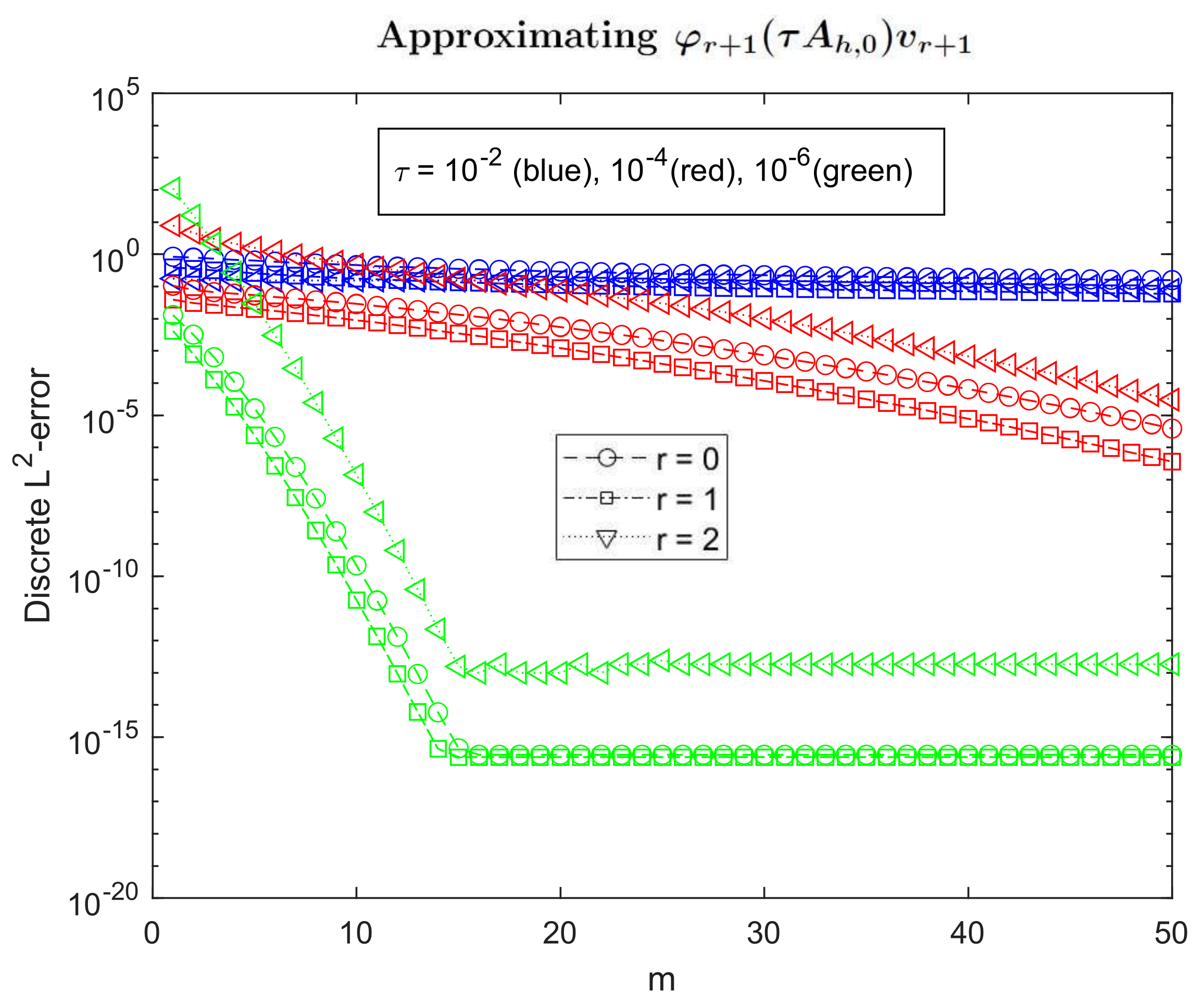
In order to see the convergence with the number of iterations for each type of terms with the standard Krylov method, in Figure 1 we represent the discrete $L^2$-error against the number of iterations when $h={10}^{-3}$ and $\tau ={10}^{-2},{10}^{-4},{10}^{-6}$. The top figure corresponds to approximating ${\phi }_j\left(\tau A_{h,0}\right)P_h\alpha$ (j = 0,1,2,3), and the bottom one to ${\phi }_j\left(\tau A_{h,0}\right)C_h\partial \alpha$ (j = 1,2,3). (We notice that, in our precise example, $\partial A^l\alpha =\pm \partial \alpha$ for any natural l). Apart from seeing that the size of errors is much bigger in the bottom plot, we can also check in both figures that the smaller $\tau$ is, the quicker the convergence with m. This corroborates the result in [3,5,6], which guarantees superlinear convergence for $m\ge \sqrt{\tau \parallel A_{h,0}\parallel }$. We would also like to remark here that Figure 1 also shows that, in spite of the fact that the convergence with m is similar, when the subindex of the function $\phi$ grows, the size of errors is smaller. Regarding the estimate of error (17), that may be due to the fact that ${\phi }_{l+1}$ evaluated at the eigenvalues of $\tau T_{m,h}$ is smaller when l grows. By looking at (14), we notice that the exponential-type functions are smaller near zero when l grows, and the convergence to zero at $-\infty$ is also a bit quicker. Look at Figure 2. Moreover, we do have the following result for the first iteration, which implies that the square of the error of the first Krylov iteration is an average of the square of the difference of $\phi$ evaluated at each eigenvalue minus its evaluation on an average of those eigenvalues:

Theorem 1.

If $\{u_1,\dots ,u_N\}$ is an orthonormal basis of eigenvectors of B, with corresponding eigenvalues $\{{\lambda }_1,\dots ,{\lambda }_N\}$, and $v={\mu }_1{u}_1+\dots +{\mu }_N{u}_N$ is a unit-norm vector, it happens that, for every analytic function defined over an interval which contains the eigenvalues,

$$\parallel \phi \left(\tau B\right)v-\phi \left(\tau t_{1,1}\right){v\parallel }^2=\sum _{k=1}^N{\mu }_k^2{[\phi \left(\tau {\lambda }_k\right)-\phi (\tau \sum _{j=1}^N{\mu }_j^2{\lambda }_j)]}^2.$$

Proof. 

On the one hand, it is clear that

$$\phi \left(\tau B\right)v={\mu }_1\phi \left(\tau {\lambda }_1\right)u_1+\dots +{\mu }_N\phi \left(\tau {\lambda }_N\right)u_N.$$

On the other hand, by Lanczos iteration, $t_{11}=v^{T}Bv$. Therefore,

$$t_{11}=\sum _{j,k=1}^N{\mu }_j{\mu }_k{u}_j^{T}B{u}_k=\sum _{j=1}^N{\mu }_j^2{\lambda }_j,$$

where the fact that $\{u_1,\dots ,u_N\}$ is an orthonormal basis of eigenvectors of B has been used in the last equality. Then,

$$\phi \left(\tau B\right)v-\phi \left(\tau t_{1,1}\right)v=\sum _{k=1}^N{\mu }_k[\phi \left(\tau {\lambda }_k\right)-\phi (\tau \sum _{j=1}^N{\mu }_j^2{\lambda }_j)]u_k,$$

from what the result follows. □

Because of this, the less $\phi$ changes in the interval where the eigenvalues of B stay, the smaller the error will be. Obviously, ${\phi }_l$ changes less in $(-\infty ,0)$ the bigger l is, which explains the relative behaviour of these functions in Figure 1.

On the other hand, in order to better understand why the errors when $v=C_h\partial \alpha$ are much bigger and, furthermore, that the smaller $\tau$ is the bigger difference with respect to the case $v=P_h\alpha$, we can consider the estimation of error (17). We notice that the fact that $\parallel v\parallel$ is much bigger for $v=C_h\partial \alpha$ than for $v=P_h\alpha$ cannot be the only reason to explain the behaviour in Figure 1 since that factor does not depend on $\tau$. Because of that, we have decided to look into the factor ${\left[{\phi }_{l+1}\left(\tau T_{m,h}\right)\right]}_{m,1}$, where $T_{m,h}$ is the tridiagonal matrix which turns up after applying Lanczos iteration to $B=A_{h,0}$. As $T_{m,h}$ is a tridiagonal symmetric matrix whose numerical range is contained in that of $B=A_{h,0}$ [31], the eigenvalues of $T_{m,h}$ are also contained in the numerical range of $A_{h,0}$, and therefore are negative and less than a value $\lambda$ for a certain $\lambda <0$. Denoting by $D_{m,h}$ the diagonal matrix containing the eigenvalues of $T_{m,h}$, it happens that

$${\phi }_{l+1}\left(\tau T_{m,h}\right)=U_{m,h}^T{\phi }_{l+1}\left(\tau D_{m,h}\right)U_{m,h},$$

for some orthogonal $(m\times m)$-matrix $U_{m,h}$, and it seems that

$${\left[{\phi }_{l+1}\left(\tau T_{m,h}\right)\right]}_{m,1}=e_m^T{U}_{m,h}^T{\phi }_{l+1}\left(\tau D_{m,h}\right)U_{m,h}{e}_1$$

is liable to behave as ${\phi }_{l+1}\left(\tau {\lambda }_{m,h}\right)$, where ${\lambda }_{m,h}$ is the biggest of eigenvalues of $T_{m,h}$. Kaniel–Paige–Saad theory [31] does not give a good bound for ${\lambda }_{m,h}$ when h is small since that bound depends on the distance to the smallest of the eigenvalues of $A_{h,0}$, which is very far from ${\lambda }_{m,h}$ for small h. We notice that, for $m=1$, ${\lambda }_{1,h}(C_h\partial \alpha )\approx -2\times {10}^6$ while ${\lambda }_{1,h}\left(P_h\alpha \right)\approx -2\times {10}^3$. Because of that, the quotient of the estimation of errors (17) when applying Krylov standard method with $m=1$, $v=C_h\partial \alpha$ and $v=P_h\alpha$ is approximately

$$\begin{array}{ccc}& & \parallel C_h\partial \alpha \parallel \frac{{\phi }_{l+1}(-2\times {10}^4)t_{21}(C_h\partial \alpha )}{{\phi }_{l+1}(-2\times 10)t_{21}\left(P_h\alpha \right)},\tau ={10}^{-2},\hfill \\ & & \parallel C_h\partial \alpha \parallel \frac{{\phi }_{l+1}(-200)t_{21}(C_h\partial \alpha )}{{\phi }_{l+1}(-0.2)t_{21}\left(P_h\alpha \right)},\tau ={10}^{-4},\hfill \\ & & \parallel C_h\partial \alpha \parallel \frac{{\phi }_{l+1}(-2)t_{21}(C_h\partial \alpha )}{{\phi }_{l+1}(-2\times {10}^{-3})t_{21}\left(P_h\alpha \right)},\tau ={10}^{-6}.\hfill \end{array}$$

The behaviour of the functions ${\phi }_{l+1}$, as plotted in Figure 2, explains that this factor increases from the top to the bottom, i.e., when $\tau$ decreases.

In order to understand what happens when m increases, we have observed that $t_{m+1,m}(C_h\partial \alpha )/t_{m+1,m}\left(P_h\alpha \right)$ is constant for $m\ge 2$. Moreover, we represent ${\lambda }_{m,h}\left(P_h\alpha \right)$ and ${\lambda }_{m,h}(C_h\partial \alpha )$ in Figure 3. They both seem to converge to the same quantity but, in any case, for the values of $m=1,\dots ,50$ (which are considered in Figure 1), ${\lambda }_{m,h}(C_h\partial \alpha )/{\lambda }_{m,h}\left(P_h\alpha \right)$ is still very big, which explains the different relative behaviour of both plots in Figure 1 also for $m=2,\dots ,50$.

As for the behaviour when h gets smaller, although not shown here for the sake of brevity, it is already well-known that the standard Krylov iteration does not give uniform convergence and, the smaller h is, the bigger m must be to get a given error for the approximation [6,14].

What subroutine phipm.m does in order to calculate (6) is not to apply Krylov iteration to each of the terms in that expression. The more natural seems to choose $b_j$ in (11) as

$$b_0=P_h\alpha ,b_{l+1}=C_h\partial A^l\alpha ,l=0,\dots ,r,$$

and the corresponding time-stepping (15) and (16) is performed, where Krylov iteration is just applied to approximate ${\phi }_{r+1}\left(s_k{B}_0\right)w_{r+1}$. Doing things that way, Table 1 is obtained. On the one hand, the fact that just the biggest ${\phi }_{r+1}$ is considered in (6) for Krylov iteration is positive, since the errors are smaller when r grows. On the other hand, from what can be observed at least for $tol={10}^{-7}$, the bigger errors coming from the consideration of the terms on $C_h\partial \alpha$ seem to be ameliorated by the factors $s_k^l$ in (16), since the more terms of that type are considered, the less CPU time the subroutine requires to get a given accuracy.

3.3. Suggestion to Improve the Result with Phipm.m

In order to simplify time-stepping, what we suggest in this section is to apply recurrence (14) to (6) and (7) before attempting to use subroutine phipm.m. More precisely, we take profit of the following result.

Proposition 1.

For $r\ge 0$, formulas (6) and (7) can be written, respectively, as

$$\begin{array}{c}{\displaystyle P_h\alpha +\sum _{j=1}^r\frac{{\tau }^j}{j!}[A_{h,0}^j{P}_h\alpha +\sum _{l=0}^{j-1}{A}_{h,0}^l{C}_h\partial A^{j-l-1}\alpha ]}\end{array}$$

$$\begin{array}{c} +{\tau }^{r+1}{\phi }_{r+1}\left(\tau A_{h,0}\right)[A_{h,0}^{r+1}{P}_h\alpha +\sum _{l=0}^r{A}_{h,0}^l{C}_h\partial A^{r-l}\alpha ],\\ P_h\alpha +{\displaystyle \sum _{i=1}^r}\frac{{\tau }^{j+i}}{(j+i)!}[A_{h,0}^i{P}_h\alpha +{\displaystyle \sum _{l=0}^{i-1}}{A}_{h,0}^l{C}_h\partial A^{i-l-1}\alpha ]\end{array}$$

(19)

$$\begin{array}{ccc}& & +{\tau }^{r+1}{\phi }_{j+r+1}\left(\tau A_{h,0}\right)[A_{h,0}^{r+1}{P}_h\alpha +\sum _{l=0}^r{A}_{h,0}^l{C}_h\partial A^{r-l}\alpha ].\hfill \end{array}$$

(20)

Proof. 

The proof follows by induction on r. Notice that, for $r=0$ and formula (6), using the first formula of (14) with $j=0$,

$$\begin{array}{ccc}\hfill e^{\tau A_{h,0}}{P}_h\alpha +\tau {\phi }_1\left(\tau A_{h,0}\right)C_h\partial \alpha & =& [\tau A_{h,0}{\phi }_1\left(\tau A_{h,0}\right)+I]P_h\alpha +\tau {\phi }_1\left(\tau A_{h,0}\right)C_h\partial \alpha \hfill \\ & =& P_h\alpha +\tau {\phi }_1\left(\tau A_{h,0}\right)[A_{h,0}{P}_h\alpha +C_h\partial \alpha ].\hfill \end{array}$$

Then, assuming that (19) is the same as (6), the same equivalence is true for $r+1$, since

$$\begin{array}{c}{\displaystyle e^{\tau A_{h,0}}{P}_h\alpha +\sum _{l=0}^{r+1}{\tau }^{l+1}{\phi }_{l+1}\left(\tau A_{h,0}\right)C_h\partial A^l\alpha }\hfill \\ =P_h\alpha +{\displaystyle \sum _{j=1}^r}\frac{{\tau }^j}{j!}\left[A_{h,0}^j{P}_h\alpha +{\displaystyle \sum _{l=0}^{j-1}}{A}_{h,0}^l{C}_h\partial A^{j-l-1}\alpha \right]\hfill \\ +{\tau }^{r+1}{\phi }_{r+1}\left(\tau A_{h,0}\right)\left[A_{h,0}^{r+1}{P}_h\alpha +{\displaystyle \sum _{l=0}^r}{A}_{h,0}^l{C}_h\partial A^{r-l}\alpha \right]\hfill \\ +{\tau }^{r+2}{\phi }_{r+2}\left(\tau A_{h,0}\right)C_h\partial A^{r+1}\alpha \hfill \\ =P_h\alpha +{\displaystyle \sum _{j=1}^{r+1}}\frac{{\tau }^j}{j!}\left[A_{h,0}^j{P}_h\alpha +{\displaystyle \sum _{l=0}^{j-1}}{A}_{h,0}^l{C}_h\partial A^{j-l-1}\alpha \right]\hfill \\ +{\tau }^{r+2}{\phi }_{r+2}\left(\tau A_{h,0}\right)\left[A_{h,0}^{r+2}{P}_h\alpha +{\displaystyle \sum _{l=0}^r}{A}_{h,0}^{l+1}{C}_h\partial A^{r-l}\alpha +C_h\partial A^{r+1}\alpha \right],\hfill \end{array}$$

where, for the second equality, ${\phi }_{r+1}$ has been substituted from its expression when solving from the first formula in (14) with $j=r+1$. It is then easy to see that this expression is equivalent to (19) with r changed by $r+1$.

The proof follows in a similar way for (20). □

Let us now concentrate on (19). Calling subroutine phipm.m just for the last term of this expression, i.e., taking

$$\begin{array}{c}\hfill b_j=0,j=0,\dots ,r,b_{r+1}=A_{h,0}^{r+1}{P}_h\alpha +\sum _{l=0}^r{A}_{h,0}^l{C}_h\partial A^{r-l}\alpha ,\end{array}$$

(21)

many calculations in the time-stepping procedure (15) and (16) are avoided and, in some way, calculated just once and for all at the beginning in expression (19). We also notice that each bracket in this expression is approximating $A^j\alpha$ ($j=1,\dots ,r+1$) when $h\to 0$, with the only remark that, the bigger j is, the more relevant the errors coming from the ill-posedness of numerical differentiation in space may be. Nevertheless, for smaller values of j, those brackets are controlled and, under enough regularity of $\alpha$, do not grow in norm for the values of h, which are usually required for enough accuracy in space. Another important remark is that each of those brackets can be recursively calculated from the previous one just by multiplying by $A_{h,0}$ and summing a term like $C_h\partial A^l\alpha$. Therefore, many fewer calculations than those apparent are really necessary.

The results doing things that way for the example in Section 2.1 are shown in

Table 2. CPU time to calculate (6) for the data in Section 2.1 using formula (19) and subroutine phipm.m just for the last term.

	$\mathit{r}=0$	$\mathit{r}=1$	$\mathit{r}=2$
$tol={10}^{-7}$	4.9e-01	4.2e-01	3.9e-01
$tol={10}^{-13}$	8.1e-01	6.5e-01	5.8e-01

, where the improvement with respect to the results on cpu time in Table 1 are evident. Moreover, for the smallest tolerance, not only the necessary time to achieve a similar error (related to $tol={10}^{-13}$) is smaller, but we also notice that increasing the value of r, that time is smaller (as it also happened with $tol={10}^{-7}$ in Table 1). This seems to suggest that rounding errors due to time-stepping in Table 1 were too important.

In order to better understand why taking bigger r implies that CPU time is smaller, we have applied Krylov iteration to

$${\phi }_{r+1}\left(\tau A_{h,0}\right)v_{r+1},r=0,1,2,$$

where

$$\begin{array}{ccc}\hfill v_1& =& A_{h,0}{P}_h\alpha +C_h\partial \alpha ,\hfill \\ \hfill v_2& =& A_{h,0}{v}_1+C_h\partial A\alpha ,\hfill \\ \hfill v_3& =& A_{h,0}{v}_2+C_h\partial A^2\alpha .\hfill \end{array}$$

(22)

Notice that ${\phi }_{r+1}\left(\tau A_{h,0}\right)v_{r+1}$ is the last term in (19) except for the factor ${\tau }^{r+1}$ and that, in exact arithmetic, when $h\to 0$,

$$v_{r+1}\approx A^{r+1}\alpha ,r=0,1,2.$$

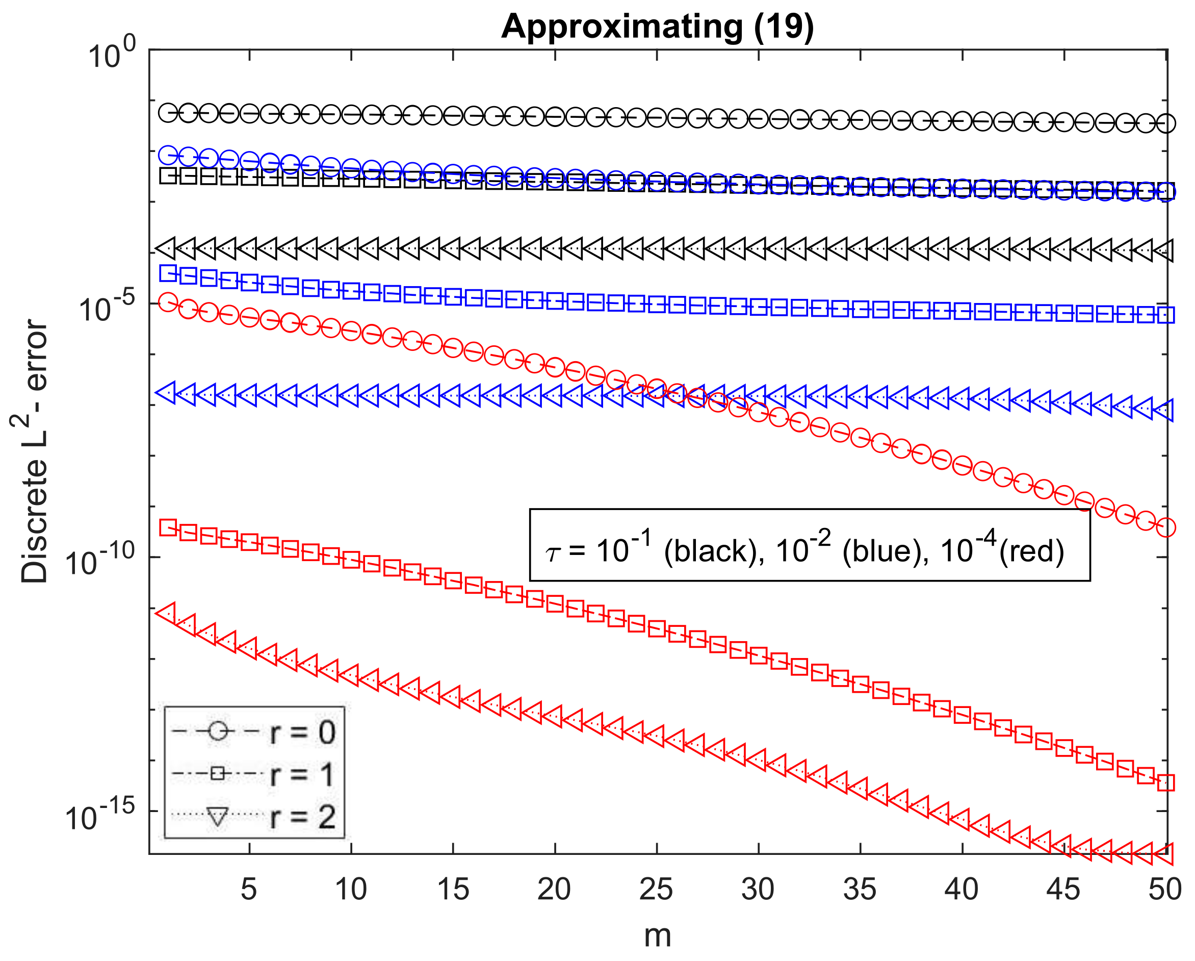
In Figure 4, we again represent the $L^2$-discrete error against the number of Krylov iterations for different values of $\tau ={10}^{-2},{10}^{-4},{10}^{-6}$. We can again see that the smaller $\tau$ is, the quicker the convergence with m. As for the size of errors, for $r=0,1$, they are quite similar to the first plot in Figure 1, and therefore not as big as in the second plot of the same figure. However, for $r=2$, the errors are quite bigger than the corresponding ones in that first plot and, in any case, bigger than those of $r=0,1$. This is due to the fact that $\parallel v_3\parallel$ can be numerically seen to be of order ${10}^5$ in spite of the fact of being presumable approximating $A^3\alpha =-\alpha$. This is caused by roundoff errors, since numerical differentiation is a badly posed problem and a sixth-order space derivative is being considered.

On the other hand, the other terms in (19) are exactly calculated except for roundoff. Therefore, the error when calculating the whole expression should be the error which was represented in Figure 4 multiplied by ${\tau }^{r+1}$. This explains that, in Figure 5, the errors are so small even for $\tau ={10}^{-1},{10}^{-2},{10}^{-4}$. Moreover, the error is smaller when r increases, not only from $r=0$ to $r=1$, but also from $r=1$ to $r=2$ (although in a smaller proportion). This is the reason why taking a bigger value of r can decrease the computational cost when using phipm.m to approximate (6).

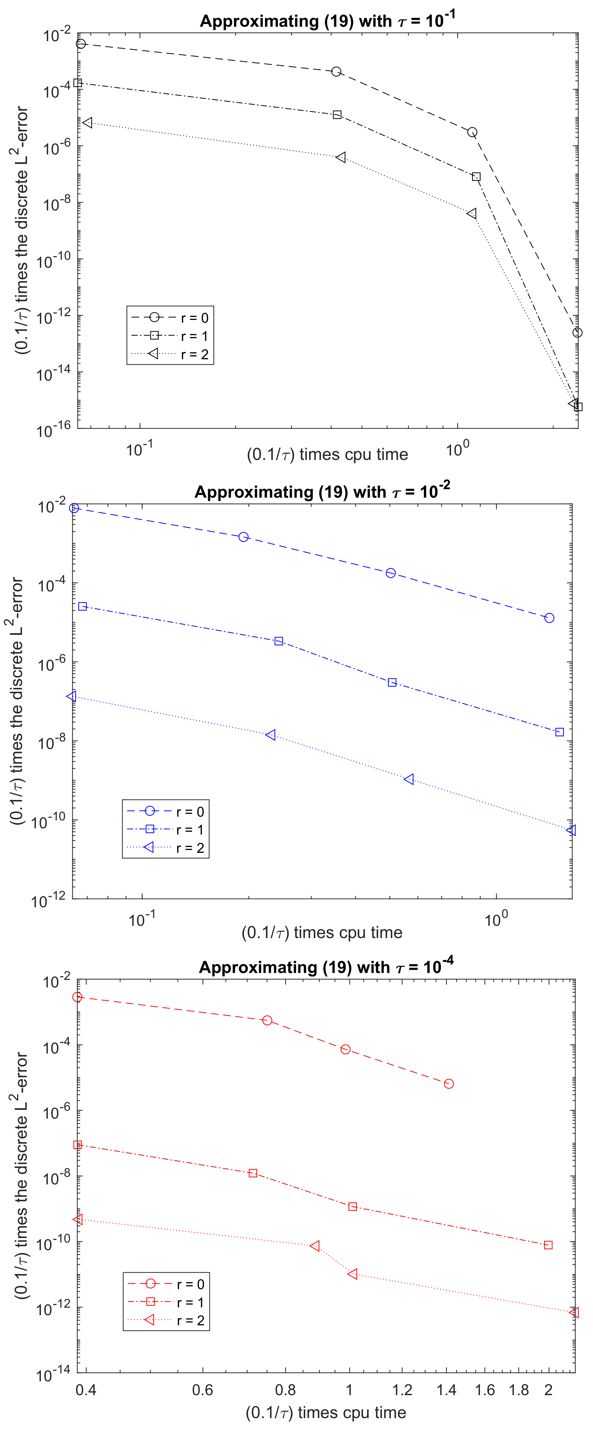
To better illustrate that when trying to approximate (6) with $\tilde{\tau }=0.1$, we represent in Figure 6 $(0.1/\tau )$ times the error when approximating (6) through (19) against $(0.1/\tau )$ times the CPU required to calculate (6) for $\tau =0.1,{10}^{-2},{10}^{-4}$ and different values of m. In such a way, we are implicitly assuming that, in order to approximate (6) with $\tilde{\tau }=0.1$,

• exact $(0.1/\tau )$ steps are made through time-stepping in the Krylov iteration in (19);
• the cost of the first part in (19) is negligible;
• the errors committed at each step sum linearly.

These assumptions are not completely satisfied but, in such a way, we can have an overview of the total cost to calculate (19) for the different values of r. As Figure 6 shows, $r=2$ seems cheaper than $r=1$ and this one cheaper than $r=0$.

Although not shown here for the sake of brevity, similar arguments apply for the case in which (7) is to be approximated with the same subroutine.

3.4. Modification of Subroutine Phipm.m

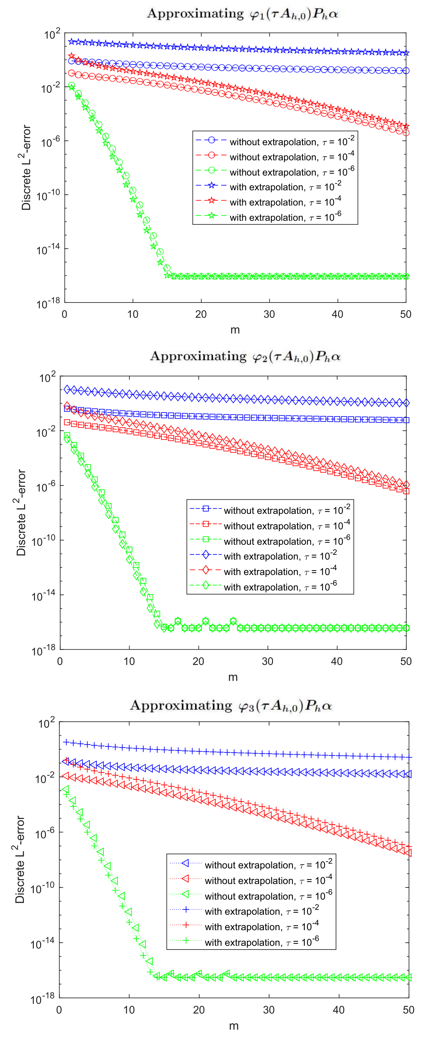
Estimate (17) was originally proposed in [9] in a context where it was reasonable just when $\parallel \tau B\parallel <1$. For our purposes, and as it was also stated in [7], that is not useful. In fact, in Figure 7, we represent the discrete $L^2$-error against the number of Krylov iterations when approximating ${\phi }_{r+1}\left(\tau A_{h,0}\right)P_h\alpha$ using the extrapolation (18) and when not using it (8). We can see that, only when $\tau$ is very small so that $\parallel \tau A_{h,0}\parallel$ is near 1, the extrapolation formula improves the standard one. However, in [7], by relating it to the error which is committed when integrating linear systems with the standard Krylov method, the following similar estimate was obtained:

$$\begin{array}{c}\hfill {\tilde{\epsilon }}_m=\parallel v\parallel \tau t_{m+1,m}{\left[{\phi }_l\left(\tau T_m\right)\right]}_{m,1}{v}_{m+1},\end{array}$$

(23)

where the difference comes from the subindex in the $\phi$-function evaluated at $T_m$, which is now l instead of $l+1$. Notice that, in such a case, the augmented matrix of size $m+l+1$ does not need to be calculated, and it is enough to consider that in (9), which just has dimension $m+l$. As the authors mention in [7], (23) is not the first term of a series for the whole error, but it is just a rough estimate. Therefore, extrapolation has no sense in this case. If we change subroutine phipm.m accordingly, without considering the extrapolation (18) but just (8), and leaving the same adaptive strategy but with the new error estimation (23), the results in

Table 3. CPU time to calculate (6) for the data in Section 2.1 using formula (19) and a modification of subroutine phipm.m (with error estimate (23) and without extrapolation) just for the last term.

	$\mathit{r}=0$	$\mathit{r}=1$	$\mathit{r}=2$
$tol={10}^{-7}$	3.9e-01	3.4e-01	3.5e-01
$tol={10}^{-13}$	1.0e+00	5.9e-01	5.3e-01

are obtained when approximating (6), where again expression (19) and the choice (21) are used.

In this table, we can see that the CPU time which is required to achieve a given tolerance is smaller than in Table 2 for $tol={10}^{-7}$. This agrees with the fact that, when the stepsize is not very small, not doing extrapolation is more accurate and cheap than doing it. For the smaller tolerance $tol={10}^{-13}$, the CPU time which is required when $r=0$ is a bit bigger than in Table 2, which may be due to the fact that, in this particular case, the stepsizes which the subroutine has to take are so small that the extrapolation is worth doing. In any case, CPU time continues to diminish from $r=0$ to $r=1$ for both tolerances and, in the same way than in Table 2, it diminishes also for $tol={10}^{-13}$ from $r=1$ to $r=2$.

4. Purely Rational Krylov Method

Exponential methods are in principle constructed so that linear systems do not have to be solved when integrating stiff linear problems with standard implicit methods. For non-linear stiff problems, standard Rosenbrock methods are usually used, which avoid to solve a non-linear problem at each stage by the use of the Jacobian of the problem. In any case, the calculation of this Jacobian at each step can be difficult or expensive and, therefore, this part may be more costly than the one of having to solve a linear system at each stage. Because of this, extended Krylov methods which require the calculation of powers of the inverse of a certain sparse matrix applied over a vector are justified when applied inside exponential methods which aim to solve non-linear problems. More precisely, although the calculations of those terms imply solving linear systems with sparse matrices, its cost may be justified in non-linear problems because the Jacobian of the non-linear function does not need to be calculated. We notice that, if Gaussian elimination for sparse matrices is used, as the matrix is always the same, the LU factorization is done once and for all at the very beginning. Moreover, if multigrid methods are used, the computational cost is just of the order of the number of grid points in the space discretization (the same order of the number of computations which are required when multiplying a sparse matrix times a vector in standard Krylov methods).

Extended Krylov subspace methods for symmetric matrices were described in [11] and estimates of convergence where given in terms of the smallest and biggest of the eigenvalues. In such a way, similarly to standard Krylov methods, they are not uniform convergence estimates on the spacegrid when the matrices come from the discretization of an unbounded operator but, as distinct, those estimates were smaller than those of standard Krylov methods and, in practice, the true error was even much smaller than those estimates. Much better estimates of the error observed in practice were obtained in [16] for both symmetric and nonsymmetric B, although just for the case in which the corresponding Krylov space contains the same number of positive and negative powers of B and for matrix functions, which do not include the exponential-type functions in which we are interested.

In this paper, we will centre on the purely rational Krylov method, which is based on considering as Krylov subspace

$$\begin{array}{c}\hfill <v,{(\gamma I-B)}^{-1}v,\dots ,{(\gamma I-B)}^{-m+1}v>,\end{array}$$

(24)

for a certain real parameter $\gamma$ for which the inverse of $\gamma I-B$ exists. An analysis of this method is performed in [14] when the matrix B is substituted by an unbounded operator with a field of values on the left half plane. In such a way, estimates of the error are obtained which are valid for discretizations of such an operator which are independent of the grid size. Furthermore, the bounds of the error which are proved in [14] are smaller when the index of the function ${\phi }_l$ grows. More precisely, they decrease like

$$\begin{array}{c}\hfill O(\parallel v\parallel m^{-\frac{l}{2}}),\end{array}$$

(25)

although in practice, an exponential decay can be observed.

Using both powers of B and ${(\gamma I-B)}^{-1}$ has been proven to be advantageous when some powers $B^{l}v$ are bounded. More precisely, in the case that v discretizes a function which vanishes at the boundary and which satisfies that several of the powers of A exist and also vanish at the same boundary, in [13] it is shown that the rate of convergence is quicker ($O(\parallel B^{q}v\parallel m^{-\frac{l+q}{2}})$ if $B^{l}v$ is bounded for $0\le l\le q$) when, in the Krylov subspace, those powers of B are considered as well as those on ${(\gamma I-B)}^{-1}$. Numerically, even a higher order rate of convergence can be observed, which approximates that of the purely rational Krylov method.

In any case, as we are just interested in problems with non-vanishing boundary conditions, we will directly consider the purely rational Krylov method, which is based on constructing iteratively an orthonormal basis of the Krylov subspace (24) through Lanczos iteration.

If we denote by $V_m$ also to the matrix whose columns are that orthonormal basis, the projection onto that space (24) is given by $Q_m=V_m{V}_m^H$. The approximation to ${\phi }_l\left(\tau B\right)v$ is then given by ${\phi }_l\left(\tau B_m\right)v$, where $B_m=Q_{m}B{Q}_m$. Therefore,

$$\begin{array}{ccc}\hfill {\phi }_l\left(\tau B\right)v& \approx & {\phi }_l\left(\tau B_m\right)v={\phi }_l\left(\tau Q_{m}B{Q}_m\right)v={\phi }_l\left(\tau V_m{V}_m^{H}B{V}_m{V}_m^H\right)v\hfill \\ & =& V_m{\phi }_l\left(\tau V_m^{H}B{V}_m\right)V_m^{H}v=\parallel v\parallel V_m{\phi }_l\left(\tau S_m\right)e_1,\hfill \end{array}$$

where

$$S_m=\left[\begin{array}{ccc}<B{v}_1,v_1>& \dots & <B{v}_m,v_1>\\ ⋮& \ddots & ⋮\\ <B{v}_1,v_m>& \dots & <B{v}_m,v_m>\end{array}\right],$$

and ${\phi }_l\left(\tau S_m\right)e_1$ is calculated through $expm\left(\tau {\widehat{S}}_m\right)$, where ${\widehat{S}}_m$ is like ${\widehat{T}}_m$ in (9) with $T_m$ substituted by $S_m$.

Application to Our Problem

The aim of this section is to apply the purely rational Krylov method just described to our problem in Section 2.1.

In a similar way to Figure 1 and Figure 4 in Section 3.2 for the standard Krylov method, in Figure 8 we represent, for $r=0,1,2$, the error when approximating ${\phi }_{r+1}\left(\tau A_{h,0}\right)P_h\alpha$, ${\phi }_{r+1}\left(\tau A_{h,0}\right)C_h\partial A^r\alpha$ and ${\phi }_{r+1}\left(\tau A_{h,0}\right)v_{r+1}$ with $v_{r+1}$ in (22) against the number of iterations. We have taken now $\tau ={10}^{-1},{10}^{-2},{10}^{-3}$ and, as distinct as what happened with the standard Krylov method and not explained in the literature, the convergence with m is now quicker when $\tau$ is bigger and, in any case, exponential from the very beginning ($m=1$) although with a smaller rate when $\tau$ diminishes. Because of this, time-stepping has no sense with this method and the best approach is to apply Krylov iteration directly with the value of $\tau$ in which we are interested in (6).

As for the behaviour for the different values of the index l in ${\phi }_l$, in the same way as with standard Krylov iteration, the errors are smaller when l grows. We notice that, for $m=1$, this method coincides with standard Krylov iteration and therefore, the explanation for that is given in Theorem 1. On the other hand, the rate of convergence also seems to be more advantageous when l grows, as in accordance with bound (25).

Although not shown here for the sake of brevity, we have also run our experiments with smaller values of the grid size h and we have seen that the errors are very similar. This agrees with the analysis performed for rational Krylov methods in [14], and this behaviour makes this method more interesting than the standard one, which does not show uniform convergence on the space grid size. (Only when calculating ${\phi }_3\left(\tau A_{h,0}\right)v_3$, the errors are a bit bigger when h diminishes for the higher values of m, and that is due to the fact that the calculation of $v_3$ is already quite difficult when h is small).

In any case, what is important is the behaviour of the error when approximating (19) against the number of iterations m for the different values of $r=0,1,2$.

That can be observed in Figure 9. We notice that the error now is that of the bottom graph of Figure 8 multiplied by ${\tau }^{r+1}$. We restrict here to the case $\tau =0.1$, since the aim is to approximate (6) with that value of $\tau$. What we can observe in (Figure 8) is that the error is smaller with $r=1$ than with $r=0$, and also slightly smaller with $r=2$ than with $r=1$.

5. General Conclusions

• At least for the range of values in which we move in the example of Section 2.1, calculating (6) or (7) with a given required accuracy is likely to be cheaper when r increases, in spite of the fact that, apparently, more terms need to be calculated.
• In the case that having to solve several linear systems at each step with a same matrix is not a drawback for having chosen an exponential method to integrate a problem like (1), we recommend to approximate (6) or (7) by using (19) or (20) and a purely rational Krylov method to calculate the last term there.
• Whenever having to solve several linear systems at each step is a drawback for using exponential methods to integrate a problem like (1), we recommend using the modification of the adaptive subroutine phipm.m, which is described in Section 3.4, although the subroutine phipm.m applied as described in Section 3.3 also gives quite acceptable results, at least in our precise example.

References

- Moler, C.; Loan, C.V. Nineteen dubious ways to compute the exponential of a matrix. SIAM Rev. 1978, 20, 801–836. [Google Scholar] [CrossRef]
- Moler, C.; Loan, C.V. Nineteen dubious ways to compute the exponential of a matrix, twenty-five years later. SIAM Rev. 2003, 45, 3–49. [Google Scholar] [CrossRef]
- Druskin, V.L.; Knizhnerman, L.A. Two polynomial methods of calculating functions of symmetric matrices. USSR Comput. Math. Math. Phys. 1989, 29, 112–121. [Google Scholar] [CrossRef]
- Druskin, V.L.; Knizhnerman, L.A. Error bounds in the simple Lanczos procedure for computing functions of symmetric matrices and eigenvalues. Comput. Maths. Math. Phys. 1991, 31, 970–983. [Google Scholar]
- Druskin, V.L.; Knizhnerman, L.A. Krylov subspace approximations of eigenpairs and matrix functions in exact and computer arithmetic. Numer. Linear Algebra Appl. 1995, 2, 205–217. [Google Scholar] [CrossRef]
- Hochbruck, M.; Lubich, C. On Krylov subspace approximations to the matrix exponential operator. SIAM J. Numer. Anal. 1997, 34, 1911–1925. [Google Scholar] [CrossRef]
- Hochbruck, M.; Lubich, C.; Selhofer, H. Exponential Integrators for Large Systems of Differential Equations. SIAM J. Sci. Comput. 1998, 19, 1552–1574. [Google Scholar] [CrossRef] [Green Version]
- Niesen, J.; Wright, W.M. Algorithm 919: A Krylov subspace algorithm for evaluating the φ-functions appearing in exponential integrators. ACM Trans. Math. Softw. 2012, 38, 22. [Google Scholar] [CrossRef] [Green Version]
- Saad, Y. Analysis of some Krylov subspace approximations to the matrix exponential operator. SIAM J. Numer. Anal. 1992, 29, 209–228. [Google Scholar] [CrossRef]
- Sidje, R.B. EXPOKIT: A Software Package for Computing Matrix Exponentials. ACM Trans. Math. Softw. 1998, 24, 130–156. [Google Scholar] [CrossRef]
- Druskin, V.L.; Knizhnerman, L.A. Extended Krylov subspaces: Approximation of the square root and related functions. SIAM J. Matrix Anal. Appl. 1998, 19, 755–771. [Google Scholar] [CrossRef]
- Eshof, J.V.D.; Hochbruck, M. Preconditioning Lanczos approximations to the matrix exponential. SIAM J. Sci. Comput. 2006, 27, 1438–1457. [Google Scholar] [CrossRef] [Green Version]
- Göckler, T.; Grimm, V. Convergence analysis of an extended Krylov subspace method for the approximation of operator functions in exponential integrators. SIAM J. Numer. Anal. 2013, 51, 2189–2213. [Google Scholar] [CrossRef] [Green Version]
- Grimm, V. Resolvent Krylov subspace approximation to operator functions. BIT Numer. Math. 2012, 52, 639–659. [Google Scholar] [CrossRef]
- Jagels, C.; Reichel, L. The extended Krylov subspace method and orthogonal Laurent polynomials. Linear Algebra Its Appl. 2009, 431, 441–458. [Google Scholar] [CrossRef] [Green Version]
- Knizherman, L.; Simoncini, V. A new investigation of the extended Krylov subspace method for matrix function evaluations. Numer. Linear Algebra Appl. 2010, 17, 615–638. [Google Scholar]
- López, L.; Simoncini, V. Analysis of projection methods for rational function approximation to the matrix exponential. SIAM J. Num. Anal. 2006, 44, 613–635. [Google Scholar] [CrossRef] [Green Version]
- Moret, I.; Novati, P. RD-Rational approximations of the matrix exponential. BIT Numer. Math. 2004, 44, 595–615. [Google Scholar] [CrossRef]
- Hochbruck, M.; Ostermann, A. Exponential integrators. Acta Numer. 2010, 29, 209–286. [Google Scholar] [CrossRef] [Green Version]
- Alonso-Mallo, I.; Cano, B.; Reguera, N. Analysis of order reduction when integrating linear initial boundary value problems with Lawson methods. Appl. Numer. Math. 2017, 118, 64–74. [Google Scholar] [CrossRef] [Green Version]
- Cano, B.; Reguera, N. Order reduction and how to avoid it when Lawson methods integrate reaction-diffusion boundary value problems. arXiv 2019, arXiv:1909.12659. [Google Scholar]
- Faou, E.; Ostermann, A.; Schratz, K. Analysis of exponential splitting methods for inhomogeneous parabolic equations. IMA J. Numer. Anal. 2015, 35, 161–178. [Google Scholar] [CrossRef]
- Hochbruck, M.; Ostermann, A. Explicit exponential Runge-Kutta methods for semilinear parabolic problems. SIAM J. Num. Anal. 2005, 43, 1069–1090. [Google Scholar] [CrossRef] [Green Version]
- Alonso-Mallo, I.; Cano, B.; Reguera, N. Avoiding order reduction when integrating linear initial boundary value problems with Lawson methods. IMA J. Numer. Anal. 2017, 37, 2091–2119. [Google Scholar] [CrossRef] [Green Version]
- Alonso-Mallo, I.; Cano, B.; Reguera, N. Avoiding order reduction when integrating linear initial boundary value problems with exponential splitting methods. IMA J. Numer. Anal. 2018, 38, 1294–1323. [Google Scholar] [CrossRef]
- Alonso-Mallo, I.; Cano, B.; Reguera, N. Avoiding order reduction when integrating reaction-diffusion boundary value problems with exponential splitting methods. J. Comput. Appl. Math. 2019, 357, 228–250. [Google Scholar] [CrossRef] [Green Version]
- Cano, B.; Moreta, M.J. Exponential quadrature rules without order reduction for integrating linear initial boundary value problems. SIAM J. Num. Anal. 2018, 56, 1187–1209. [Google Scholar] [CrossRef]
- Cano, B.; Moreta, M.J. How to Avoid Order Reduction When Explicit Runge-Kutta Exponential Methods Integrate Nonlinear Initial Boundary Value Problems; Submitted for Publication.
- Cano, B.; Reguera, N. Avoiding order reduction when integrating nonlinear Schrödinger equation with Strang method. J. Comp. Appl. Math. 2017, 316, 86–99. [Google Scholar] [CrossRef] [Green Version]
- Cano, B.; Reguera, N. How to Avoid Order Reduction When Lawson Methods Integrate Nonlinear Initial Boundary Value Problems. Submitted for Publication.
- Golub, G.H.; van Loan, C.F. Matrix Computations, 4th ed.; The Johns Hopkins University Press: Baltimore, MD, USA, 2013. [Google Scholar]
- Higham, N.J. The scaling and squaring method for the matrix exponential revisited. SIAM J. Matrix Anal. Appl. 2005, 26, 1179–1193. [Google Scholar] [CrossRef]
- Skaflestad, B.; Wright, W. The scaling and modified squaring method for matrix functions related to the exponential. Appl. Numer. Math. 2009, 59, 783–799. [Google Scholar] [CrossRef]
Figure 1.
Discrete -error against number of Krylov iterations when approximating (top) and (bottom) through standard Krylov method for different values of , and fixed .
Figure 2.
(continuous line), (dashed line), (dash-dotted line), (dotted line).
Figure 3.
against number of iterations for and both , .
Figure 4.
Discrete -error against number of Krylov iterations when approximating for in (22), different values of , and fixed .
Figure 5.
Discrete -error against number of Krylov iterations when approximating (19) for the data in Section 2.1 for different values of , and fixed .
Figure 6.
times the discrete -error against times CPU time when approximating (19) for the data in Section 2.1 for (), () and (), and fixed .
Figure 7.
Discrete -error against number of Krylov iterations when approximating for the data in Section 2.1 for different values of with extrapolation (18) and without it, (top), (middle), (bottom), ().
Figure 8.
Discrete -error against number of Krylov iterations when approximating , , for the data in Section 2.1 through purely rational Krylov methods for different values of , , and fixed .
Figure 9.
Discrete -error against number of Krylov iterations when approximating (6) for the data in Section 2.1 through (19) using purely rational Krylov method for , and fixed