
A Fast and Effective Method to Identify Relevant Sets of Variables in Complex Systems


1
Department of Physics, Informatics and Mathematics, University of Modena and Reggio Emilia, 41121 Modena, Italy
2
Institute for Advanced Studies, University of Amsterdam, 1012 WX Amsterdam, The Netherlands
3
European Centre for Living Technology, 30123 Venice, Italy
*
Author to whom correspondence should be addressed.
Mathematics 2021, 9(9), 1022; https://0-doi-org.brum.beds.ac.uk/10.3390/math9091022
Submission received: 17 February 2021
/
Revised: 19 April 2021
/
Accepted: 27 April 2021
/
Published: 30 April 2021
(This article belongs to the Special Issue Computational Approaches for Data Inspection in Biomedicine)
Abstract
:In many complex systems one observes the formation of medium-level structures, whose detection could allow a high-level description of the dynamical organization of the system itself, and thus to its better understanding. We have developed in the past a powerful method to achieve this goal, which however requires a heavy computational cost in several real-world cases. In this work we introduce a modified version of our approach, which reduces the computational burden. The design of the new algorithm allowed the realization of an original suite of methods able to work simultaneously at the micro level (that of the binary relationships of the single variables) and at meso level (the identification of dynamically relevant groups). We apply this suite to a particularly relevant case, in which we look for the dynamic organization of a gene regulatory network when it is subject to knock-outs. The approach combines information theory, graph analysis, and an iterated sieving algorithm in order to describe rather complex situations. Its application allowed to derive some general observations on the dynamical organization of gene regulatory networks, and to observe interesting characteristics in an experimental case.
1. Introduction
The available molecular data suggests the existence of a vast number of pathways, networks of interactions, and chemical environments. A large quantity of information is available on many biological systems, and researchers use it to infer global properties of biological networks [1,2,3,4,5,6]. There are, however, major limitations which affect most studies in the field, the most relevant being that (i) the information about the underlying true interactions is often incomplete and that (ii) many studies rely on “static” topological information. However, in order to understand the functionality of a system, it is important to study its dynamical properties and it is therefore worthwhile to resort to methods able to detect and provide information about the dynamical organization of the system under examination.
In complex systems, even if the elements and their interactions are reasonably well-known (so that one has a good knowledge at the “microscopic” level) it is very often not easy (or even not possible) to deduce the overall behaviors from this microscopic knowledge. Moreover, the emergence of intermediate structures is frequently observed, which must be taken into account to provide a meaningful description of the overall properties of the system. Examples of intermediate levels abound in biology, including organs, which are necessary to describe a multicellular organism (the macrolevel) composed by several cells (the microlevel). In turn, organelles can be regarded as intermediate entities between macromolecules and cells, tissues between cells and organs, etc.
While different sciences have developed their own heuristics and strategies to cope with the presence of these intermediate levels [7,8,9,10,11,12], it is advisable to develop general methods applicable to several different areas. We have proposed one such method, whose specific aim is that of identifying subsets of system variables that (i) are well coordinated among themselves and (ii) have a weaker interaction with the remainder of the system. They have been called Relevant Sets (or shortly RSs in the following), since their identification can often lead to a high-level description of the organization the system, and thus to a better understanding of its properties [13].
In order to identify the Relevant Sets, we have developed the Relevance Index (RI) method [13,14,15], which is used to evaluate, for each subset of variables, how well they satisfy conditions (i) and (ii) above. Inspired by work by Tononi and Edelman [8,16,17], it makes use of some information-theoretical measures, which can be computed from the observations of the values of the system variables in different circumstances (which often, but not necessarily, correspond to different observation times) [15,18,19,20]. By directly applying the RI method to various subsets and by ranking them according to their RI evaluations, one finds overlapping sets with similar values of the index, a condition which makes it very difficult to identify what the RSs really are. In order to avoid this pitfall, we also introduced an “iterative sieving” algorithm which leads to the identification of disjoint RSs, which can in turn be combined to obtain larger relevant sets. The method has been widely described in the literature [13,15,21] and is briefly summarized in Section 2 below. For the sake of clarity, it will be called the “full RI method” in this paper.
We have applied our method to some artificial models, in order to test its capability to actually detect RSs, and to some interesting cases from natural and also social sciences, including the interpretation of metabolic pathways [22] and of autocatalytic systems in chemistry [14,15], the identification of communities in socio-economic systems [13,23], the detection of specific groups of genes ruling the dynamics of genetic networks [14,22,24] and of specific groups of mutations in cancer progressions [20].
1.1. A Suite of Algorithms
The major difficulty in applying the full RI method to real-world problems is the need to evaluate the relevance of all the subsets of variables. Indeed, it poses formidable computational problems, as it is well-known that the cardinality of the power set of a group of variables grows extremely fast with their number.
In this work we introduce a new approach to the detection of the RSs, which can be called a “piecewise RI method”, which limits the effects of this problem. While this method introduces some simplifications, we found that it provides results close to those of the full RI method in several domains (some results are presented in Section 3.4): in particular, in this work we analyze in detail a very important case, namely the response of a gene regulatory network to the knock-out of single genes.
The main strategy used by the piecewise RI method is that of dividing the system under examination into sections and proceeding to the analysis of each single section. In this way the combinatorial explosion is greatly reduced, and so is the time necessary for the analysis. On the other hand, the algorithm does a different job with respect to the original one: in particular, not all possible groups are evaluated.
It would be advisable therefore divide from the beginning the system in sections containing the RSs in their entirety, and not just their portions. However, this is in general impossible since the RSs are not known at the beginning. We therefore introduce a method which starts from some tentative decomposition of the overall system into parts, and then combines these parts to reconstruct the larger RSs. For this purpose, different initial decomposition strategies can be adopted: one of the strategies we use in this work is based on a representation of the relationships between the parts of the system in the form of a graph. Indeed, this algorithm is itself an interesting analysis tool, which can identify interesting correlations between pairs of variables. In the following we will indicate this third algorithm as the “zI-graph”: its output is therefore a network of relationships between variables, an interesting side-effect of the partition procedure (Figure 1).
Eventually, the partitioning procedure could in any case divide some relevant set into different sections: at the end of the single analyses all the groupings found are then collected and a final overall analysis is carried out, allowing in such a way the final merger of parts which had been erroneously separated.
In the next sections we therefore intend to:
- show that full RI and piecewise RI algorithms typically lead to similar groupings
- characterize the performance of the piecewise RI algorithm, introduced in order to speed up the identification of RSs
- characterize the performance of the zI-graph algorithm.
1.2. Knock-Out Experiments
In order to test the effectiveness of the piecewise RI method, in this work we apply it to a particularly relevant case, in which we look for the dynamic organizations responsible for the observed behaviors. We analyze the results of an experiment frequently performed to examine a system: that is, the observation of its responses when it is subject to solicitations—in our case, a living being in which genes are silenced one at a time (knock-outs, or shortly KOs). The response of the system to each silencing is described by the corresponding avalanche, i.e., the set of genes which change their activation values following the KO.
In this work we make use of data from a class of synthetic networks (“Century” systems in the following) proposed by [25], as a control case for the strategies full RI method and piecewise RI method. Thanks to the use of the in silico systems it was possible to analyze the size distributions of relevant sets in networks with different topologies, i.e., Erdos-Renyi, scale-free, and small world.
Then we applied the faster piecewise RI method to the larger experimental data available on Saccharomyces cerevisiae [26,27] which, due to its size, lies beyond the reach of the full RI method. The artificial size distributions have been compared with the distribution of “avalanches” of perturbations in gene expression levels in S. cerevisiae: while no single pure model completely fits the experimental data, this kind of analysis provides a pioneering approach to uncover the features of the real gene regulatory networks.
Section 2 describes the full RI method, while Section 3 describes the piecewise RI method, the speedup strategy and evaluates the consistency of the two approaches. Section 4 describes the zI-graph method, derived from the partitioning phase of the piecewise RI algorithm, which has the purpose of identifying the network of dynamic correlations between the single variables of the system. Section 5 presents the work on knock-out, in simulated and natural data. The simultaneous use of tools capable of identifying dynamically relevant groups of variables (full and piecewise RI) and tools capable of identifying correlation networks (the zI-graph) made it possible to draw interesting observations on the dynamic organization of both simulated and natural systems. In the final Section 6 we critically discuss the main findings and make proposals for future work.
2. The RI Method
2.1. The zI Index
In this section, we quickly review our entropy-based method, the ways to compute the various indexes, and the “iterative sieving” procedure we use to group variables based on the index values. No new results are presented in this section (except the remark in Section 2.3), and the discussion of the speed-up associated to the new algorithm described in this paper is deferred to the next section.
Considering a system U composed of n random variables X1, X2, …, Xn we suppose that Sk is a subset composed of k elements, with k < n. Our purpose is to identify subsets of variables that behave in a somehow coordinated way, i.e., the variables belonging to the subset are integrated with each other, much more than with the other variables of the system. As these subsets can be used to describe the whole system organization, they are named Relevant Subsets (RSs).
In order to find these structures, we take advantage of an index initially conceived by Edelman and Tononi (the Functional Cluster Index, or CI) [8] and aimed at detecting functional clusters in brain regions. In our previous works, we relaxed the stationary constraint and extended the CI to actual dynamical systems, to apply it to a wider range of system classes. In [8], the authors combined Integration and Mutual Information.
The Integration, denoted as I(Sk), measures the mutual dependence among the k elements in Sk. It is the difference between the sum of entropies of the single variables composing a subset Sk and the total entropy of subset Sk itself:
If the involved subset is a couple, the Integration coincides with the definition of mutual information MI. Tononi and Edelman composed these two measurements in a quotient, the cluster index, to compare the exchange of information inside the subset under examination with the exchange of information between the subset and the rest of the system.
However, we found that in many cases the Integration itself seems to provide enough information to identify the RSs—in particular if the candidates RSs are allowed to grow, by aggregating variables, until further aggregations are no longer justified by the evidence provided by the data [13]. This controlled growth process is allowed by the iterated execution of a sieving algorithm, as explained in detail below.
The Integration depends on the group size: it is therefore needed to normalize it, by computation the statistics of a reference “homogeneous” system in which the variables are independent. This reference system should have the same number of variables that of the system under examination [8,13,15]. This imposes a very high computational cost. The knowledge of the theoretical distribution of the integration values of such a system would, however, allow to avoid this load. In [21] it was shown that the quantity 2mI (m being the number of observations) follows a Chi Square distribution, whose freedom degrees are a function of the number of variables of the subset and on the cardinality of their alphabet.
Consequently, it is possible to take into consideration the only Integration: we can define the metric zI, based on the calculation of the z-score of the quantity 2mI. Given a set S composed by n variables, let Sk a subset of k out of the n variables and Sh the corresponding subset of dimension h obtained from a homogeneous system Uh composed as described before:
where <2mI(Sh)> is the average of the measurements related to the homogeneous system, and σ(2mI(Sh)) is the standard deviation. By using the Chi Square distribution, it is possible to estimate these values directly.
2.2. The Sieving Algorithm
The list of candidate RSs can be very long, with many partial overlaps. To identify the truly essential subsets a sieving algorithm is hence performed, based on the criterion that, if the set S1 has a higher zI than its subsets (or supersets), it is also more fundamental. Therefore, the sieve algorithm only preserves sets that are not included or do not include any other set that has higher zI values. This operation is repeated until no more eliminations can be done: the remaining sets represent the building blocks of the system’s dynamic organization. The system is then decomposed in terms of (possibly overlapping) subsets of variables.
The variables belonging to each subset are merged into a single new variable - hereafter called a “group variable”—which inherits the behavior of the subset (the combination of states of the variables belonging to it). It is possible to iterate the procedure, repeating the analysis and aggregating variables, until the index zI is so low that it can no longer justify further mergers.
A simple implementation of the iterative sieving algorithms corresponds therefore to subsequently merging a set of patterns into a new cluster for each iteration, according to the zI, and iterating the procedure, considering each time the merged variables as a new atomic entity. The final cluster set is composed by the groups, generated by such iterative mergers, that have been detected at the time of the last iteration, i.e., when the zI falls below a given threshold value zI_theta The recommended value of the threshold (zI_theta = 3.0) derives from statistical considerations and corresponds to a normalized distance of 3 standard deviations from the reference condition of variable independence [13,21]. These final groups are called Relevant Sets (RSs).
2.3. A Useful Remark
In principle, the identification of the RSs requires the evaluation of all possible subsets of the variables of the system under examination. This is obviously only feasible in the case of small-sized systems. To handle this problem, various systems have been proposed, such as making use of parallel computing resources [28,29] or transforming the problem of finding the best RSs into an optimization problem, and thus allowing the use of metaheuristics [13,30,31].
An interesting remark, made by observing the progress of the iterated sieving algorithm, suggests a meaningful way to speed up the search of the RSs. In the initial iterations, the algorithm typically identifies groups with limited numbers of variables: pairs, triplets, quadruplets, depending upon the specific system. At these initial stages, aggregations are not observed in which a large number of variables are put together at the same time. This does not mean that large RSs cannot be found: such groups are found at later stages of the iteration process. In other words, large RSs typically host one or more subsets with high integration values, which are often found earlier than the host RS. Therefore, it is not always necessary to initially analyze large subsets: it is often possible to follow the strategy of finding large groups by subsequently aggregating smaller subsets.
2.4. The Full RI Method
The whole method (choice of an index based on entropic observations, its normalization, application of the iterated sieving algorithm—possibly by using at each stage only groups of relatively small size—until the final groups cannot be further expanded) is called here “full RI method” where RI stands for “Relevance Index” (in [21] we present several indices that can be used within the RI method, and we evaluate their effects and advantages). An example of application of the RI method is presented in Appendix D. For the sake of simplicity, in the following we will refer to the algorithm that implements this method, using the zI index, as the “full zI algorithm” (a version of the software, developed in Python language, is available at the link: https://github.com/gianlucadaddese/Iterative-zI, accessed on 23 April 2021).
3. The Piecewise RI Method
3.1. Dividing the System into Parts
The observation of Section 2.3 allows a considerable speeding up of the method. However, despite the use of only small subsets, it is still not feasible to deal with many real-size systems. Hence an additional strategy is needed.
The main approach used by the piecewise RI method is simple, and consists of dividing the system into sections and proceeding to the analysis of each single section, in order to reduce the number of groups to be evaluated. This procedure could divide some relevant set into different parts: at the end of the single analyses all the groupings found (be they the “candidate RSs”) are then collected and a final overall analysis is carried out, allowing in such a way the final merger of the erroneously separated parts into the final RSs (the “real” RSs). In this way the combinatorial explosion is greatly reduced, and so is the time necessary for the analysis. So, we call “piecewise RI method” the strategy that divides a system into parts, performs an RI analysis on each individual part, and then collects the results and performs a final RI analysis. In the following we will refer to the algorithms implementing it by using the zI index with the name “piecewise zI algorithm” (a version of the software, developed in Python language, is available at the link: https://github.com/gianlucadaddese/piecewise-zI, accessed on 23 April 2021).
The piecewise RI method does therefore a slightly different job with respect to the full RI method: in particular, not all possible groups are evaluated. Moreover, because of the presence of noisy or inadequate data, in some case the simple partitioning procedure above described could lead to incorrect groupings within the single partitions. In this case, the erroneous attribution of one or more variables to a dynamic group is automatically incorporated by the final analysis, affecting the quality of the final grouping. Note that once a dynamic group has been identified, in the proposed method it can be incorporated into other larger groups, but in any case, it is no longer disaggregated: in these cases, the initial errors are incorporated by any subsequent analysis. In order to reduce these errors, it would be advisable that the sections into which the system is divided should contain the RSs in their entirety, and not just their portions. In this way the simultaneous presence of (almost) all the correlated variables should allow the system to evaluate, identify, and therefore preserve the correct building blocks of the system’s dynamical organization since from the beginning.
It is therefore possible to follow different partitioning strategies. The simplest involves dividing the system into equal portions: ideally, the smaller and more numerous the portions, the greater the time gain compared to analyzing the entire system.
The other strategies involve a first evaluation of the appropriateness of the partitioning, in order to avoid possible mistakes. The problem therefore arises of creating subdivisions that respect as much as possible the dynamic organization of the system in question—which is unknown and is indeed the final goal of the entire work.
The way we overcome this logical impasse is that of prosecuting the partition reasoning until reaching the smallest possible partition (groups of size two—that is, pairs). It is straightforward to rank the pairs based on their index values, since they all have the same number of variables. Moreover, we can link every pair of variables whose index is higher than the zI_theta threshold, thus creating a network structure (a graph) among the variables. Note that in such a network a link between, say, node A and node B is not meant to describe a physical link (like e.g., the case when gene A directly affects the expression level of gene B) but it rather represents an informational link, i.e., the dynamics of gene A is related to that of gene B, which provides information about that of gene A. Traces of larger groups should be visible in the structure of the graph, since variables within the same RS should (may) show more intense and/or denser relationships than sets of variables belonging to different groups. If this is the case, any community search [10,32,33] on this graph of relationships should then be able to help to identify such larger groups. This is one example of the system partitioning we need.
Note that the introduction of graphs [34,35,36] in this study is not the goal of the RI method (which does not aim at reconstructing a network of relationships) but it rather is an intermediate step, which is aimed at finding the areas in which the relevant subsets (which can of course be much larger than pairs of variables) are present. On the other hand, the reconstruction of a network of relationships is an interesting goal per se: the refinement of this algorithm, called “zI-graph”, will be presented in Section 4.
3.2. Partitioning Based on Equal Size Parts
In the absence of information on the dynamic organization of the system under examination, the best strategy is that of dividing the system into equal parts of small size (ideally, the smaller the size, the faster the method will turn out).
We can schematize the essential parts of piecewise zI tool as follows:
with:
A + B + C + D + E
- A: division into k parts
- B: creation of folders and files related to each single partition
- C: analysis of each partition
- D: collection of the RSs of each analysis
- E: final zI analysis.
Compared to the full zI, parts A, B, and D are additional, part C is the optimized one, part E can be optimized if necessary (by applying the partition again).
Many of these parts depend on the size of the input (be it proportional to the number N of variables) and on the number of partitions k. In cases of real use, parts A, B, and D have negligible times compared to the others. Part C depends on the number of all possible subsets identifiable within each partition. In case of k = 1 there are no advantages over the full zI: the thing changes considerably for k > 1. Finally, part E depends on the total number of candidate RSs coming from the partitions (hopefully a low number—or if not, the whole partition procedure can be iterated over them).
To get an idea of the advantage of using piecewise zI algorithm it is therefore sufficient to analyze part C. For simplicity, suppose a uniform size distribution: in the case of k communities, each partition has the same size N/k. In this case the number of pairs within the whole system is:
while the number of pairs for which it is necessary to sequentially calculate the integrations in the k partitions is:
Supposing that the computation time is proportional to the number of integration estimates, we have that the speed-up of piecewise zI algorithm compared to the full zI is equal to:
A similar calculation can be made for the number of triples:
In general, for each size q of the subset under consideration the speed-up is proportional to kq−1. Given the huge number of subgroups of size N/2 that it is possible to identify in a set of size N (much greater than the number of subgroups of the other dimensions), kN/2−1 is a rough estimate of the overall speedup when using the zI method when including the evaluation of all possible subsets. In the calculation it is also possible to take into account the iterations that actually need to be done by applying the iterated zI. A simple form of this calculation is given in Appendix A, which however in case of relatively few iterations (the most common case) leads to the same conclusions of the simpler equations in the main text. Figure 2 shows the execution times of part C of piecewise zI algorithm on Century systems (see Section 5) by using an Intel® Core™ i7-9750H in the case of evaluation of groups up to dimension 2 and 3: the performances correspond to the theoretical estimate.
3.3. Partitioning Based on Network Analysis
A partition in equal and small parts can therefore allow considerable speedup. However, such a division can affect the quality of the reconstruction of the dynamic groups acting within the system: this is the reason why we introduced a partition strategy derived from the identification of communities.
Indeed, we have verified that this approach very often leaves the dynamically relevant groups within the same partition: there are almost always no cases in which a dynamically significant group is divided into different communities. Sometimes however this happens, a fact supporting the idea that not all group relations can be traced back to the mere juxtaposition of binary relations.
Therefore, in order to allow the reunification of these parts which had been erroneously separated, the algorithm here proposed (i) performs a partition of the system on the basis of the communities found in the “dynamic” graph (the one determined by linking together pairs as described above, and more precisely defined in the pseudocode description of the algorithm—Algorithm 1), (ii) performs a complete search of the iterated zI in each partition, (iii) collects the Relevant Sets of each analysis, and finally (iv) uses these groups to perform a last analysis to allow the recognition and the subsequent reconnection of the parts incorrectly separated by the partition algorithm.
Algorithm 1 Pseudocode of the piecewise zI algorithm. Combination(k,N) returns all the permutation with no repetition of k elements from the initial the set N. Full_zI (N) take in input a set of elements N, return a set of elements (having the same format of the input) of equal size or less representing the relevant sets found in N. G.get_communities(): generic community search algorithm that returns portion of the system, composed by the nodes of the graph belonging to the different communities.
| Algorithm 1 Piecewise zI |
| N ⇐ List of elements of the system |
| G ⇐ Empty graph |
| MaxD ⇐ Maximum size of the group under consideration |
| for element in N do |
| G.add_node(element) |
| for couple in combination(2,N) do |
| if calcolate_index_value(couple) ≥ threshold then |
| G.add_edge(couple) |
| Last_round = [] |
| for community in G.get_communities() do |
| Last_round.append(full_zI(community)) |
| full_zI(Last_round) |
The initial “dynamic” graph is created in step (i) by piecewise zI algorithm through a (relatively) quick analysis of all the possible pairs of variables, in which only the links having a zI index higher than the threshold zI_theta are kept. As anticipated, a community search on this graph of relationships should be able to broadly identify the larger groups. In order to identify these groups however it is not necessary to use a particular community search algorithm, especially since—as anticipated—errors in the identification of the dynamically organized groups can be corrected by the following steps of the algorithm. In the hypothesis of perfect identification by the method, such incorrect isolation of (some) variables from their own group of belonging would have no consequences: these variables would not be merged with others extraneous to them, and the final comparison of step (iv) would allow them instead of finally being properly merged. In the case of real systems (finite number of observations, presence of noise) it is possible that piecewise zI algorithm does not perform the same groupings as the classic zI. An assessment of the actual importance or frequency of such errors is shown in the next sections. In this paper we make use of the Louvain algorithm [37], and random partitions in some comparison.
Partitioning the system into smaller parts therefore allows a huge reduction in the number of groups to be evaluated in step (ii), thus allowing the analysis of larger systems. Steps (iii) and (iv) conclude the process—it can be noted that in case of a high number of RSs coming from the analyses of the partitions it is possible to iterate on them the steps (i)–(iv).
Of course, the potentially heterogeneous distribution of the parts can decrease the speedup with respect to a strategy involving many small equal-size parts; on the other hand, a much better quality of the final clusters is achieved (see also Section 3.4). An interesting way to evaluate the impact of using community identification algorithms on piecewise zI algorithm is that of counting the number of candidate RSs identified during the analyses of the individual portions. If the partition is consistent with the system under consideration, the number of the candidate RSs should be relatively low: there are no sections of the same dynamic structure scattered in different parts. Conversely, in the case of the same subdivision (in number and size of groups), but in which the nodes belonging to each part have been randomly chosen—therefore not following the indications of the community search algorithm—the presence of many dynamically non-groupable objects in each part should lead to the presence of many different candidate RSs.
We have made comparisons in many different situations; in this paper, however, we prefer to show in detail the results obtained on the biological case under examination, that of knock-outs in genetic regulatory networks. In particular we present here the results obtained on Century artificial systems (see Section 5), in which the underlying structure is known, where we performed 50 random shuffles between the elements of the partition proposed by the piecewise zI algorithm and verified that this is indeed the case. The number of candidate RSs of the piecewise zI algorithm (in which the parts are derived from the community partition) is typically lower than the minimum number of candidate RSs found in random shuffles (let us call them “s-partitioning”). This value is always in the extreme left tail of distributions, and in the RND and SW cases (see Section 5) it is practically always even outside that tails (see Figure 3). The idea of partitioning the system under examination based on its dynamic representation in graph form is therefore effective.
3.4. Full/Piecewise RI Comparison
It is important to verify the coherence of the groupings found by the full and piecewise RI methods—in the two versions “random partition” and “partition based on network analysis”—on data coming from heterogeneous situations. In the various scenarios the techniques of data extraction and processing can be very heterogeneous. In this section, therefore, more than a comparison with a ground truth that could have different degrees of difficulty in being identified, we are interested in the consistency of the identification of the RSs of the various strategies used.
In order to compare the various groupings we decided to use the Adjusted Rand Index (ARI in the following), a measure of the similarity between two data clustering corrected for the probability of randomly getting that grouping [38].
Given a set of n elements S = {e1,…, en} and two partitions of S to compare, A = {A1,…, Ar} that divide S into r subsets, and B = {B1,…, Bs} that divides S into s subsets, the Rand index can be interpreted as a measure of the percentage of correct decisions made by the algorithm (the number of pairs of elements in S that are in the same subset in A and in the same subset in B, added to the number of pairs of elements in S that are in different subsets in A and in different subsets in B). This percentage has to be corrected for the probability of randomly getting the percentage, for example by using as baseline the expected similarity of all pair-wise comparisons between clusterings specified by a random pairing model. The groupings of our strategies can differ both in number and in size of clusters: as baseline we therefore decided to adopt a uniform distribution over the ensemble of all clusterings of N elements [38].
The adjusted Rand index (ARI) can yield negative values if the index is less than the expected one. ARI values above 0.8 indicate good agreement, and values above 0.9 indicate very good agreement; the value 1.0 indicates identical groupings. However, a numerical index constitutes a measure that is not always consistent with all the possible features of the scenarios under examination: we have therefore often verified the results also through visual inspection. For example, an equal low value could be due both to a final grouping of the algorithm that merges two groups hitherto correct, and to the presence of several groups with elements mistakenly mixed. It is evident that for our purposes the two errors do not have the same significance.
We then verified in various cases the coherence of the groupings found by our three strategies: full RI, piecewise RI with homogeneous initial partition (“piecewise-homo RI” for short), and piecewise RI with initial partition based on network analysis (“piecewise-graph RI” for short). To compare the groupings provided by the strategies, we measured the distance of the other groupings from the grouping provided by the full RI method (regarded as the best proxy to the “ground truth”) by means of the adjusted Rand index. As for the piecewise-homo strategy, in each scenario we used groups of size equal to 5 and measured the ARI. This procedure was repeated twenty times, obtaining twenty ARI measurements: Table 1 shows the average of these values.
We considered the analysis of attractors in Boolean systems with topology and dynamics derived from real genetic regulatory networks (T_helper system, [39]), the propagation of transient perturbations in continuous dynamical systems (CSTR system, [14,15,21]), and permanent perturbations in genetic regulatory networks (knock-out experiments, this paper and [13,40,41]), the analysis of stochastic systems (Leader-Follower systems, [15]), and the analysis of social systems (“Green Community” case, described in [13]).
For a description of the systems and methods of analysis, we refer to a short summary in Appendix C and to the detailed descriptions in the individual publications: here we will focus on the comparison of the analysis results (groupings) of the three strategies just presented.
For homogeneity of description, we moved the results (very good, in some case almost excellent) regarding the KOs to Section 5: in Table 1 we therefore report the results regarding the other scenarios. It is possible to note that piecewise-graph RI provides results which are almost always very close to the full RI method, and always superior or considerably superior to strategy piecewise-homo RI. The only situation of relative weakness is that of the “Green Community” case, in which, however, the main source of error is the final merger of two groups that are present in the grouping provided by the full RI method—so the two groupings are actually very close. In the following part of the paper we will therefore choose to use the piecewise-graph RI (indicating it with the simpler term piecewise RI).
4. The Reconstruction of the Network of Relationships: The zI-Graph Algorithm
As anticipated, the RI method was not designed to make inverse reconstructions of the topology of systems whose organizational structure is supposed to be representable by a graph (the RI method is more related to the reconstruction of hypernetworks [42]). However, the partitioning phase of the piecewise RI based on network community search algorithms produces as a consequence a network of relationships.
If we wish to use this network to reconstruct the underlying structure of the system under examination, however, not all such relationships are really necessary, or “primitive”: a large fraction of these relations are indeed indirect in nature. Indeed, if variable A affects variable B, and if variable B in turn affects variable C, any correlation measure will also show a relationship between variable A and variable C, even in the absence of a direct causal link. However, it is known that the evidence of this “epiphenomenal” link will be less than or equal to the evidence of correlation between variable A and variable B, or between variable B and variable C (an information theoretic property called Data Processing Inequality—in short, DPI) [43].
It is therefore possible to carry out a pruning operation by eliminating the link with lower evidence in each closed path. In most practical cases, it is enough—and faster—to eliminate the link with lower evidence in each clique of size three (Figure 4a), a procedure already adopted in other contexts [44,45]. In case of tree-like relationship structures, it is shown that this procedure leads to the correct underlying network [44].
Thus, we call “zI-graph” the algorithm that creates graphs based on the measures of zI, pruned by eliminating the epiphenomenal links identified thanks to the DPI inequality. It is not confusing—and in some cases convenient—to call “zI-graph” both this algorithm, and the graph which is actually produced by this method: in the rare cases where it is possible to get confused, we will make the difference explicit. The deriving graphs of this variant where DPI inequality has been applied will be indicated in the following with the term “zI-graph_dpi” (Figure 4c).
In such a way, with a little additional effort we can acquire at the same time information belonging logically to two different levels of description: binary relations (zI-graph algorithm), and groups of arbitrary size (RI method).
5. Gene Knock-Out Analysis
5.1. Introduction
The reconstruction of the genetic regulatory network starting from dynamic observations is an inverse problem (the process of calculating from a set of observations the causal factors that produced them) that is also ill-posed. Moreover, even in the case of simulated data where the list of interactions between the variables is certainly available, but not all relations have a dynamic effectiveness, while there may be numerous correlations evident in the dynamics (and therefore “real”) without a direct correspondent in the structure of the system under examination. It is known that different methods can reconstruct different regulatory networks from the same dynamic observations, reflecting the different algorithms’ mathematical hypotheses [46]. Nevertheless, this sort of reconstruction applied to experimental data allows to have an approximate idea of the underlying regulatory network, and it is currently used by biologists as one of the main methods to increase the knowledge about GRNs.
In this part of the work, we therefore make use of synthetic data in order to test the RI approach on knock-out analysis. Subsequently we deal with real knock-out in Saccharomyces cerevisiae.
We analyzed a class of synthetic networks proposed by [25] to evaluate the performances of genetic regulatory network reconstruction algorithms. In particular, we used “Century”, the union of three series of 50 gene regulatory networks composed by 100 nodes with an average input connectivity of 2 [47]. The first series (RND series) has a random topology—indeed, the topology of such networks is not exactly that of an ER system, but the one used extensively by Kauffman [48,49], in which each node has exactly k inputs, while the distribution of outgoing links is a Poissonian of mean k. The second series has a scale-free topology (SF series) [50], the third a small world topology (SW series) [34]. The dynamics of the systems follows the idea that each gene can inhibit or increase the activity of the other genes to which it is connected in output, and the kinetics of activation and inhibition are described by Hill functions [51].
The authors of these networks searched for a stable asymptotic state in each system, and then performed 100 knock-outs on it. As in a real experiment, we therefore have matrices made up of 101 lines: the activation profile of the unperturbed system, and the 100 profiles following each KO. The quotient between the activation of the perturbed gene and the corresponding activation of the unperturbed gene are the starting data. As in other works [39,40,41] from these data we derived a Boolean matrix, in which a gene is labelled as “inhibited” or “stimulated” if this quotient is less than 1/Th (respectively, greater than Th), where Th is a fixed threshold (in current experiments Th = 2). In [39] we thoroughly discuss the value of this threshold in the case of simulations and in the case of S. cerevisiae (data from [27]), and evaluates the sensitivity of the size of avalanches as this parameter varies. The set of genes stimulated or inhibited because of the initial perturbation (the initial KO on a single node) form an “avalanche” of changes: their number is the size of the “avalanche”. Each KO therefore produces an avalanche, in which we can observe the behavior of each node: the data therefore “naturally” have three levels, arbitrarily labelled as “0”, “1”, and “2” depending on whether the gene has decreased, maintained, or increased its activity. These data are passed to the analysis of the RI method.
The same type of analysis was then made for a battery of gene deletion experiments on the yeast S. cerevisiae. Specifically, we analyze the data collected by Kemmeren et al. [27], who reported the expression change of 6182 genes in 1484 mutant yeast strains carrying a single gene deletion.
We now have two classes of algorithms available, with different goals: the tools related to the identification of groups of correlated variables (full RI and piecewise RI) and the tool for the reconstruction of dynamic relationship networks (zI-graph).
5.2. Artificial Gene Regulatory Networks
5.2.1. The Reconstruction of Artificial Gene Regulatory Networks
Interestingly, after the development of the zI-graph algorithm and while searching for synthetic KO data, we have noted in the literature that one of the leading algorithms for inverse reconstruction, ARACNE [44,45], is based on the identification of links through a mutual information measurement process.
By restricting the analysis to couples alone, integration and mutual information coincide so, ARACNE and the zI-graph share some similarities. However, there are still differences between the two methods, the main one being the normalization of the zI-graph through the z-score operation. Other differences derive from the fact that ARACNE has internal automatic discretization procedures of the input data [44,45], producing a discretization different from that used by the zI-graph.
Interestingly, also ARACNE’s performances were evaluated using the Century series of KOs [44]. On a “micro” scale (that of the observation of individual links) ARACNE therefore is an interesting method with which to make comparisons.
To give a quantitative measure of the algorithms’ performance we make use of the precision and recall indexes [52], calculated by basing on a reference network (ground truth). In our context, precision and recall are defined as follows: precision = TP/(TP + FP) and recall = TP/(TP + FN), where TP are the true positives (number of correctly inferred true relations), FP are the false positives (number of spurious relations inferred) and FN are the false negatives (number of true relations that are not inferred). The closer both precision and recall are to 1, the better.
As anticipated, in order to analyze the data with the zI-graph tool we discretized the data by using three levels, arbitrarily labelled as “0”, “1”, and “2” depending on whether the gene has decreased, maintained, or increased its activity during the KO, a procedure already used in [39,40,41] (it should be noted that if the data thus discretized are passed to ARACNE, the algorithm loses precision drastically—data not shown). ARACNE instead has its own ways to discretize continuous data, so we have directly passed to it the matrix of quotients. As for ARACNE, all the genes are considered transcription factors. The reconstructed networks are dynamic correlation networks, and it is not possible to define a correct reference network (a ground truth). As usual in the field, we therefore use as approximation of the reference the graph formed by the structural links present in the equations of the model originating the data [25,44].
The reconstruction of the Century series of artificial regulatory networks by our method is very good. In particular, the precision of the method is always significantly higher than that of ARACNE, with a very good recall—in SF and SW system a recall higher than that of ARACNE (Figure 5). Moreover, note that in this particular case the biologists are mainly interested in precision, which allows them to be more confident about the acquired knowledge.
Besides the precision and recall indices, it is possible to observe the connectivity distribution of the zI-graph and the zI-graph_dpi resulting from the analysis. The first distribution is obviously very different from the structural distribution of Century systems, many epiphenomenal links being present. The distribution of zI-graph_dpi is more like that of the Century systems, but with a higher fraction of nodes with very low connectivity (see also Appendix B).
5.2.2. Identification and Characterization of Dynamic Groups
The analysis at the level of single relationships, although quite precise, is not the main purpose of this paper, which intends to identify groups of dynamically correlated variables. The RI tool have exactly this goal: the relatively small size of Century systems allowed us to use both the full RI method and the faster piecewise RI method.
We can therefore compare the performance of the two algorithms in the identification of the final RSs. Table 2 confirms that in the case of KOs the agreement is very good (RND systems) if not nearly optimum (SF and SW systems).
The use of piecewise zI algorithm allowed the observation of some interesting characteristics of the dynamic response of the systems under examination.
At the community level found in the zI-graph the central observation is probably that shown in Figure 6a: the distribution of the size of the communities is different for the different regulatory network topologies. SF topology systems have a huge number of small communities, followed by a small tail of communities which however cannot reach large sizes. RND systems have far fewer small communities and show a significant fraction of communities of all sizes, up to very large sizes. SW systems have very few small communities and show a peak of medium-sized communities.
Note that these observations do not concern the topology of the systems under examination, but the topology of their dynamic response to perturbations. The presence of a peak of medium-sized communities reflects the compactness of regulatory networks with SW topology: the propagation of a perturbation in those systems is with high probability confined to a local area, which if hit once more reverberates the perturbation again in the same local zone. This effect is probably also due to the choice of parameters of the starting topology. In the case of regular grids but less compact than the utilized one the propagation of avalanches could be diluted, reaching at the same time larger areas, and therefore causing the peak of medium-size communities to decrease. An underlying SF structure implies the presence of many poorly connected nodes, which block and fragment the response to perturbations: hence the presence of many small communities, and the rarity of medium-sized ones. An underlying RND topology allows for communities at any scale.
Conversely, this distribution difference can allow us to infer the topology of the underlying regulatory network. The same discriminatory clarity is not available by observing the simple connectivity distribution of the zI-graph (see Appendix B).
The new objects, the focus of this work, are the dynamic groups present within the systems. Interestingly, systems with an underlying SF topology show a size distribution of RSs different from systems with RND and SW topology (Figure 6b).
Figure 7 shows some characteristics of the RSs of this type of experiment in a system with a random topology. Figure 7a shows six RSs located within the structural network topology, and Figure 7b shows the same sets in the zI-graph. As already highlighted, the two graphs are similar but not identical: in the dynamic graph there are links that indicate behavioral correlations even in the absence of underlying structural links, and are absent connections corresponding to structural links which have not had dynamic effects in the experiments. In both graphs each RS typically groups nodes directly connected to each other, although sometimes it can also host nodes without direct links with the others. In these last cases it is possible to see that the mergers are in any case justified indirectly: there are actually upstream nodes in common between the two distinct parts of the RS, assigned to other RSs because of their participation in events not affecting the RS in question.
The usefulness of RSs indeed does not lie in the reconstruction of low-level dynamic links, but in the identification of a particular dynamics, and (through the links of the dynamic network) in the proposal of connections between different dynamics. In Figure 7c it is possible to observe as an example the pattern of the 32 RSs of the RND network above mentioned, with in evidence the six just highlighted RSs. The zI analysis collects and highlights in each RS the patterns of the nodes that are coordinating each other (local dynamics), while the underlying zI-graph proposes links between different local dynamics. It is therefore possible to move to a higher-level view of the same system.
5.3. Knock-Outs in Saccharomyces cerevisiae
The regulatory network of Saccharomyces cerevisiae derives from a long evolutionary process and is unlikely to be fully random. It is therefore interesting to observe its dynamic organization, to detect similarities and differences with respect to the (random) systems which have been previously analyzed.
We therefore analyze genome-wide mRNA expression data from a battery of gene deletion experiments on the yeast S. cerevisiae. Specifically, we analyze the data collected by Kemmeren [27], who reported the expression change of 6182 genes in 1484 mutant yeast strains carrying a single gene deletion. For each gene and mutant, they produced two numbers: a fold change and a p-value.
As done in previous works [40,41], we dichotomize the data by declaring a gene differentially expressed in a given mutant (with respect to the wild-type strain) when the corresponding fold change is large (following [39], we adopted a fold change threshold equal to 3) and—to the aims of this work—we did not take into account the p-values, in order to avoid to focus on any null hypothesis.
Of the 6182 genes of the S. cerevisiae, only 2272 were involved in the avalanche phenomenon (note that sometimes the same gene on which the KO was carried out may not be involved in the measure of the avalanche, due to its already low average activity and/or a not perfect silencing). Of these nodes, 574 are out of any community in the zi-graph (singlets); there are 19 small size communities composed by 2 nodes and 2 small communities composed by 3 nodes. The other 6 communities have dimensions ranging between 83 and 445 nodes (Figure 8). There are therefore not enough data to observe a distribution: moreover, unlike with synthetic cases, the number of KOs is high but still lower than the number of genes involved. However, some observations can be made. There is a high number of singlets; the distribution is always decreasing, and there do not seem to be any community peaks of medium size. The tail is made up of a few communities with very heterogeneous dimensions. It is therefore a scenario compatible with ER or scale-free organizations, or in general with systems in which the module organization is quite open.
The aspect of the RSs is noteworthy. A very large number of RSs was detected, an effect of the sparseness of the underlying regulatory network. The RSs present have a very similar aspect to that already shown in artificial systems: the algorithm (as designed) forms groups of genes with similar behaviors, in which simultaneous responses to the same events and subsets of more articulated activities are evident. The underlying zI-graph_dpi network offers links between these local dynamics. Since the Saccharomyces cerevisiae performs different specific tasks, a future work—meaningless in the previous artificial cases—is that of associating the found sets with known pathways and regulation activities, though it is right now possible to provide an interesting high-level result. The high number of found RSs (1066 RSs) allows to trace a size distribution, which is different with respect to the distributions of Century systems: in particular, the shape of the distribution resembles a power law with exponent −1.7 (Figure 9). In this case, there would be no privileged scales of dynamic organization.
6. Discussion
In this work we focus on the identification of intermediate level dynamic structures, a fundamental strategy for understanding the dynamic behavior of complex systems. In recent works we proposed a general method, applicable to several different areas, whose specific aim is that of identifying subsets of system variables that are dynamically coordinated among themselves (the Relevant Sets) and that can help to understand the properties of a system by supporting the building of its high-level description.
We apply this idea to a particularly relevant case, in which we look for the dynamic organizations responsible of the responses of a system when it is subject to knock-outs. We make use of data from a class of synthetic networks proposed by [25] as a control case, to subsequently apply the method to large experimental data on Saccharomyces cerevisiae. To face this challenge, we had to significantly speed up the starting algorithm.
Interestingly, this strategy led to the creation of an original suite of methods—described in the paper—able to work simultaneously at the micro level (that of the binary relationships of the single variables) and at the meso level (the identification of dynamically relevant groups). This approach is able to combine information theory, graph analysis, and iterated sieve actions, in order to describe rather complex situations. It should be noted that the zI-graph method, dedicated to the reconstruction of correlation networks, can also be used individually with very good performances.
It was therefore possible to analyze the dynamic organization of the response of genetic regulatory networks (artificial and natural) to external silencing stresses (knock-outs): this response is based on the interaction of numerous groups with coordinated internal dynamics. The sizes of these relevant sets follow a distribution that is influenced by the topology of the underlying GRN, which also affects their reciprocal relationships.
Thanks to the data provided by the artificial systems it was possible to derive some general observations: moreover, the method was also applied to the particular case of Saccharomyces cerevisiae. Unlike the artificial systems used in the first part of this work, the regulatory network of the S. cerevisiae is the result of a long period of evolution. Our method provides a first picture of the resulting dynamic organization: in particular, it detects a high number of Relevant Sets, with a power law size distribution with exponent close to −1.7. In this case, there would be no privileged scales of dynamic organization.
This result represents a first step in a broader research work, whose next steps could include aspects such as:
- the creation of synthetic models of the same size as the S. cerevisiae, in order to reproduce its dynamic distributions
- the tracing of the biological function of the identified RSs (modules, pathways, …) and the potential discover of new hitherto unknown relationships
- the interpretation of the role of isolated genes
- the analysis of the topology of the connections between the various RSs.
Note that the method can be applied to numerous other situations. Limiting ourselves to applications most connected to biological systems, it has already been used for the analysis of autocatalytic organizations, metabolic pathways, genetic network models, [13,15,53] while analyses of cancer progression from individual patient mutation data (first results are available in [20]) and reconstructions of dynamic organizations from single cell data are underway.
Finally, the possibility of identifying dynamically coordinated groups, which can be effective even in the absence of internal direct connections, could provide new and interesting possibilities for the interpretation of biological and medical data.
Author Contributions
Conceptualization, G.D., R.S. and M.V.; methodology, G.D., R.S. and M.V.; software, G.D. and M.V.; validation, G.D., M.C. and M.V.; formal analysis, G.D., R.S. and M.V.; data curation, G.D., M.C. and M.V.; writing—original draft preparation, G.D., M.C., R.S. and M.V.; writing—review and editing, G.D., M.C., R.S. and M.V.; visualization, G.D., M.C. and M.V.; supervision, R.S. and M.V. All authors have read and agreed to the published version of the manuscript.
Funding
This research was funded by Università degli Studi di Modena e Reggio Emilia (FAR2019 436 project of the Department of Physics, Informatics and Mathematics).
Institutional Review Board Statement
Not applicable.
Informed Consent Statement
Not applicable.
Data Availability Statement
The software is available at the links: https://github.com/gianlucadaddese/Iterative-zI (accessed on 23 April 2021—full RI method) and https://github.com/gianlucadaddese/piecewise-zI (accessed on 23 April 2021—piecewise RI method). The data analyzed in this study are publicly available and can be found at: http://morespace.unimore.it/marcovillani/software/ (“four scenarios” database), accessed on 23 April 2021.
Acknowledgments
We gratefully acknowledge the helpful discussions with Sergio Bicciato and his research team, and with Andrea Roli, Stefano Cagnoni, Laura Sani, Monica Mordonini, Riccardo Pecori, Michele Amoretti.
Conflicts of Interest
The authors declare no conflict of interest.
Appendix A
Speed Up of the Piecewise zI Algorithm
As far as regards the calculation of the speed up of the piecewise zI algorithm, it is also possible to take into account the iterations that actually need to be done by applying the iterated sieving algorithm. The number of iterations of the method depends (i) on the extension of the variable mergers made at each iteration and (ii) on the moment when the current aggregation reaches below the threshold and the iterations stop.
For simplicity we can assume the worst case (at each iteration only two variables are merged) and a fixed number of iterations L, with 1 ≤ L < N. It is found that, in case of N >> 1 and L roughly constant or at least L << N (the most common situations), the speed-up of piecewise zI is proportional to kq−1; otherwise, in case of N >> 1 and L ≈ N (actually a very unusual situation), the speed-up of piecewise zI further increases and it is proportional to kq.
The number of pairs in the full zI case is:
In compact form:
and finally:
The number of pairs for which it is necessary to sequentially calculate the integrations in the k partitions therefore is:
For N → ∞ and L << N (the most common case) we have that:
For N → ∞ and L ≈ N (a very unusual situation) we have that:
and
and therefore:
The number of triplets is equal to:
that is:
After a few steps (including calculations of the sum of the first L numbers, the first L squares, and the first L cubes):
The number of pairs for which it is necessary to sequentially calculate the integrations in the k partitions therefore is:
For N → ∞ and L << N (the most common case) we have that:
For N → ∞ and L ≈ N (a very unusual situation) we have that:
and
that is:
and therefore:
The scheme is therefore clear: in case of in case the number of iterations goes as N (and therefore goes as L/k in case of k parts) the speedup further increases by a factor k. So, if N → ∞ and in the case of L ≈ N, for each size q of the subset under consideration the speed-up is proportional to kq.
Appendix B
The connectivity distribution of the zI-graph and the zI-graph_dpi resulting from the analysis of the Century systems deserve some comments. Both distributions are obviously different from the one that characterizes the structural links of Century networks, being the former based on observational correlations. In addition, in the distribution of the zI-graph many epiphenomenal links are present. The distribution of zI-graph_dpi is more like that of the Century systems, but it shows a higher fraction of nodes with very low connectivity.
The presence of a very long tail in the case of RND systems, and of two very different fractions of nodes with very low connectivity in the SF and SW cases (Figure A1b), could help in discriminating the different underlying structural topologies.
Figure A1.
Characterization of the topologies of real and reconstructed networks. (a) Distribution of connectivity of the structural links of the three types of systems (RND, SF, and SW). (b) Distribution of connectivity of the zI-graph of the three types of systems. It can then be noted that the connectivity distribution of the zI-graph does not reflect the original structural distribution: in particular, in the zI-graphs there is a high number of nodes with one or two connections, while the right tail of the nodes is lengthened remarkably (in particular, the tail of RND topologies). The RND topology has a long and fat tail, while the SF and SW topologies are distinguishable thanks to the fraction of links with a single connection. (c) Distribution of connectivity of the zI-graph_dpi of the three types of systems. The application of DPI corrects the long tails but confirms the prominence of nodes with only one or two connections. The three topologies are distinguishable only for “rare” events (the size of maximum connectivity, showing the same order RND-SF-SW present in the zI-graph). The fraction of nodes with only one link is not so heterogeneous as in the case of zI-graph.

Appendix C
Here we give the minimum information necessary to understand the scenarios proposed in Section 3.4. These scenarios have been selected to present a wide range of case studies, ranging from the simulation through Boolean systems of genetic regulatory networks (THelper case), to the simulation of chemical systems (CSTR), to the stochastic simulation of simple coordination systems (Leader-Follower system), to the analysis of data coming from the observation of social systems (“Green Community” case). For a detailed description, please refer to the quotations in the main text. The analyzed data are available at the link: http://morespace.unimore.it/marcovillani/software/, accessed on 24 April 2021 (“four_scenarios” database)
THelper case
(28 variables, 66 observations)
The vertebrate immune system is composed of several cell populations, including antigen presenting cells, natural killer cells, and B and two main kinds of T lymphocytes. In particular, the T helper cell sub-types Th1 and Th2 derive from a common precursor Th0 through a rather complex differentiation path, modeled in [54,55]. In this work, we use the discretization of an updated version of these paths described in [54], which includes 28 genes, four of which receive their input from outside the Th differentiation system and constitute the way the system is aware of its context.
We simulated the gene regulatory network by means of a synchronous Boolean system. Taking into consideration also all the initial value combinations of the context-aware nodes, we found 66 different asymptotic behaviors (all fixed points). Three of these attractors coincide with the gene expression of Th0, Th1, and Th2 cells. In order to apply the RI method, we built a set of data by juxtaposing the states of these attractors: in such a way, the identification of RSs address to the question concerning the dynamic organization capable of supporting the existence of these attractors [39].
Continuously Stirred-Tank Reactor (CSTR) case
(21 variables, 750 observations)
We consider here a relatively simple reaction system composed of two distinct reaction pathways: a reaction chain and an autocatalytic set that take place in the same vessel, without however directly interfering with each other. The reaction system takes place inside a continuously stirred-tank reactor. The system is subjected to external perturbations: from the observation over time of the consequences of these interventions (increases or decreases in the concentration of internal substances) it is possible to deduce the underlying dynamic structure.
The data are discretized in three levels, arbitrarily labelled as “0”, “1” and “2” depending on whether the chemical species has decreased, maintained, or increased its concentration [13,15,21].
Leader-Follower case
(28 variables, 150 observations)
The case is based on the abstraction of a simple leader-followers model. The system is composed of a vector of n binary variables {x1, x2,…, xn}—representing, for example, the opinion in favor of or against a given proposal. The model generates independent observations of the system state, that is, each observation is a binary n-vector generated independently of the others, based on the decisions made by some leaders, immediately imitated (or denied) by their followers [15]. In the case of this work there are 4 groups of dimensions respectively 4, 3, 9, and 6 elements. The first 3 groups have a leader who at each step decides to assume the 1 value with probability respectively equal to 0.4, 0.3, and 0.3 (otherwise 0). The fourth group has two leaders (probability of 1s equal to 0.3 and 0.6), of which the followers perform a Boolean function of decisions. The remaining 6 elements are independent and assume a value of 1 with probability 0.5 (0 otherwise). Given the stochastic nature of the model, in this work we have separately analyzed 20 different sets of data, of which the average ARI values are reported in the main text.
Green Community case
(51 variables, 101 observations)
In this case we examine a set of data extracted from a very large and complex corpus collected during the monitoring of the Green Communities (GC) project by expert involved in “Emergence by Design” European project (Grant agreement ID: 284625 http://cordis.europa.eu/project/rcn/102441_en.html, accessed on 24 April 2021). The GC initiative, initially involving only four mountain communities, was later extended to other social heterogeneous stakeholders, as specialists, engineers, researchers, local administrations, and representatives. In order to observe the presence of (formal or informal) coalitions within the GC participants, in [30] we selected the data about the stakeholders’ attendance (or absence) at some significant points-of-control of the GC project (very heterogeneous events including official meetings, global conferences, other relevant panels, and e-mail discussions). The idea is that the simple presence or absence at important meetings (or even the mere permission to participate in them) could carry significant information about the real project profiles. Therefore, we obtained a very sparse matrix composed of 51 Boolean variables and 101 points-of-control (observations) [13].
Appendix D
Here we present a simple example of application of the Full RI method, taking up a scheme we used in [21,22] of which we know the connection topology (Figure A3a).
The system includes eight variables, denoted by 1, …, 8. Suppose that the group {2, 3, 4} is the most relevant set detected by the first iteration of the sieving algorithm. The second iteration will then analyze the dynamics of a system comprising the six variables 1, {2, 3, 4}, 5, 6, 7, and 8; the third iteration will analyze the dynamics of a system comprising the five variables 1, {2, 3, 4}, 5, {6, 7}, and 8, and so on until the index value of the most relevant set detected falls below the threshold zI_theta, see Figure A2b.
Figure A2.
Example of the iterated sieving algorithm. (a) Given the list of subsets of the system, sorted by descending zI, it is possible to eliminate all candidate RSs that include or are included in stronger RSs candidates. This elimination is performed starting from the highest value subsets: in the end only strong, disjoint, or only partially overlapping subsets remain. (b) The iteration of the procedure, supposing to merge at each step the single strongest RS candidate into a single variable. At each step, the zI indices of the new subsets are calculated, until the index value of the most relevant set detected falls below the threshold zI_theta (the fifth step, not shown in the figure).

The succession of mergers performed by the iterated sieving algorithm allows to observe a hierarchy of nested groups: the final groups are the largest possible groupings, which constitute the Relevant Sets, see Figure A3.
Figure A3.
Final results of the iterated sieving algorithm: (a) The nesting of the observed dynamic groups (superimposed on the diagram showing the connections between the variables). The variables 1 and 8 are random variables separated from the system at work (the group highlighted here by the yellow box). Each variable performs the XOR of its input variables, except for node 5 that sets node 4 in AND with the XOR of nodes 6 and 7. (b) The hierarchy identified by the succession of groupings carried out by the zI analysis.

References
- Jeong, H.; Tombor, B.; Albert, R.; Oltvai, Z.N.; Barabási, A.L. The large-scale organization of metabolic networks. Nature 2000, 407, 651–654. [Google Scholar]
- Ravasz, E.; Somera, A.L.; Mongru, D.A.; Oltvai, Z.N.; Barabási, A.L. Hierarchical organization of modularity in metabolic networks. Science 2002, 297, 1551–1555. [Google Scholar] [CrossRef] [PubMed] [Green Version]
- Kitano, H. Computational systems biology. Nature 2002, 420, 206–210. [Google Scholar] [CrossRef] [PubMed]
- Vidal, M. A unifying view of 21st century systems biology. FEBS Lett. 2009, 583, 3891–3894. [Google Scholar] [CrossRef] [PubMed] [Green Version]
- Pavlopoulos, G.A.; Secrier, M.; Moschopoulos, C.N.; Soldatos, T.G.; Kossida, S.; Aerts, J.; Schneider, R.; Bagos, P.G. Using graph theory to analyze biological networks. Biodata Min. 2011, 4, 1–27. [Google Scholar]
- Liu, C.; Ma, Y.; Zhao, J.; Nussinov, R.; Zhang, Y.C.; Cheng, F.; Zhang, Z.K. Computational network biology: Data, models, and applications. Phys. Rep. 2020, 846, 1–66. [Google Scholar]
- Bar-Yam, Y.; McKay, S.R.; Christian, W. Dynamics of complex systems (Studies in nonlinearity). Comput. Phys. 1998, 12, 335–336. [Google Scholar]
- Tononi, G.; McIntosh, A.R.; Russell, D.P.; Edelman, G.M. Functional clustering: Identifying strongly interactive brain regions in neuroimaging data. Neuroimage 1998, 7, 133–149. [Google Scholar]
- Hordijk, W.; Steel, M. Detecting autocatalytic, self-sustaining sets in chemical reaction systems. J. Theor. Biol. 2004, 227, 451–461. [Google Scholar]
- Newman, M.E. Fast algorithm for detecting community structure in networks. Phys. Rev. E 2004, 69, 066133. [Google Scholar] [CrossRef] [Green Version]
- Lane, D. Hierarchy, complexity, society. In Hierarchy in Natural and Social Sciences; Springer: Dordrecht, The Netherlands, 2006; pp. 81–119. [Google Scholar]
- Bazzi, M.; Porter, M.A.; Williams, S.; McDonald, M.; Fenn, D.J.; Howison, S.D. Community detection in temporal multilayer networks, with an application to correlation networks. Multiscale Model. Simul. 2016, 14, 1–41. [Google Scholar]
- Villani, M.; Sani, L.; Pecori, R.; Amoretti, M.; Roli, A.; Mordonini, M.; Serra, R.; Cagnoni, S. An iterative information-theoretic approach to the detection of structures in complex systems. Complexity 2018, 2018, 3687839. [Google Scholar]
- Villani, M.; Filisetti, A.; Benedettini, S.; Roli, A.; Lane, D.; Serra, R. The detection of intermediate-level emergent structures and patterns. In Proceedings of the ECAL 2013, Sicily, Italy, 2–6 September 2013; MIT Press: Boston, MA, USA, 2013; pp. 372–378. [Google Scholar]
- Villani, M.; Roli, A.; Filisetti, A.; Fiorucci, M.; Poli, I.; Serra, R. The search for candidate relevant subsets of variables in complex systems. Artif. Life 2015, 21, 412–431. [Google Scholar] [CrossRef] [Green Version]
- Tononi, G.; Sporns, O.; Edelman, G.M. A measure for brain complexity: Relating functional segregation and integration in the nervous system. Proc. Natl. Acad. Sci. USA 1994, 91, 5033–5037. [Google Scholar]
- Balduzzi, D.; Tononi, G. Integrated information in discrete dynamical systems: Motivation and theoretical framework. PLoS Comput. Biol. 2008, 4, e1000091. [Google Scholar] [CrossRef] [Green Version]
- Roli, A.; Villani, M.; Caprari, R.; Serra, R. Identifying critical states through the relevance index. Entropy 2017, 19, 73. [Google Scholar]
- Sani, L.; Lombardo, G.; Pecori, R.; Fornacciari, P.; Mordonini, M.; Cagnoni, S. Social relevance index for studying communities in a Facebook group of patients. In Proceedings of the 21st International Conference, EvoApplications 2018, Parma, Italy, 4–6 April 2018; Sim, K., Kaufmann, P., Eds.; Volume 10784, pp. 125–140. [Google Scholar]
- Sani, L.; D’Addese, G.; Graudenzi, A.; Villani, M. The Detection of Dynamical Organization in Cancer Evolution Models. In Italian Workshop on Artificial Life and Evolutionary Computation; Springer: Berlin/Heidelberg, Germany, 2019; pp. 49–61. [Google Scholar]
- D’Addese, G.; Sani, L.; La Rocca, L.; Serra, R.; Villani, M. Asymptotic Information-Theoretic Detection of Dynamical Organization in Complex Systems. Entropy 2021, 23, 398. [Google Scholar] [CrossRef]
- Filisetti, A.; Villani, M.; Roli, A.; Fiorucci, M.; Serra, R. Exploring the organisation of complex systems through the dynamical interactions among their relevant subsets. In Proceedings of the ECAL 2015: The 13th European Conference on Artificial Life, New York, NY, USA, 20–24 July 2015; pp. 286–293. [Google Scholar]
- Righi, R.; Roli, A.; Russo, M.; Serra, R.; Villani, M. New paths for the application of dci in social sciences: Theoretical issues regarding an empirical analysis. In Italian Workshop on Artificial Life and Evolutionary Computation; Springer: Berlin/Heidelberg, Germany, 2016; pp. 42–52. [Google Scholar]
- Villani, M.; La Rocca, L.; Kauffman, S.A.; Serra, R. Dynamical criticality in gene regulatory networks. Complexity 2018, 2018, 5980636. [Google Scholar]
- Mendes, P.; Sha, W.; Ye, K. Artificial gene networks for objective comparison of analysis algorithms. Bioinformatics 2003, 19 (Suppl. S2), ii122–ii129. [Google Scholar]
- Hughes, T.R.; Marton, M.J.; Jones, A.R.; Roberts, C.J.; Stoughton, R.; Armour, C.D.; Bennett, A.H.; Coffey, E.; Dai, H.; He, Y.D.; et al. Functional discovery via a compendium of expression profiles. Cell 2000, 102, 109–126. [Google Scholar]
- Kemmeren, P.; Sameith, K.; van de Pasch, L.A.; Benschop, J.J.; Lenstra, T.L.; Margaritis, T.; O’Duibhir, E.; Apweiler, E.; van Wageningen, S.; Ko, C.W.; et al. Large-scale genetic perturbations reveal regulatory networks and an abundance of gene-specific repressors. Cell 2014, 157, 740–752. [Google Scholar]
- Vicari, E.; Amoretti, M.; Sani, L.; Mordonini, M.; Pecori, R.; Roli, A.; Villani, M.; Cagnoni, S.; Serra, R. GPU-based parallel search of relevant variable sets in complex systems. In Italian Workshop on Artificial Life and Evolutionary Computation; Springer: Berlin/Heidelberg, Germany, 2016; pp. 14–25. [Google Scholar]
- Sani, L.; Amoretti, M.; Cagnoni, S.; Mordonini, M.; Pecori, R. ReSS: A tool for discovering relevant sets in complex systems SoftwareX 2021, 14. Available online: https://0-www-sciencedirect-com.brum.beds.ac.uk/science/article/pii/S2352711021000388 (accessed on 10 April 2021).
- Sani, L.; Amoretti, M.; Vicari, E.; Mordonini, M.; Pecori, R.; Roli, A.; Villani, M.; Cagnoni, S.; Serra, R.; Adorni, G.; et al. Efficient search of relevant structures in complex systems. In International Conference of the Italian Association for Artificial Intelligence; Springer: Berlin/Heidelberg, Germany, 2016; pp. 35–48. [Google Scholar]
- Silvestri, G.; Sani, L.; Amoretti, M.; Pecori, R.; Vicari, E.; Mordonini, M.; Cagnoni, S. Searching relevant variable subsets in complex systems using k-means PSO. In Italian Workshop on Artificial Life and Evolutionary Computation; Springer: Berlin/Heidelberg, Germany, 2017; pp. 308–321. [Google Scholar]
- Gaiteri, C.; Chen, M.; Szymanski, B.K.; Kuzmin, K.; Xie, J.; Lee, C.; Blanche, T.; Neto, E.C.; Huang, S.-C.; Grabowski, T.J.; et al. Identifying robust communities and multi-community nodes by combining top-down and bottom-up approaches to clustering. Sci. Rep. 2015, 5, 16361. [Google Scholar] [CrossRef]
- Fang, Y.; Huang, X.; Qin, L.; Zhang, Y.; Zhang, W.; Cheng, R.; Lin, X. A survey of community search over big graphs. VLDB J. 2020, 29, 353–392. [Google Scholar] [CrossRef] [Green Version]
- Watts, D.J.; Strogatz, S. Collective of Scaling in Random Networks. Science 1999, 393, 440–442. [Google Scholar]
- Albert, R.; Barabási, A.L. Statistical mechanics of complex networks. Rev. Mod. Phys. 2002, 74, 47. [Google Scholar] [CrossRef] [Green Version]
- Newman, M. Networks; Oxford University Press: Oxford, UK, 2018. [Google Scholar]
- Blondel, V.D.; Guillaume, J.L.; Lambiotte, R.; Lefebvre, E. Fast unfolding of communities in large networks. J. Stat. Mech. Theory Exp. 2008, 2008, 10008. [Google Scholar] [CrossRef] [Green Version]
- Gates, A.J.; Ahn, Y.-Y. The impact of random models on clustering similarity. J. Mach. Learn. Res. 2017, 18, 1–28. [Google Scholar]
- Villani, M.; Sani, L.; Amoretti, M.; Vicari, E.; Pecori, R.; Mordonini, M.; Serra, R.; Serra, R. A relevance index method to infer global properties of biological networks. In Italian Workshop on Artificial Life and Evolutionary Computation; Springer: Berlin/Heidelberg, Germany, 2017; pp. 129–141. [Google Scholar]
- Serra, R.; Villani, M.; Semeria, A. Genetic network models and statistical properties of gene expression data in knock-out experiments. J. Theor. Biol. 2004, 227, 149–157. [Google Scholar]
- Serra, R.; Villani, M.; Graudenzi, A.; Kauffman, S.A. Why a simple model of genetic regulatory networks describes the distribution of avalanches in gene expression data. J. Theor. Biol. 2007, 246, 449–460. [Google Scholar] [CrossRef]
- Johnson, J. Hypernetworks in the Science of Complex Systems; World Scientific: Singapore, 2013; Volume 3. [Google Scholar]
- Cover, T.M. Elements of Information Theory; John Wiley & Sons: Hoboken, NJ, USA, 1999. [Google Scholar]
- Margolin, A.A.; Nemenman, I.; Basso, K.; Wiggins, C.; Stolovitzky, G.; Dalla Favera, R.; Califano, A. ARACNE: An algorithm for the reconstruction of gene regulatory networks in a mammalian cellular context. BMC Bioinform. 2006, 7, 1–15. [Google Scholar] [CrossRef] [Green Version]
- Lachmann, A.; Giorgi, F.M.; Lopez, G.; Califano, A. ARACNe-AP: Gene network reverse engineering through adaptive partitioning inference of mutual information. Bioinformatics 2016, 32, 2233–2235. [Google Scholar]
- Chen, S.; Mar, J.C. Evaluating methods of inferring gene regulatory networks highlights their lack of performance for single cell gene expression data. BMC Bioinform. 2018, 19, 1–21. [Google Scholar]
- comp-sys-bio.org. Available online: http://www.comp-sys-bio.org/AGN/Century/index.html (accessed on 15 February 2021).
- Kauffman, S.A. Metabolic stability and epigenesis in randomly constructed genetic nets. J. Theor. Biol. 1969, 22, 437–467. [Google Scholar] [CrossRef]
- Kauffman, S.A. The Origins of Order: Self-Organization and Selection in Evolution; Oxford University Press: Oxford, UK, 1993. [Google Scholar]
- Barabási, A.L.; Albert, R. Emergence of scaling in random networks. Science 1999, 286, 509–512. [Google Scholar] [CrossRef] [PubMed] [Green Version]
- Cox, M.M.; Nelson, D.L. Lehninger Principles of Biochemistry; W. H. Freeman: New York, NY, USA, 2008. [Google Scholar]
- Powers, D.M. Evaluation: From precision, recall and F-measure to ROC, informedness, markedness and correlation (under review). Int. J. Mach. Learn. Technol. 2011, 2, 37–63. [Google Scholar]
- D’Addese, G.; Magrì, S.; Serra, R.; Villani, M. Exploring the Dynamic Organization of Random and Evolved Boolean Networks. Algorithms 2020, 13, 272. [Google Scholar] [CrossRef]
- Mendoza, L.; Xenarios, I. A method for the generation of standardized qualitative dynamical systems of regulatory networks. Theor. Biol. Med. Model. 2006, 3, 13. [Google Scholar] [CrossRef] [Green Version]
- Remy, E.; Ruet, P.; Mendoza, L.; Thieffry, D.; Chaouiya, C. From logical regulatory graphs to standard petri nets: Dynamical roles and functionality of feedback circuits. In Transactions on Computational Systems Biology VII; 2006 LNCS; Springer: Berlin/Heidelberg, Germany, 2006; Volume 4230, pp. 56–72. [Google Scholar]
Figure 1.
The three algorithms described in this paper. On the left, the original full RI method; in the center the piecewise RI; on the right the derived zI-graph method. The piecewise RI is based on a partitioning of the system under consideration. A complete analysis is made in each partition, and a final analysis is performed to allow the merging of parts of RSs mistakenly separated during the partitioning phase (in the example of the figure, the variable 7 present on the first partition which is eventually merged with variables 8 and 9 belonging to the second partition). In the case of the partitioning of the original system is based on binary relations (pairs of variables), it is possible to derive a representation of the organization of the system’s relationships in the form of a graph, an analysis which is important per se (zI-graph method).

Figure 2.
Performance of the piecewise zI algorithm. (a) Calculation times (seconds) and (b) speeding up the execution of part E of the piecewise zI algorithm on Century systems by using an Intel® Core™ i7-9750H in the case of evaluation of groups with dimension 2 and 3. In order to have more stable time measurements, each data sample was increased from 100 to 4000 observations, replicating 40 times the original one. The axes on the left refer to cases in which the algorithms use only pairs (blue lines), the axes on the right refer to cases where the algorithms use pairs and triplets (orange lines). As per the theoretical calculation, the speed up is linear with the number of parts in the case of computation of the integrations of pairs only, and quadratic in the case of computation of the integrations of pairs and triplets.

Figure 3.
Effects of partitioning the system based on network analysis. (a) Fraction of times (over 50 runs) in which the minimum number of candidate RSs by using the s-partitioning is lower than the number of candidate RSs of the graph partitioning (blue), vs. the fraction of times that the number of candidate RSs of the graph partitioning is smaller (orange). (b) The distribution of the difference between the minimum number of candidate RSs of the s-partitioning and the number of candidate RSs of the graph partitioning in RND, SF and SW cases. This difference is almost always positive (sometimes by far positive), indicating the adherence of the community algorithm to the dynamic characteristics of the system under examination. Note that fewer candidate RSs to analyze results in a much faster final analysis.

Figure 4.
Examples of the data processing inequality. (a) A, B, C, and D are connected in a linear chain relationship. Although all six node pairs will likely have evidence of dynamical correlation, the DPI will infer the most likely path of information flow. For example, A-C will be eliminated because zI(A,B)>zI(A,C) and zI(B,C)>zI(A,C). B-D will be eliminated because zI(B,C)>zI(B,D) and zI(C,D)>zI(B,D). A-D will be eliminated in two ways: first, because zI(A,B)>zI(A,D) and zI(B,D)>zI(A,D), and then because zI(A,C)>zI(A,D) and zI(C,D) > zI(A,D). (b) An example of a zI-graph, and (c) the same graph in which epiphenomenal links have been removed (a “zI-graph_dpi”). In this case the underlying network of relationships is a tree.

Figure 5.
The reconstruction of the Century series. (a) Precision and recall relating to the reconstruction of each class of the genetic regulatory networks present in Century. (b) Precision and recall calculated on all systems together. The precision of the method is always significantly higher than that of ARACNE, with a very good recall—in SF and SW system the Recall is remarkably higher than that of ARACNE.

Figure 6.
Results of the static and dynamic analyses. (a) Distribution of the size of the communities in the zI-graph: these distributions are significantly different for the three different system types (inset: the distribution of the number of communities in the three types of systems). (b) Distribution of the size of the final RSs (inset: the distribution of the number of RSs in the three types of systems). The characteristics of the distributions in points (a) and (b), described in the text, are stable for a certain range of the main parameters of the algorithms, and substantially they do not change if the threshold of zI is increased from 3 to 4, nor if the discretization threshold Th is increased from 2 to 3 (data not shown).

Figure 7.
Characterization of RSs. (a) Six RSs located within the gene regulatory network of a RND system, which shows the potential links (the structural links) between the different RSs. Note that the blue RS involves two nodes that are not directly connected each other, as well as the nodes G6 and G57 are not directly connected to each other, or to other nodes of the pink RS (b) The same RSs located within the zI-graph_dpi, which shows the effective dynamical connections between the different RSs. (c) The pattern of the 32 RSs of the RND network, with in evidence the patterns of the six RSs highlighted in parts (a) and (b) of this figure—the colors of the boxes are the same colors previously used in the ellipses. The background colors of the patterns red, yellow, and green indicate levels 0, 1, and 2, respectively (“inhibition”, “indifference”, and “growth” post-KO of gene expression). In the upper part the presence of structural connections is emphasized, and in the lower part are highlighted the dynamically evident connections. Not all structural connections are dynamically effective.

Figure 8.
The size of the communities found in Saccharomyces cerevisiae (the larger dot indicates the presence of the small size communities).
Figure 8.
The size of the communities found in Saccharomyces cerevisiae (the larger dot indicates the presence of the small size communities).

Figure 9.
The size distribution of the RSs found in X (a) Linear plot. (b) Log-log plot.


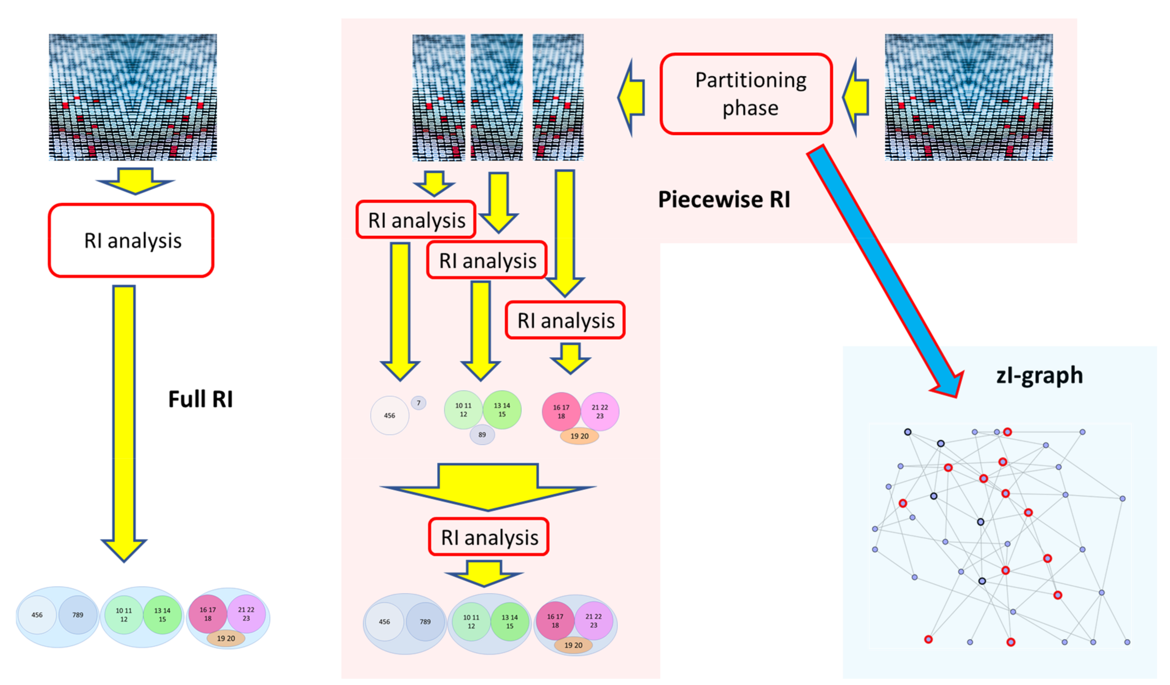
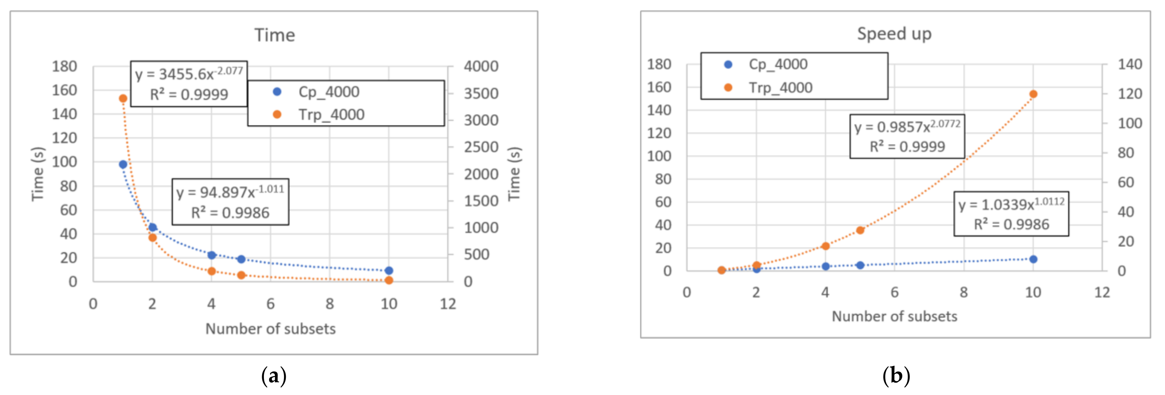
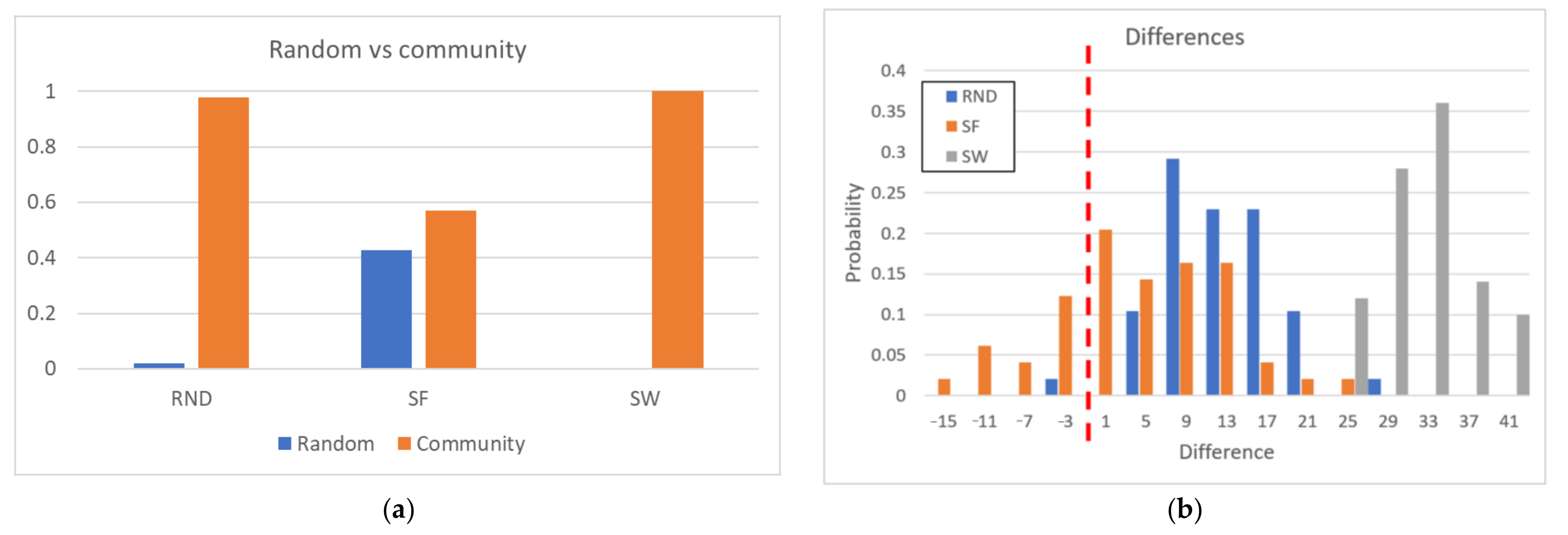
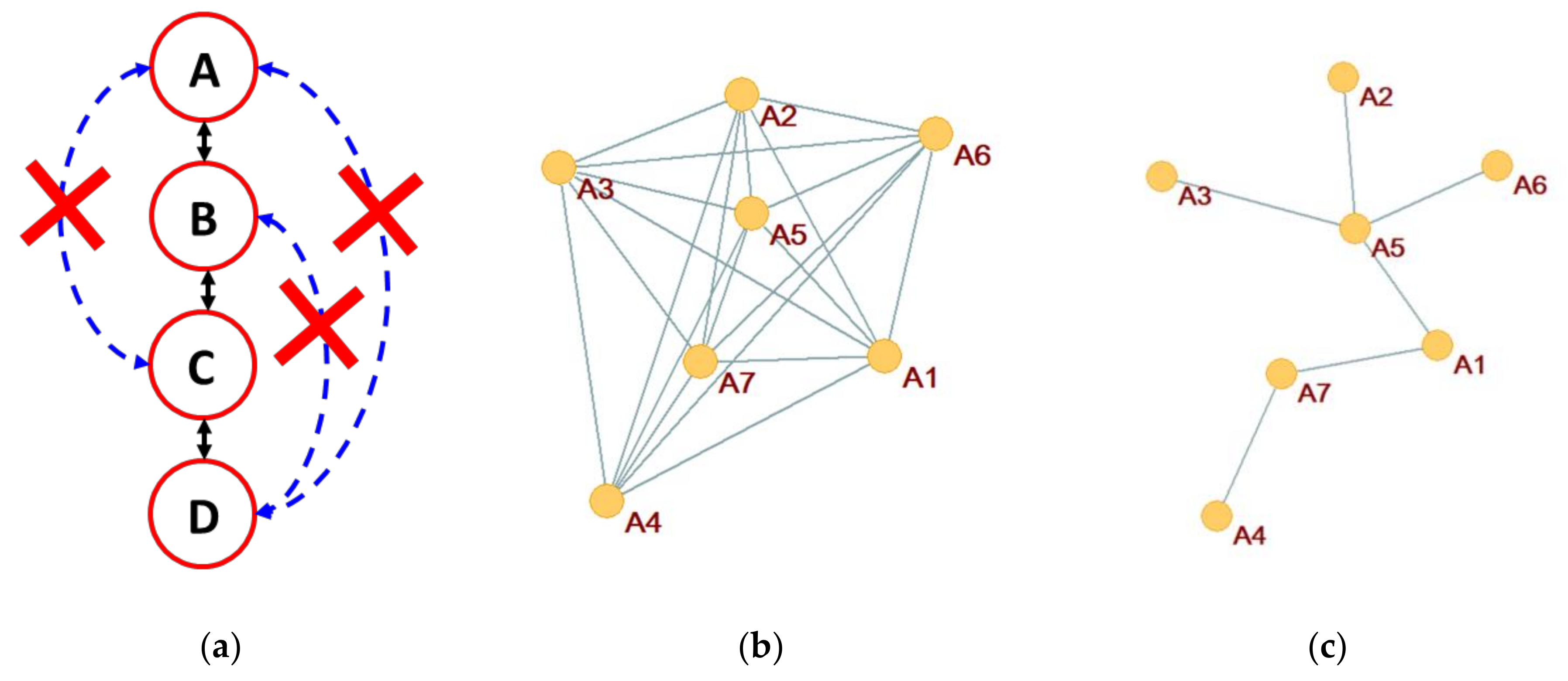
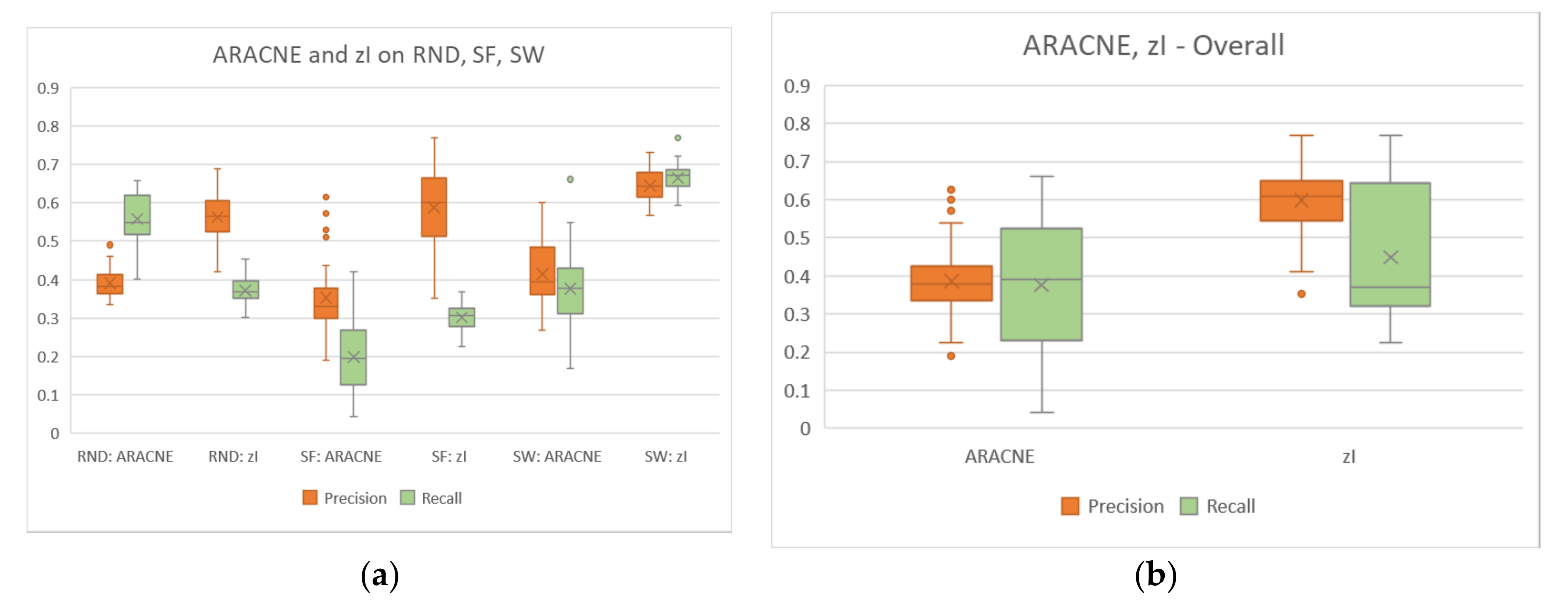
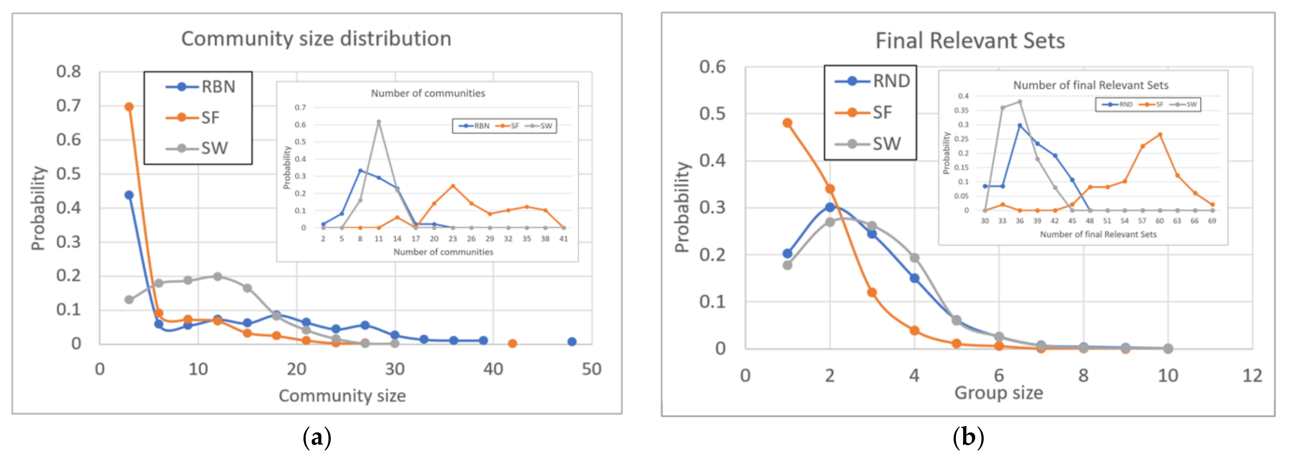
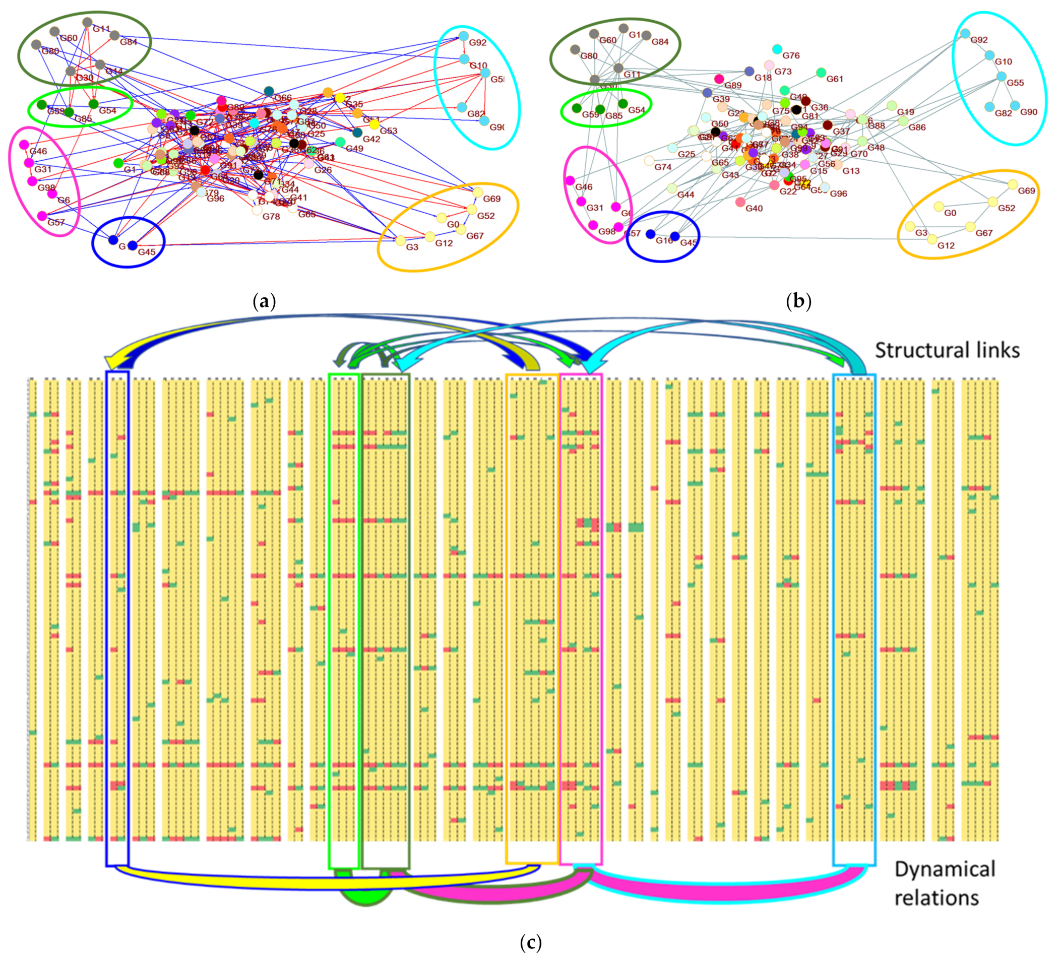
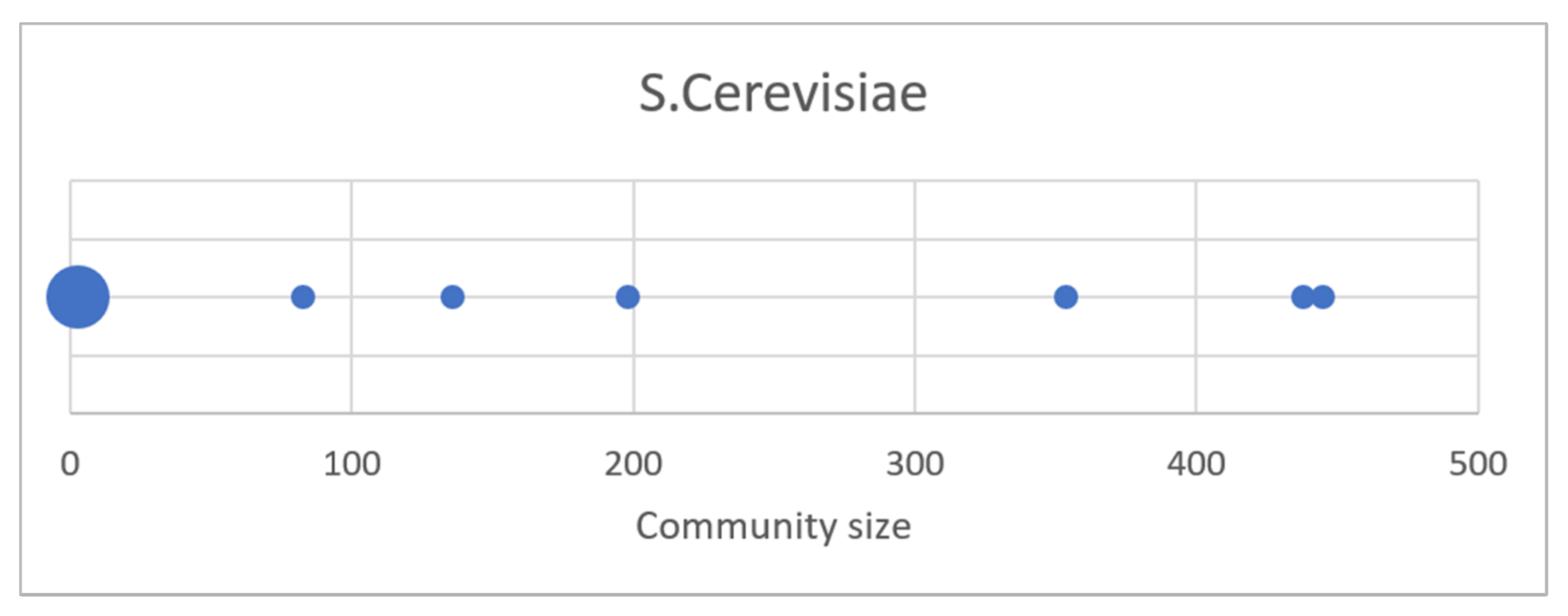
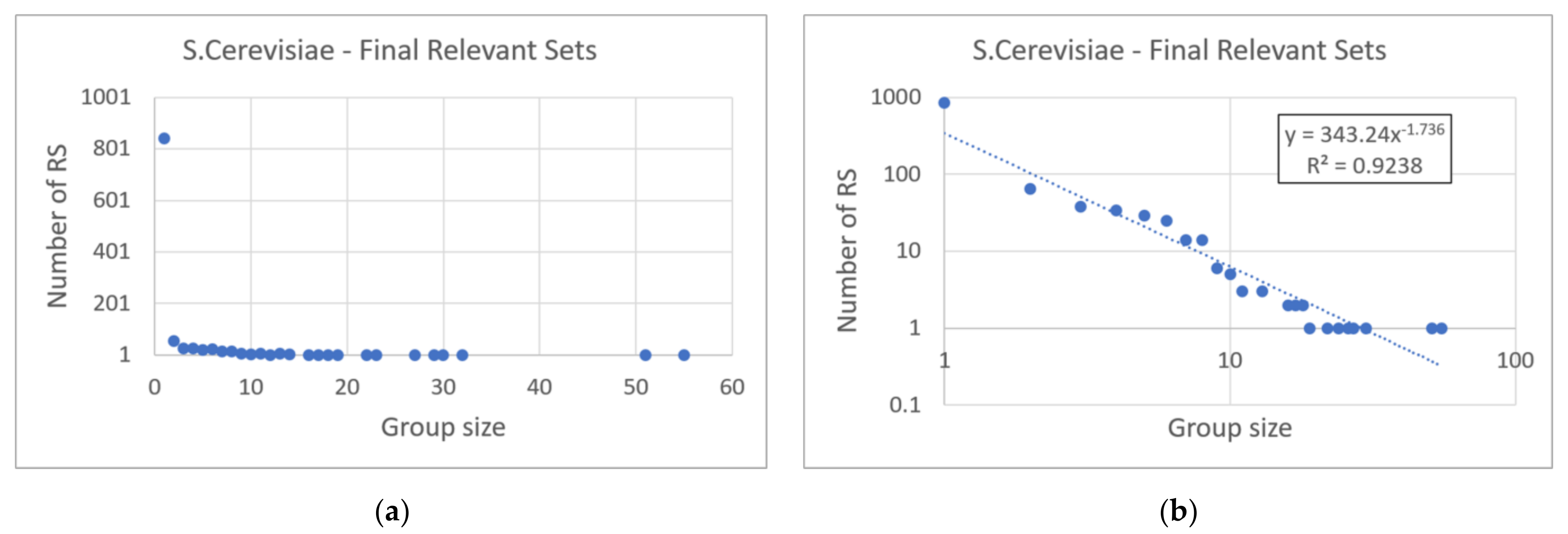
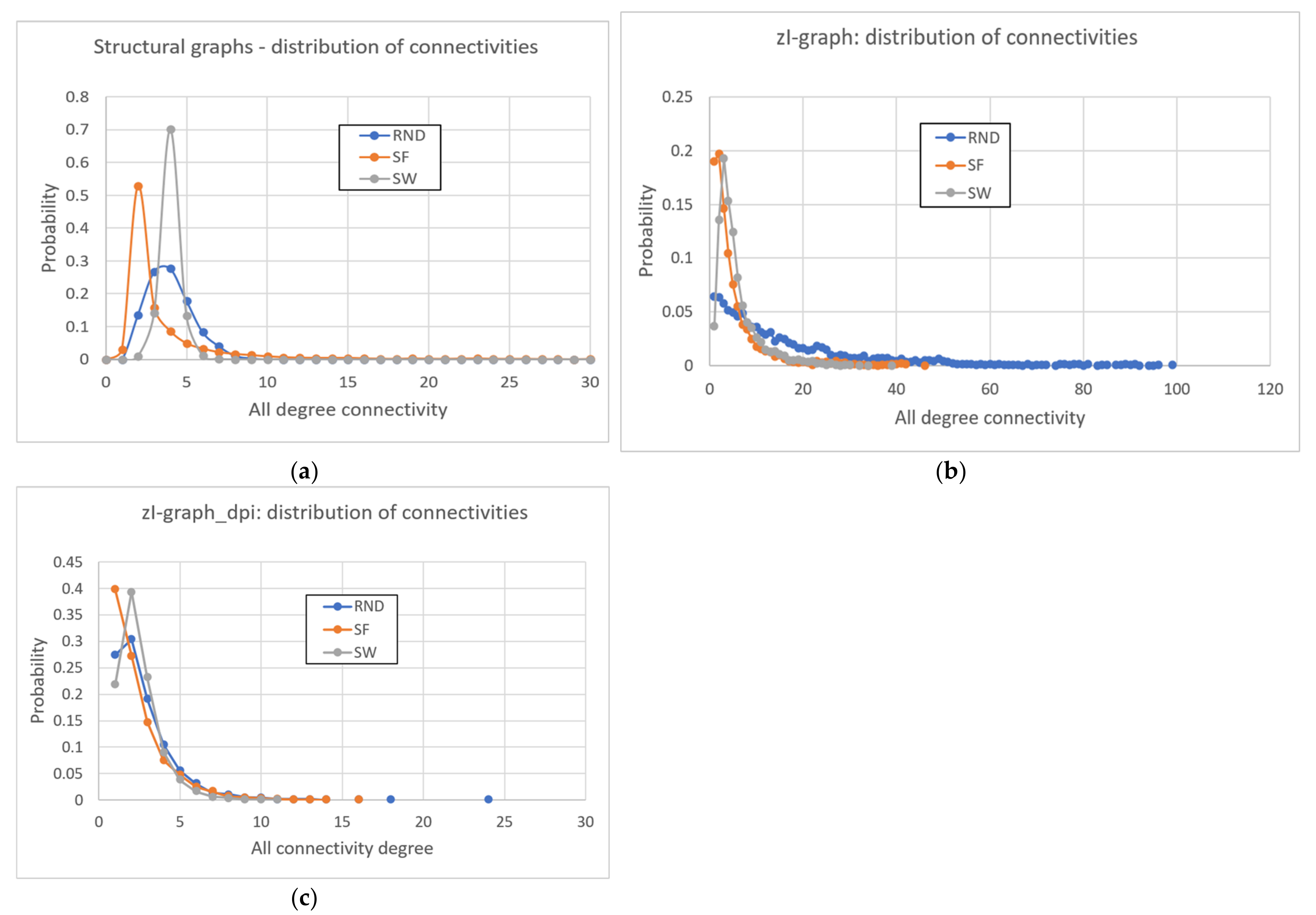
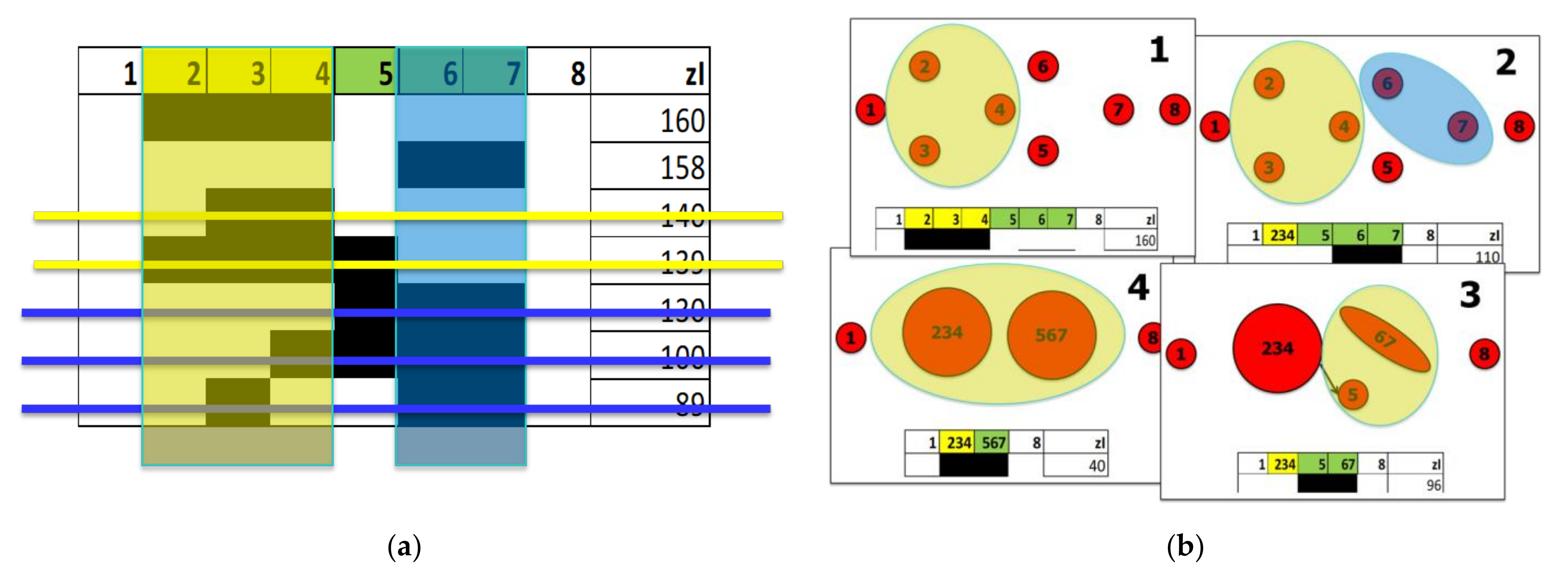
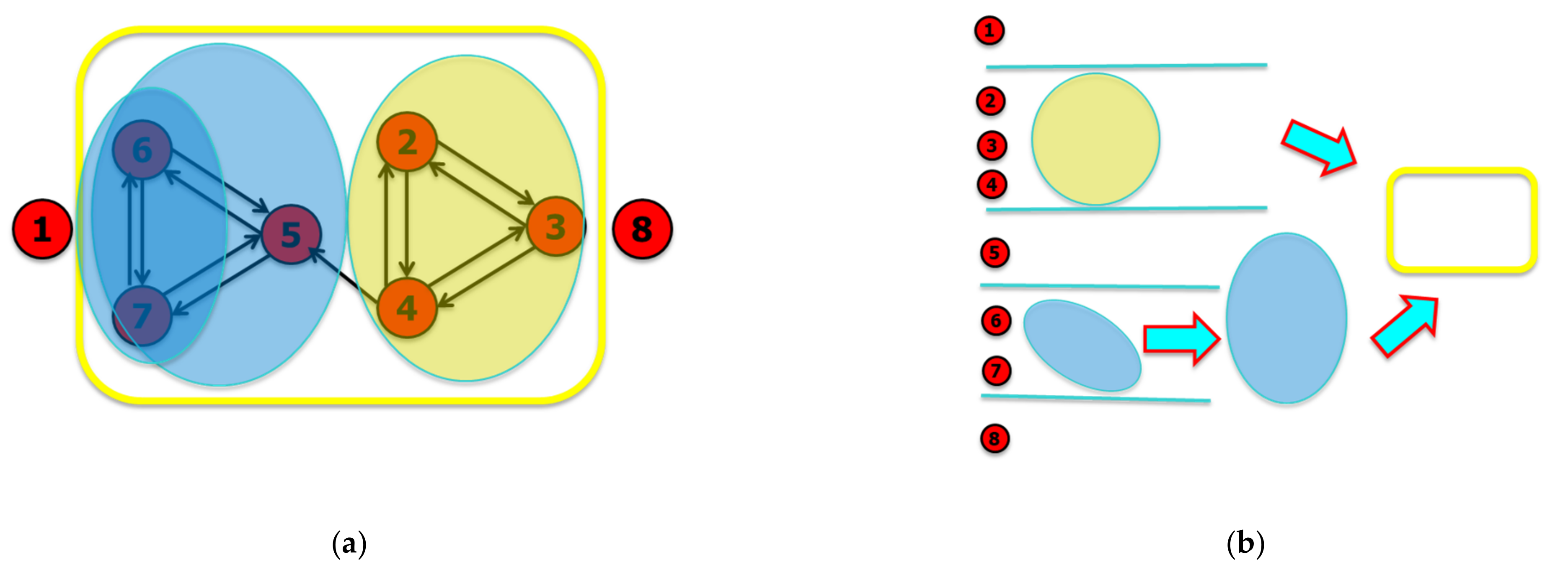
Table 1.
The results of the computation of the adjusted Rand index (ARI) among the groupings calculated by full RI method—identified here as the “ground truth”—and the corresponding groupings of the piecewise-graph RI strategy (“graph”) and of piecewise-homo RI strategy (“homo”), for the cases T_helper, CSTR, Green Community and Leader-Follower. The lines show the fraction of times the given strategy has reported an ARI exactly equal to 1.0 or greater than 0.8 and the average of the ARI index.
| Piecewise zI Strategies vs. Full zI Algorithm | Thelper | CSTR | GreenC | LF ** |
|---|---|---|---|---|
| Graph ARI = 1.0 (fraction) | 1.00 * | 1.00 * | 0.00 * | 0.95 |
| Graph ARI ≥ 0.8 (fraction) | 1.00 * | 1.00 * | 0.00 * | 1.00 |
| Graph ARI | 1.00 | 1.00 | 0.686 | 0.99 ± 0.01 |
| Homo ARI = 1.0 (fraction) | 0.70 | 0.00 | 0.00 | 0.82 ± 0.02 |
| Homo ARI ≥ 0.8 (fraction) | 0.70 | 0.00 | 0.00 | 0.95 ± 0.01 |
| Homo Average ARI | 0.82 ± 0.07 | 0.12 ± 0.06 | 0.35 ± 0.01 | 0.93 ± 0.02 |
* In the case of piecewise-graph RI strategy only one ran was made, so the fraction measurement can only have the value of 0.0 or 1.0. ** The Leader-Follower system is stochastic. We then performed 20 different runs of 150 steps each, obtaining 20 different trajectories. The table shows the average measures.
Table 2.
The results of the computation of the adjusted Rand index (ARI) among the groupings calculated by full RI method—identified here as the “ground truth”—and the corresponding groupings of the piecewise RI method, for the RND, SF and SW systems. The table shows the fraction of times the piecewise RI method reported an ARI greater than 0.8 and the average of the ARI index. The data confirms the substantial agreement of the two algorithms in the case of KOs, in some cases an almost excellent agreement (SF and SW systems).
| Piecewise zI vs. Full zI Algorithm | RND | SF | SW |
|---|---|---|---|
| ARI ≥ 0.8 (fraction) | 0.714 | 1.00 | 1.00 |
| Average ARI | 0.83 ± 0.02 | 0.960 ± 0.005 | 0.939 ± 0.006 |
Publisher’s Note: MDPI stays neutral with regard to jurisdictional claims in published maps and institutional affiliations. |
© 2021 by the authors. Licensee MDPI, Basel, Switzerland. This article is an open access article distributed under the terms and conditions of the Creative Commons Attribution (CC BY) license (https://creativecommons.org/licenses/by/4.0/).
Share and Cite
MDPI and ACS Style
D’Addese, G.; Casari, M.; Serra, R.; Villani, M. A Fast and Effective Method to Identify Relevant Sets of Variables in Complex Systems. Mathematics 2021, 9, 1022. https://0-doi-org.brum.beds.ac.uk/10.3390/math9091022
AMA Style
D’Addese G, Casari M, Serra R, Villani M. A Fast and Effective Method to Identify Relevant Sets of Variables in Complex Systems. Mathematics. 2021; 9(9):1022. https://0-doi-org.brum.beds.ac.uk/10.3390/math9091022
Chicago/Turabian StyleD’Addese, Gianluca, Martina Casari, Roberto Serra, and Marco Villani. 2021. "A Fast and Effective Method to Identify Relevant Sets of Variables in Complex Systems" Mathematics 9, no. 9: 1022. https://0-doi-org.brum.beds.ac.uk/10.3390/math9091022
Note that from the first issue of 2016, this journal uses article numbers instead of page numbers. See further details here.