Skewness-Kurtosis Model-Based Projection Pursuit with Application to Summarizing Gene Expression Data

Abstract

Non-normality is a usual fact when dealing with gene expression data. Thus, flexible models are needed in order to account for the underlying asymmetry and heavy tails of multivariate gene expression measures. This paper addresses the issue by exploring the projection pursuit problem under a flexible framework where the underlying model is assumed to follow a multivariate skew-t distribution. Under this assumption, projection pursuit with skewness and kurtosis indices is addressed as a natural approach for data reduction. The work examines its properties giving some theoretical insights and delving into the computational side in regards to the application to real gene expression data. The results of the theory are illustrated by means of a simulation study; the outputs of the simulation are used in combination with the theoretical insights to shed light on the usefulness of skewness-kurtosis projection pursuit for summarizing multivariate gene expression data. The application to gene expression measures of patients diagnosed with triple-negative breast cancer gives promising findings that may contribute to explain the heterogeneity of this type of tumors.

1. Introduction

The development of high-throughput technologies has provided the scenario to simultaneously monitor the expression levels of hundreds of genes in an attempt to obtain insights about the molecular mechanisms of human diseases. Genomic studies usually involve a vast number of measures quantifying the expression levels of genomic information from patients. An issue arising in this scenario is concerned with the data reduction through the construction of new genomic features that can summarize the expression levels of a set of genes sharing either a specific clinical characteristic or a well-established biological function. Standard methods for addressing the issue are based on first and second order moments indices using averages of expression levels and the first principal component conveying the largest variability respectively, the latter being an approach that accounts for gene dependencies provided that gene expression measures fit to the multivariate normal model. Since gene expression measures usually exhibit asymmetries and heavy tails, the normality assumption is not realistic [1,2,3,4] and dimension reduction methods based on first and second order moments entail obvious theoretical limitations. Thus, a dimension reduction approach based on higher moments is a better suited approach to capture the non-normality of this type of data. This is the motivation for exploring the skewness-kurtosis-based projection pursuit (PP) problem as a dimension reduction technique to summarize gene expression data.

This paper revisits the PP problem which in short is concerned with the search of “relevant” projections in multivariate data through the maximization of a non-normality index [5]. When the third (fourth) order moment is considered then skewness (kurtosis) is taken as projection index and the problem reduces to finding the direction that yields the maximal skewness (kurtosis) projection, an idea early proposed by [6] which has revived increasingly attention in an attempt to understand and interpret the derived projections under flexible parametric models for skewness [7,8,9,10,11,12,13,14] and kurtosis [9,15,16,17,18] indices.

The multivariate skew-t (ST) distribution has become a widely used parametric model in multivariate data analysis, due to its tractability and appealing properties, which allows the handling of asymmetry and tail weight behavior simultaneously. In this paper we propose to study the model-based PP problem under the flexible class of multivariate ST distribution using the skewness-kurtosis projection indices in the context of summarizing multivariate gene expression measures. The rest of the paper is organized as follows: Section 2 gives a general theoretical overview about the ST family and presents some motivation for its use by assessing the multivariate normality of gene expression measures from breast cancer data. Section 3 discusses the skewness-kurtosis-based PP problem under the multivariate ST model; we examine the role of the shape vector, which accounts for the non-normality the model, in the derivation of the PP direction achieving the maximal skewness-kurtosis. The theoretical results are illustrated by means of a simulation experiment with synthetic data in Section 4; the simulation experiments reveal important findings with useful implications for the application to a real gene expression cancer data set; the application is discussed in Section 5. Finally, Section 6 summarizes the main findings.

2. Background and Motivation

2.1. The Skew-Normal and Skew-T Distributions

The multivariate skew-normal (SN) distribution has become an increasingly used model that regulates departures from normality by means of a shape vector dealing with the multivariate asymmetry; its study has originated fruitful research [19,20,21,22,23,24]. In this paper we adopt the formulation given by [19,24,25] to define the density function of a normalized SN vector $\mathit{Z}$ by

$$f(\mathit{z};\mathbf{0},\mathbf{\Omega },\mathit{\alpha })=2{\varphi }_p(\mathit{z};\overline{\mathbf{\Omega }})\Phi \left({\mathit{\alpha }}^{\top }\mathit{z}\right):\mathit{z}\in {\mathbb{R}}^p,$$

(1)

where $\overline{\mathbf{\Omega }}$ is a $p\times p$ correlation matrix, ${\varphi }_p(\mathit{z};\overline{\mathbf{\Omega }})$ is the density function of a p-dimensional normal vector with zero mean and covariance matrix $\overline{\mathbf{\Omega }}$, $\Phi$ is the distribution function of a standard $N(0,1)$ variable and $\mathit{\alpha }$ is a shape $p\times 1$ vector.

To introduce location and scale parameters into this model, it is considered a location vector $\mathit{\xi }={({\xi }_1,\dots ,{\xi }_p)}^{\top }$ and a diagonal matrix $\mathit{\omega }=diag({\omega }_1,\dots ,{\omega }_p)$ with non-negative entries which converts the correlation matrix into a scale matrix $\mathbf{\Omega }=\mathit{\omega }\overline{\mathbf{\Omega }}\mathit{\omega }$; as a result, the vector $\mathit{X}=\mathit{\xi }+\mathit{\omega }\mathit{Z}$ has a SN distribution with density function

$$f(\mathit{x};\mathit{\xi },\mathbf{\Omega },\mathit{\alpha })=2{\varphi }_p(\mathit{x}-\mathit{\xi };\mathbf{\Omega })\Phi \left({\mathit{\alpha }}^{\top }{\mathit{\omega }}^{-1}(\mathit{x}-\mathit{\xi })\right):\mathit{x}\in {\mathbb{R}}^p.$$

(2)

The parameters in the density above are the location $\xi$, the scale matrix $\mathbf{\Omega }$ and the shape vector $\mathit{\alpha }$, or $\mathit{\eta }={\mathit{\omega }}^{-1}\mathit{\alpha }$, which regulates the multivariate asymmetry of the model. We write $\mathit{X}\sim S{N}_p(\xi ,\mathbf{\Omega },\mathit{\alpha })$ to denote that $\mathit{X}$ follows a SN distribution with density (2); note that when $\mathit{\alpha }=\mathbf{0}$ the multivariate normal density function is recovered.

As we know, the SN vector admits the stochastic representation: $\mathit{X}=\mathit{\xi }+\mathit{\omega }\mathit{Z}$, with $\mathit{Z}$ following a normalized skew-normal distribution with density (1). The multivariate ST distribution arises as a generalization of the SN when tail weight is injected into the model by incorporating a mixing variable S, independent of the vector $\mathit{Z}$, in the stochastic representation of the SN vector as follows: $\mathit{X}=\mathit{\xi }+\mathit{\omega }S\mathit{Z}$. The mixing variable is given by $S=V^{-1/2}$ with $V\sim {\chi }_{\nu }^2/\nu$ [26]; as a result, it can be shown that the density function of $\mathit{X}$ is

$$f(\mathit{x};\mathit{\xi },\mathbf{\Omega },\mathit{\alpha },\nu )=2t_p(\mathit{x};\nu )T_1\left({\mathit{\alpha }}^{\top }{\mathit{\omega }}^{-1}(\mathit{x}-\mathit{\xi }){\left(\frac{\nu +p}{Q_{\mathit{x}}+\nu }\right)}^{1/2};\nu +p\right):\mathit{x}\in {\mathbb{R}}^p$$

(3)

with the quantity $Q_{\mathit{x}}$ above given by $Q_{\mathit{x}}={(\mathit{x}-\mathit{\xi })}^{\prime }{\mathbf{\Omega }}^{-1}(\mathit{x}-\xi )$.

We will write $\mathit{X}\sim S{T}_p(\mathit{\xi },\mathbf{\Omega },\mathit{\alpha },\nu )$, or equivalently $\mathit{X}\sim S{T}_p(\mathit{\xi },\mathbf{\Omega },\mathit{\eta },\nu )$, to indicate that $\mathit{X}$ follows a p-dimensional ST distribution with density function (3). Please note that when $\nu \to \infty$ the ST reduces to the SN distribution, i.e., $\mathit{X}\sim S{N}_p(\mathit{\xi },\mathbf{\Omega },\mathit{\alpha })$. In addition, when $\mathit{\alpha }=\mathbf{0}$, the ST model becomes the p-dimensional t distribution for which the tail weight parameter $\nu$ controls the non-normality of the model.

2.2. Motivating Example

Cancer patients who are diagnosed with triple-negative breast cancer (TNBC) define a heterogeneous subtype of breast cancer with a worse prognosis than patients diagnosed by other cancer subtypes such as the estrogen-receptor positive ($E{R}^{+}$) or the HER2-positive. A data set containing gene expression measures for 494 TNBC patients was collected from GSE31519. An initial analysis allowed to reduce the original list with 13,146 genes to a new list containing only 1998 genes with the highest variability in their expression measures. This data set is used to illustrate the non-normality of multivariate gene expression measures.

To assess the normality assumption, we carry out multivariate normality tests for groups with $p=2,5,10$ genes. For each dimension, a subset with p genes is selected at random and the multivariate normality is assessed by the p-value of the test; the experiment is repeated 10,000 times for each one of the following tests: Shapiro-Wilk’s test [27,28], skewness and kurtosis tests implemented in the ICS R package [29], and Mardia’s [30], Henze-Zirkler’s [31], Doornik-Hansen’s tests [32] implemented in the MVN R package [33].

The results appear in

Table 1. Number of rejections of the multivariate normality assumption.

Test	$\mathit{p}=2$			$\mathit{p}=5$			$\mathit{p}=10$
	$\mathbf{\alpha }=\mathbf{0.005}$	$\mathbf{\alpha }=\mathbf{0.01}$	$\mathbf{\alpha }=\mathbf{0.05}$	$\mathbf{\alpha }=\mathbf{0.005}$	$\mathbf{\alpha }=\mathbf{0.01}$	$\mathbf{\alpha }=\mathbf{0.05}$	$\mathbf{\alpha }=\mathbf{0.005}$	$\mathbf{\alpha }=\mathbf{0.01}$	$\mathbf{\alpha }=\mathbf{0.05}$
Shapiro–Wilk’s	7716	8079	8878	9798	9853	9952	9998	9998	10,000
ICS skewness	5503	5944	7090	8583	8830	9363	9867	9904	9969
ICS kurtosis	8327	8546	9082	9934	9946	9982	10,000	10,000	10,000
Mardia skewness	5899	6368	7528	9418	9562	9812	9998	9999	10,000
Mardia kurtosis	8358	8615	9221	9958	9975	9995	10,000	10,000	10,000
Henze–Zirkler	4571	5232	6942	9200	9389	9717	9999	10,000	10,000
Doornik–Hansen	8189	8513	9135	9866	9907	9964	10,000	10,000	10,000

which displays the number of rejections for each test at significance levels: $\alpha =0.005,0.01,0.05$. We can see that the rejection is higher for the larger dimensions; overall, we can observe a great deal of rejections, even for the smallest significance level, so that it can be concluded that the multivariate normal model does not fit the gene expression measures of TNBC patients. The non-normality issue has been tackled by previous works which pointed out the cautions and caveats regarding the use of statistical methods that rely on the normality assumption [1,3].

To illustrate the suitability of non-normal multivariate distributions such as the SN and ST for modeling gene expression measures, we take the following five illustrative genes: ($GNG10,EEF1G,UQCR10,DLST,ZMYM3$). The analysis comprises the computation of the p-value for the normality tests given in Table 1 and the fit of Normal, SN and ST distributions to their expression measures by maximum likelihood using the selm function of the sn R package [34]: the p-values are $0.00803$ (Shapiro-Wilk’s), $0.00104$ (ICS skewness), 0 (ICS kurtosis), $0.02695$ (Mardia skewness), 0 (Mardia kurtosis), $0.01596$ (Henze-Zirkler) and $0.00088$ (Doornik-Hansen); the PP-plots obtained from the fit are depicted in Figure 1. The p-values are mostly against normality and the PP-plots show the adequacy of SN and ST distributions to handle the underlying non-normality of gene expression measures.

The results of our analysis reveal the limitations of the normal distribution for modeling multivariate gene expression data. Thus, we advocate for the use of more flexible models such as the SN and ST.

3. Skewness-Kurtosis Based Projection Pursuit

In this section, we study the skewness and kurtosis model-based projection pursuit problems with a goal on exploring the directions that yield the maximal skewness and kurtosis projections for a ST input vector $\mathit{X}$. From now on, it is assumed that the underlying model for the multivariate gene expression measures is a ST distribution such that $\mathit{X}\sim S{T}_p(\mathit{\xi },\mathbf{\Omega },\mathit{\eta },\nu )$ with a density function given by Equation (3). Let us denote by $\mathit{U}={\mathbf{\Sigma }}^{-1/2}(\mathit{X}-\mathit{\xi })$ its scaled version, with $\mathbf{\Sigma }$ denoting the covariance matrix of the input vector $\mathit{X}$. We study the problems for the maximization of skewness and kurtosis separately.

3.1. Skewness Maximization

Now, we consider the scaled version $\mathit{U}$ of the ST input vector. First, we address the problem of finding the direction $\mathit{c}$ for which the scalar variable $Y={\mathit{c}}^{\top }\mathit{U}$ attains the maximum skewness, as defined by the standardized third moment measure: ${\displaystyle {\gamma }_1\left(Y\right)=E^2{\left(\frac{Y-{\mu }_Y}{{\sigma }_Y}\right)}^3}$.

Since ${\gamma }_1$ is scale invariant, the search of the direction yielding the maximal skewness projection can be formulated by the following problem:

$$\underset{\mathit{c}\in {\mathbb{S}}_p}{max}{\gamma }_1\left({\mathit{c}}^{\top }\mathit{U}\right)$$

(4)

where ${\mathbb{S}}_p=\{\mathit{c}\in {\mathbb{R}}^p:{\mathit{c}}^{\top }\mathit{c}=1\}$, or equivalently by

$$\underset{\mathit{d}\in {\mathbb{S}}_p^{*}}{max}{\gamma }_1\left({\mathit{d}}^{\top }\mathit{x}\right)$$

(5)

where $\mathit{d}={\mathbf{\Sigma }}^{-1/2}\mathit{c}$ and ${\mathbb{S}}_p^{*}=\{\mathit{d}\in {\mathbb{R}}^p:{\mathit{d}}^{\top }\mathbf{\Sigma }\mathit{d}=1\}$.

The vectors providing the maximal skewness in the previous equivalent problems are denoted by

$${\mathit{\lambda }}_{skew,\mathit{X}}=\arg \underset{\mathit{d}\in {\mathbb{S}}_p^{*}}{max}{\gamma }_1\left({\mathit{d}}^{\top }\mathit{X}\right),{\mathit{\lambda }}_{skew,\mathit{U}}=\arg \underset{\mathit{c}\in {\mathbb{S}}_p}{max}{\gamma }_1\left({\mathit{c}}^{\top }\mathit{U}\right)$$

(6)

which satisfy that ${\displaystyle {\mathit{\lambda }}_{skew,\mathit{X}}\propto {\mathbf{\Sigma }}^{-1/2}{\mathit{\lambda }}_{skew,\mathit{U}}}$.

The quantity ${\displaystyle {\gamma }_{1,p}^D=\underset{\mathit{c}\in {\mathbb{S}}_p}{max}{\gamma }_1\left({\mathit{c}}^{\top }\mathit{U}\right)=\underset{\mathit{d}\in {\mathbb{S}}_p^{*}}{max}{\gamma }_1\left({\mathit{d}}^{\top }\mathit{X}\right)}$ is a well-known measure for assessing multivariate asymmetry in a directional fashion [6]. Hence, the direction driven by the vector ${\displaystyle {\mathit{\lambda }}_{skew,\mathit{X}}}$ can be used as a principal skewness direction that would allow a summary of multivariate data.

3.2. Kurtosis Maximization

When the focus is on kurtosis maximization the formulation can be established in a similar way. Now, we must find the vector $\mathit{c}$ (or $\mathit{d}$) for which the scalar variable $Y={\mathit{c}}^{\top }\mathit{U}$ (or ${\mathit{d}}^{\top }\mathit{X}$) attains the maximal kurtosis, where $\mathit{U}$ is the scaled version of the input vector $\mathit{X}$. Here, the kurtosis (excess) is quantified by the standard fourth order moment measure defined by ${\displaystyle {\gamma }_2\left(Y\right)=E{\left(\frac{Y-{\mu }_Y}{{\sigma }_Y}\right)}^4-3}$.

As in the previous case, due to the scale invariance of ${\gamma }_2$, the problem admits the following two equivalent formulations:

$$\underset{\mathit{c}\in {\mathbb{S}}_p}{max}{\gamma }_2\left({\mathit{c}}^{\top }\mathit{U}\right)$$

(7)

where ${\mathbb{S}}_p=\{\mathit{c}\in {\mathbb{R}}^p:{\mathit{c}}^{\top }\mathit{c}=1\}$, or

$$\underset{\mathit{d}\in {\mathbb{S}}_p^{*}}{max}{\gamma }_2\left({\mathit{d}}^{\top }\mathit{X}\right)$$

(8)

where $\mathit{d}={\mathbf{\Sigma }}^{-1/2}\mathit{c}$ and ${\mathbb{S}}_p^{*}=\{\mathit{d}\in {\mathbb{R}}^p:{\mathit{d}}^{\top }\mathbf{\Sigma }\mathit{d}=1\}$.

If ${\mathit{\lambda }}_{kurt,\mathit{U}}$ and ${\mathit{\lambda }}_{kurt,\mathit{X}}$ denote the vectors where the maximal kurtosis in expressions (7) and (8) is attained, respectively, then they satisfy that ${\displaystyle {\mathit{\lambda }}_{kurt,\mathit{X}}\propto {\mathbf{\Sigma }}^{-1/2}{\mathit{\lambda }}_{kurt,\mathit{U}}}$ and provide the maximal kurtosis directions. In fact, the maximal kurtosis measure ${\displaystyle {\gamma }_{2,p}^D=\underset{\mathit{c}\in {\mathbb{S}}_p}{max}{\gamma }_2\left({\mathit{c}}^{\top }\mathit{U}\right)=\underset{\mathit{d}\in {\mathbb{S}}_p^{*}}{max}{\gamma }_2\left({\mathit{d}}^{\top }\mathit{X}\right)}$ was already introduced in the past to account for the directional nature of kurtosis [6].

The main theoretical result of this work is provided by Theorem 1. It essentially states that under the flexible class of multivariate ST distributions, the vectors yielding the maximal skewness and kurtosis agree and have a simple analytical form related to the shape vector of the multivariate ST model.

Theorem 1.

Let $\mathit{X}$ be a random vector such that $\mathit{X}\sim S{T}_p(\mathit{\xi },\mathbf{\Omega },\mathit{\eta },\nu )$ with degrees of freedom $\nu >4$. Then the maximal skewness-kurtosis projections in (5) and (8) are attained at the direction of the vector: ${\displaystyle {\mathit{\lambda }}_{skew,\mathit{X}}={\mathit{\lambda }}_{kurt,\mathit{X}}=\mathit{\eta }/\sqrt{{\mathit{\eta }}^{\top }\mathbf{\Sigma }\mathit{\eta }}}$, with Σ the covariance matrix of the vector $\mathit{X}$.

Proof of Theorem 1.

See the Appendix A. □

Theorem 1 provides a revealing theoretical finding to summarize multivariate non-normality through maximal skewness-kurtosis projections; it states that the maximal non-normality is attained at the direction of the shape vector $\mathit{\eta }$ of the model since such direction not only maximizes skewness but kurtosis as well. This is also the case for vectors following a SN distribution, as stated by [9], who wondered about its validity for the ST distribution (see Section 6 in [9]). As a result, the shape vector may be interpreted as a parameter that accounts for the multivariate non-normality of the ST model in a directional way. The result also points out the parametric interpretation of the skewness-kurtosis-based PP problem under the ST distribution, a fact enhancing the inferential side of the problem which in turn poses computational implications when summarizing non-normal gene expression measures. The next section discusses in detail such computational issues giving two alternative methods for calculating maximal skewness-kurtosis projections from data.

3.3. Computational Issues

The first approach to compute the maximal non-normality direction comes from a non-parametric standpoint motivated by the representation of directional skewness as the maximum of an homogeneous third-order polynomial defined as follows [14]:

$${\gamma }_{1,p}^D=\underset{\mathit{c}\in {\mathbb{S}}_p}{max}{\gamma }_1\left({\mathit{c}}^{\top }\mathit{U}\right)=\underset{\mathit{c}\in {\mathbb{S}}_p}{max}{(\mathit{c}\otimes \mathit{c})}^{\top }{\mathit{K}}_3\left(\mathit{U}\right)\mathit{c}$$

(9)

where ${\mathit{K}}_3\left(\mathit{U}\right)$ is the $p^2\times p$ third cumulant matrix of the scaled version $\mathit{U}$ of the input vector $\mathit{X}$ and the symbol ⊗ is used to denote the tensor product.

The problem above involves an iterative numerical algorithm that requires the choice of a proper initial direction in order to avoid local maxima. The use of the right dominant eigenvector of the empirical third cumulant matrix is suggested by the higher-order power method (HOPM) as a good starting direction [35], but without providing a theoretical justification. Interestingly, when the input vector $\mathit{X}$ follows a ST distribution, it has been shown that the right dominant eigenvector of the third cumulant matrix appearing in (9) is proportional to ${\mathbf{\Sigma }}^{-1/2}\mathit{\gamma }$, with ${\displaystyle \mathit{\gamma }=\frac{\mathbf{\Omega }\mathit{\eta }}{\sqrt{1+{\mathit{\eta }}^{\top }\mathbf{\Omega }\mathit{\eta }}}}$, and also gives the direction achieving the maximal skewness projection for the scaled vector $\mathit{U}$ [14]; therefore, the maximal skewness projection for $\mathit{X}$ lies on the direction of $\mathit{\eta }$ since ${\mathbf{\Sigma }}^{-1}\mathit{\gamma }$ is proportional to $\mathit{\eta }$ —see Lemma 1 in [12]. This fact provides theoretical support for the HOPM algorithm and enhances its parametric interpretation.

The previous argument also provides the theoretical support for a non-parametric method, based on the empirical third cumulant matrix, which serves to estimate $\mathit{\eta }$ by resorting to the maximal skewness principle [14,36] as follows:

Method 1.

Estimate the skewness-kurtosis-based PP direction by means of ${\displaystyle {\widehat{\mathit{\eta }}}_1={\widehat{\mathbf{\Sigma }}}^{-1/2}\widehat{\mathit{U}}}$, where $\widehat{\mathbf{\Sigma }}$ is the sample estimate of Σ and $\widehat{\mathit{U}}$ is the right dominant eigenvector of the empirical third cumulant matrix.

A second alternative method to address the skewness-kurtosis PP problem relies on the ST assumption for the underlying distribution. As Theorem 1 shows, this assumption brings the problem to the parametric field. Therefore, we can resort to maximum likelihood (ML) for estimating the shape parameter $\mathit{\eta }$ using the functionalities of the sn R package [34]. Consequently, in order to compute the maximal non-normality projection we can use the ML method.

Method 2.

Estimate the skewness-kurtosis-based PP direction by means of ${\displaystyle {\widehat{\mathit{\eta }}}_2=\widehat{\mathit{\eta }}}$ with $\widehat{\mathit{\eta }}$ the ML estimation of the shape vector.

The next sections describe how both methods are applied. First, their performance is evaluated in a simulation study with artificial data drawn from scenarios which are designed by varying the characteristics of the underlying ST model and the sampling scheme. A real data application for the TNBC patients of the genomic experiment that motivated Section 2.2 is also provided to illustrate how they work to summarize multivariate gene expression measures.

4. Application to Synthetic Data

In this section, we carry out a simulation study to evaluate the accuracy of estimations ${\widehat{\mathit{\eta }}}_1$ and ${\widehat{\mathit{\eta }}}_2$. The experiments of the simulations are controlled by several sources that may affect the sampling behavior of the estimators. In addition to the sample size n and the dimension p of the input vector, some additional parameters $\rho$, $\tau$, $\mathbf{e}$ and the degrees of freedom $\nu$ of the ST are involved in the design of each simulation scenario: The first one, $\rho$, is used to define the correlation matrix $\overline{\mathbf{\Omega }}$ with a Toeplitz structure as follows: $\overline{\mathbf{\Omega }}={\left({\omega }_{i,j}\right)}_{1\le i,j\le p}$, with ${\omega }_{i,j}={\rho }^{|i-j|}:1\le i\le j\le p$, so that the couple $(\mathit{\omega },\rho )$ determines the scale matrix $\mathbf{\Omega }$ of the model, where $\mathit{\omega }$ must be set in advance using a well-established criterion explained in a while. Given a direction defined by a unit length vector $\mathit{e}$, asymmetry is injected into the multivariate model across the direction $\mathit{e}$ by an amount $\tau$ so that $\mathit{\alpha }=\tau \mathit{e}$. It is worthwhile noting that the couple $(\tau ,\nu )$ are non-normality indices closely related to the asymmetry and tail weight behavior of the multivariate model; they account for the non-normal features of the multivariate ST model and also determine the position of the first principal component derived from its covariance matrix. Finally, for the sake of simplicity location is set at the null vector $\mathit{\xi }=\mathbf{0}$.

Each scenario is designed by setting specific values for the aforementioned parameters. Two thousand records for the estimations of ${\widehat{\mathit{\eta }}}_1$ and ${\widehat{\mathit{\eta }}}_2$ are obtained by drawing samples of sizes $n=100,200$ from a ST distribution with the corresponding parameters. Finally, the mean square error (MSE) is calculated by comparing the unit length vectors obtained by both estimation methods with the theoretical unit norm shape vector. The simulation study is accomplished using several facilities of the sn and MaxSkew R packages [34,36].

The next sections provide an overview of the results for the bidimensional case and when the dimension is greater than two.

4.1. Simulation Study for the Bidimensional Case

Now we consider the bidimensional case; the simulation study is carried out for several scenarios defined by the following settings: $\rho =0.2,0.7$, ratio ${\omega }_2/{\omega }_1=1,2$ with $\mathit{\omega }=({\omega }_1,{\omega }_2)$, and values for the non-normality couple $(\tau ,\nu )$ equal to $(1,10)$, $(1,5)$, $(5,10)$, $(5,5)$. The results about the accuracy of both estimation methods are shown by the MSEs appearing in

Table 2. MSEs obtained from the bivariate skew-t distribution with shape vector lying on the direction of the first principal component of the scale matrix $\mathbf{\Omega }$.

	$\widehat{\mathit{\eta }}\mathit{\setminus }(\mathit{\tau },\mathit{\nu })$	(1, 10)	(1, 5)	(5, 10)	(5, 5)	(1, 10)	(1, 5)	(5, 10)	(5, 5)
		$\rho =0.2,{\omega }_2={\omega }_1$				$\rho =0.2,{\omega }_2=2{\omega }_1$
$n=100$	${\widehat{\mathit{\eta }}}_1$	0.532	0.525	0.064	0.105	0.769	0.761	0.121	0.213
	${\widehat{\mathit{\eta }}}_2$	0.491	0.368	0.022	0.012	0.789	0.604	0.034	0.031
$n=200$	${\widehat{\mathit{\eta }}}_1$	0.415	0.403	0.022	0.077	0.671	0.625	0.057	0.144
	${\widehat{\mathit{\eta }}}_2$	0.341	0.182	0.004	0.004	0.583	0.377	0.013	0.013
		$\rho =0.7,{\omega }_2={\omega }_1$				$\rho =0.7,{\omega }_2=2{\omega }_1$
$n=100$	${\widehat{\mathit{\eta }}}_1$	0.748	0.687	0.133	0.213	0.809	0.813	0.177	0.296
	${\widehat{\mathit{\eta }}}_2$	0.736	0.506	0.047	0.035	0.826	0.634	0.053	0.050
$n=200$	${\widehat{\mathit{\eta }}}_1$	0.547	0.551	0.064	0.154	0.690	0.667	0.096	0.217
	${\widehat{\mathit{\eta }}}_2$	0.478	0.281	0.012	0.013	0.573	0.422	0.021	0.021

,

Table 3. MSEs obtained from the bivariate skew-t distribution with shape vector lying on the direction of the second principal component of the scale matrix $\mathbf{\Omega }$.

	$\widehat{\mathit{\eta }}\mathit{\setminus }(\mathit{\tau },\mathit{\nu })$	(1, 10)	(1, 5)	(5, 10)	(5, 5)	(1, 10)	(1, 5)	(5, 10)	(5, 5)
		$\rho =0.2,{\omega }_2={\omega }_1$				$\rho =0.2,{\omega }_2=2{\omega }_1$
$n=100$	${\widehat{\mathit{\eta }}}_1$	0.484	0.466	0.057	0.083	0.312	0.269	0.023	0.047
	${\widehat{\mathit{\eta }}}_2$	0.445	0.341	0.013	0.007	0.296	0.175	0.007	0.004
$n=200$	${\widehat{\mathit{\eta }}}_1$	0.395	0.362	0.016	0.053	0.245	0.228	0.006	0.023
	${\widehat{\mathit{\eta }}}_2$	0.352	0.189	0.003	0.003	0.190	0.092	0.001	0.001
		$\rho =0.7,{\omega }_2={\omega }_1$				$\rho =0.7,{\omega }_2=2{\omega }_1$
$n=100$	${\widehat{\mathit{\eta }}}_1$	NA	NA	NA	NA	NA	NA	NA	NA
	${\widehat{\mathit{\eta }}}_2$	NA	NA	NA	NA	NA	NA	NA	NA
$n=200$	${\widehat{\mathit{\eta }}}_1$	0.320	0.298	0.015	0.039	0.271	0.246	0.007	0.026
	${\widehat{\mathit{\eta }}}_2$	0.300	0.231	0.002	0.002	0.260	0.148	0.002	0.001

and

Table 4. MSEs obtained from the bivariate skew-t distribution with shape vector lying on the direction of the unit vector $\mathit{e}=(0.894,0.447)$.

	$\widehat{\mathit{\eta }}\mathit{\setminus }(\mathit{\tau },\mathit{\nu })$	(1, 10)	(1, 5)	(5, 10)	(5, 5)	(1, 10)	(1, 5)	(5, 10)	(5, 5)
		$\rho =0.2,{\omega }_2={\omega }_1$				$\rho =0.2,{\omega }_2=2{\omega }_1$
$n=100$	${\widehat{\mathit{\eta }}}_1$	0.553	0.488	0.064	0.113	0.347	0.299	0.034	0.072
	${\widehat{\mathit{\eta }}}_2$	0.503	0.358	0.020	0.013	0.307	0.210	0.009	0.007
$n=200$	${\widehat{\mathit{\eta }}}_1$	0.427	0.394	0.021	0.065	0.270	0.254	0.014	0.043(0.026)
	${\widehat{\mathit{\eta }}}_2$	0.341	0.192	0.004	0.004	0.208	0.117	0.001	0.001(0.001)
		$\rho =0.7,{\omega }_2={\omega }_1$				$\rho =0.7,{\omega }_2=2{\omega }_1$
$n=100$	${\widehat{\mathit{\eta }}}_1$	0.707	0.652	0.117	0.194	0.427	0.433	0.067	0.132
	${\widehat{\mathit{\eta }}}_2$	0.607	0.484	0.034	0.029	0.395	0.338	0.011	0.012
$n=200$	${\widehat{\mathit{\eta }}}_1$	0.521	0.535	0.055	0.148	0.341	0.352	0.031	0.093(0.064)
	${\widehat{\mathit{\eta }}}_2$	0.409	0.282	0.011	0.011	0.272	0.194	0.004	0.004(0.002)

. On the other hand, additional detailed visualizations are provided by the “clock-plots” depicted in Figure 2 which display the following: the maximal non-normality direction in black, the unit length vector $\mathit{e}$ represented by the pendulum, the direction yielding the first principal component of $\mathbf{\Sigma }$ in gray, a cloud of points and finally the locations of the estimated directions ${\widehat{\mathit{\eta }}}_1$ (outer locations of the clock-plot) and ${\widehat{\mathit{\eta }}}_2$ (inner locations of the clock-plot), with the gray intensity representing in a visual way the density of directions.

When e is taken so that it lies on the direction of the first principal component of the scale matrix $\mathbf{\Omega }$, the performance of both estimations is summarized by the MSEs shown in Table 2. Overall, we can observe that the MSE increases with $\rho$ and the ratio ${\omega }_2/{\omega }_1$. As expected, the smaller MSEs are observed for the larger sample size with ${\widehat{\mathit{\eta }}}_2$ giving more accurate estimations in nearly all the cases. A revealing phenomenon is that whereas the closer scenario to multivariate normality $(\tau ,\nu )=(1,10)$ exhibits the higher errors, changes in the pair $(\tau ,\nu )$ towards non-normality give rise to remarkably higher error reductions for ${\widehat{\mathit{\eta }}}_2$, mainly in scenarios corresponding to $(\tau ,\nu )=(5,10)$ and $(\tau ,\nu )=(5,5)$; taking into account this finding, the most accurate estimations arise for the aforementioned non-normality couples when $\rho =0.2$ and ${\omega }_1={\omega }_2$. However, the MSE of ${\widehat{\mathit{\eta }}}_1$ deteriorates as we inject tail weight: we can see that for ${\widehat{\mathit{\eta }}}_2$ the MSE decreases when we departure from normality through changes in $(\tau ,\nu )$, although this is not the case for ${\widehat{\mathit{\eta }}}_1$ as shown by the peak of the MSE when $(\tau ,\nu )=(5,5)$. In short, both estimation methods may exhibit remarkable differences as it is highlighted by the top left plot displayed in Figure 2.

For the second simulation experiment, a unit length vector $\mathit{e}$ lying on the direction of the second principal component of $\mathbf{\Omega }$ is considered. The resulting MSEs obtained from both estimation methods appear reported in Table 3, with the cells containing the not available (NA) cases corresponding to situations where the ML method has failed. The reported MSEs show a slight decreasing pattern of the error with the ratio ${\omega }_2/{\omega }_1$ and an unclear pattern with respect to $\rho$. Anyway, the variability of the MSE is smaller than before with the most accurate estimations obtained for the cases $\rho =0.2$ and $\rho =0.7$ when ${\omega }_2=2{\omega }_1$ (details displayed by the top right plot of Figure 2). The other patterns we can observe for the MSE values agree qualitatively with those reported by Table 2.

Finally, if we consider the direction onto an arbitrary unit length vector given by $\mathit{e}=(0.894,0.447)$ we would obtain the results shown by Table 4. As previously, we can observe the decreasing behavior of the MSE with respect to the ratio ${\omega }_2/{\omega }_1$ and its increasing behavior against $\rho$. Once again, the most accurate estimations arise for the scenarios $(\tau ,\nu )=(5,10)$ and $(\tau ,\nu )=(5,5)$ but now when $\rho =0.2$ and ${\omega }_2=2{\omega }_1$ (see the bottom plot of Figure 2 for the detailed outcome of this simulation scenario). Other simulations, not reported here for the sake of space, have shown that the accuracy of the estimations improves as the ratio ${\omega }_2/{\omega }_1$ increases; just as an illustrative reference, Table 4 reports in parenthesis the MSEs for ${\omega }_2/{\omega }_1=3$ when $(\tau ,\nu )=(5,5)$ and $n=200$.

In summary, the simulations show that the ML method (${\widehat{\mathit{\eta }}}_2$) is more accurate than the method based on the third cumulant matrix (${\widehat{\mathit{\eta }}}_1$). Moreover, the most remarkable differences are observed as we depart from normality via asymmetry and tail weight deviations, as assessed by the parameters of the ST model.

4.2. Simulation Study for $p>2$

In this section, we address experiments with dimensions $p=5$ and $p=10$. The study only considers the settings that led to the smaller MSEs in the previous bivariate case. Hence, we will analyze the sample size $n=200$ and the non-normality couple $(\tau ,\nu )$ equal to $(5,10)$ and $(5,5)$; once again we will take $\rho =0.2,0.7$. In order to set the simulation framework, we take a first shape vector $\mathit{\alpha }$ lying on the direction of the first principal component of the scale matrix $\mathbf{\Omega }$ and another shape vector whose components are chosen arbitrarily; on the other hand, the entries of the diagonal matrix $\mathit{\omega }$ are chosen either equal to 25 or unequal with values selected at random between the integers from 1 to 35. Therefore, four simulation scenarios are set as follows:

• Scenario 1. The simulation experiments are determined by the following settings: $p=5$, shape vector lying on the direction of the first principal component of the scale matrix $\mathbf{\Omega }$, and matrix $\mathit{\omega }$ such that either $diag\left(\mathit{\omega }\right)=(25,25,25,25,25)$ or $diag\left(\mathit{\omega }\right)=(3,18,25,13,13)$, with the aforementioned values for $(\tau ,\nu )$ and $\rho$.
• Scenario 2. It is determined by the settings from the previous scenario but with the shape vector lying on the direction $\mathit{\alpha }=(1,1/2,1,1/2,1)$.
• Scenario 3. The simulation experiments are determined using the following settings: $p=10$, shape vector lying on the direction of the first principal component of the scale matrix $\mathbf{\Omega }$, and either equal diagonal elements of the matrix $\mathit{\omega }$ given by $diag\left(\mathit{\omega }\right)=(25,25,\dots ,25)$ or unequal diagonal elements given by $diag\left(\mathit{\omega }\right)=(17,10,12,33,3,9,5,30,3,16)$, with the aforementioned values for $(\tau ,\nu )$ and $\rho$.
• Scenario 4. It uses the same settings of scenario 3 but now the shape vector lies on the direction of $\mathit{\alpha }=(1,1/2,1,1/2,1,1/2,1,1/2,1,1/2)$.

Table 5. MSEs obtained for the four scenarios.

	$\widehat{\mathit{\eta }}\mathit{\setminus }(\mathit{\tau },\mathit{\nu })$	(5, 10)	(5, 5)	(5, 10)	(5, 5)	(5, 10)	(5, 5)	(5, 10)	(5, 5)
$p=5$		$\rho =0.2$		$\rho =0.2$		$\rho =0.7$		$\rho =0.7$
		Equal ${\omega }_i$		Unequal ${\omega }_i$		Equal ${\omega }_i$		Unequal ${\omega }_i$
Scenario 1	${\widehat{\mathit{\eta }}}_1$	0.198	0.393	0.650	0.954	0.462	0.784	0.853	1.117
	${\widehat{\mathit{\eta }}}_2$	0.024	0.018	0.233	0.200	0.102	0.069	0.332	0.270
Scenario 2	${\widehat{\mathit{\eta }}}_1$	0.195	0.394	0.186	0.176	0.423	0.724	0.210	0.350
	${\widehat{\mathit{\eta }}}_2$	0.022	0.018	0.025	0.003	0.098	0.067	0.026	0.012
$p=10$		$\rho =0.2$		$\rho =0.2$		$\rho =0.7$		$\rho =0.7$
		Equal ${\omega }_i$		Unequal ${\omega }_i$		Equal ${\omega }_i$		Unequal ${\omega }_i$
Scenario 3	${\widehat{\mathit{\eta }}}_1$	0.691	0.970	1.334	1.607	1.196	1.430	1.400	1.550
	${\widehat{\mathit{\eta }}}_2$	1.125	0.858	1.563	1.690	1.765	1.730	1.670	1.550
Scenario 4	${\widehat{\mathit{\eta }}}_1$	0.708	0.960	0.491	0.680	1.140	1.380	0.829	0.953
	${\widehat{\mathit{\eta }}}_2$	1.044	0.821	0.130	0.065	1.640	1.600	0.769	0.638

summarizes the accuracy of the estimations ${\widehat{\mathit{\eta }}}_1$ and ${\widehat{\mathit{\eta }}}_2$ for the simulation experiments settled in the previous scenarios.

The errors in scenario 1 show a similar behavior as in the bivariate case for both estimation methods but now higher MSEs are obtained. Overall, the higher errors are observed for the larger $\rho$ and when we take unequal ${\omega }_i$, with better MSE outcomes for ${\widehat{\mathit{\eta }}}_2$; additionally, for the heavier tail weight $\nu =5$ the MSEs of ${\widehat{\mathit{\eta }}}_1$ estimation increase while the MSE values of ${\widehat{\mathit{\eta }}}_2$ decrease slightly. The results from scenario 2, with an arbitrary shape vector, are similar to those obtained for the bidimensional case; once again, we can see a change in the behavior of the MSE with respect to the structure of the diagonal matrix $\mathit{\omega }$ (equal versus unequal ${\omega }_i$). On the other hand, as expected, the results deteriorate when $p=10$ as observed in scenarios 3 and 4: The most remarkable finding about the results in these scenarios is the high outcomes of the MSE when they are compared with the highest achievable value: $MSE=2$. Once again, we come to a similar performance of both estimation methods as in the previous scenarios, but now ${\widehat{\mathit{\eta }}}_2$ does not outperform ${\widehat{\mathit{\eta }}}_1$ in all the cases, perhaps due to the impact the higher dimension, $p=10$, has on the maximum likelihood estimation. However, such differences are not so obvious in scenario 4 whose MSE outcomes still highlight the aforementioned general behavioral pattern.

5. Application to Real Genomic Data

5.1. Data Collection

In this section, we return to the genomic study introduced in Section 2. The study collected the expression measures of 13,146 genes corresponding to 579 individuals diagnosed with a TNBC tumor; the data set is available at the Gene Expression Omnibus (GEO) repository and can be accessed through GSE31519. An amount of 85 patients who received neoadjuvant chemotherapy is removed from the analysis so that we end up with a data set containing 13,146 gene expression measures for 494 TNBC tumors samples which, after data cleaning and the retention of genes with the highest variability, gets reduced to a data set with 1998 genes and 494 TNBC samples as described in Section 2.

5.2. Application of Skewness-Kurtosis Projection Pursuit

Recent works that aim to summarize the biological underpinning of associations in genomic data have proved the usefulness of probabilistic graphical modeling (PGM) to construct association networks that reveal insights about the underlying functional biological structure responsible for the observed gene expression levels [37,38]. When applied to this genomic study, PGM gave an association network unraveling the existence of 26 gene nodes which correspond to well-defined functional biological groups as described by gene ontology [38]. Interestingly, these functional nodes are related to 15 metagenes previously described by Rody [39]; this fact deserves the construction of metanodes by grouping similar nodes within the graphical model.

Table 6. Table of Rody’s metagenes along with the corresponding genes also described in the metanodes of the probabilistic graphical model from [38].

Rody’s Metagenes	Gene Ids
Adipocyte	ADIPOQ ADH1B CD36 CHRDL1
Apocrine	PIP ALDH3B2 SPDEF FOXA1 MLPH TFAP2B AGR2 AR HMGCS2 DHRS2 UGT2B28 ALOX15B
B-Cell	IGKC IGHM IGL@ IGHG1 IGHD IGH@
Basal-Like	KRT23 SOX10 SFRP1 GABRP VGLL1 PLEKHB1 ELF5 KRT14 KRT17 KRT5 MIA KRT16 SERPINB5 S100A2 KRT6B TRIM29 KRT6A FOXC1
CLaudin-CD24	CLDN4 CLDN3 KRT19 KRT7 RAB25 CD24
HOXA	HOXA10 HOXA11
Histone	H2BFS HIST1H1C HIST1H2AE HIST1H2BG
IFN	IFI44L MX1 IFIT1 IFI27
IL-8	IL8 CXCL1 CXCL2
MHC-2	HLA-DRA HLA-DQA1 HLA-DQB1
Proliferation	CDCA8 FOXM1 BUB1
Stroma	FBN1 POSTN FN1
T-cell	GZMK PTPRC CD52

shows the correspondence between Rody’s metagenes and the representative genes from the metanodes described in [38]; note that Hemoglobin and VEGF Rody’s metagenes are excluded because they contain just a single gene from those described in [38] and here the focus is on multivariate gene expression measures.

It is well known that when gene expression measures fit the multivariate normal model, then first and second order moments will suffice to handle data variability; hence, the first component of a principal component analysis (PCA) could be a natural choice to summarize the multivariate expression measures for the genes belonging to each functional group of Table 6. However, when their expression measures exhibit departures from normality, as occurs in this case, higher-order moments will capture the variability more properly; hence, we argue that the maximal non-normality projection, based on skewness-kurtosis maximization, may be a better approach to summarizing multivariate gene expression measures in such a case. The maximal non-normality projections for each functional group in Table 6 are computed using the estimations ${\displaystyle {\widehat{\mathit{\eta }}}_1}$ and ${\displaystyle {\widehat{\mathit{\eta }}}_2}$; so we will be applying a kind of gene feature engineering.

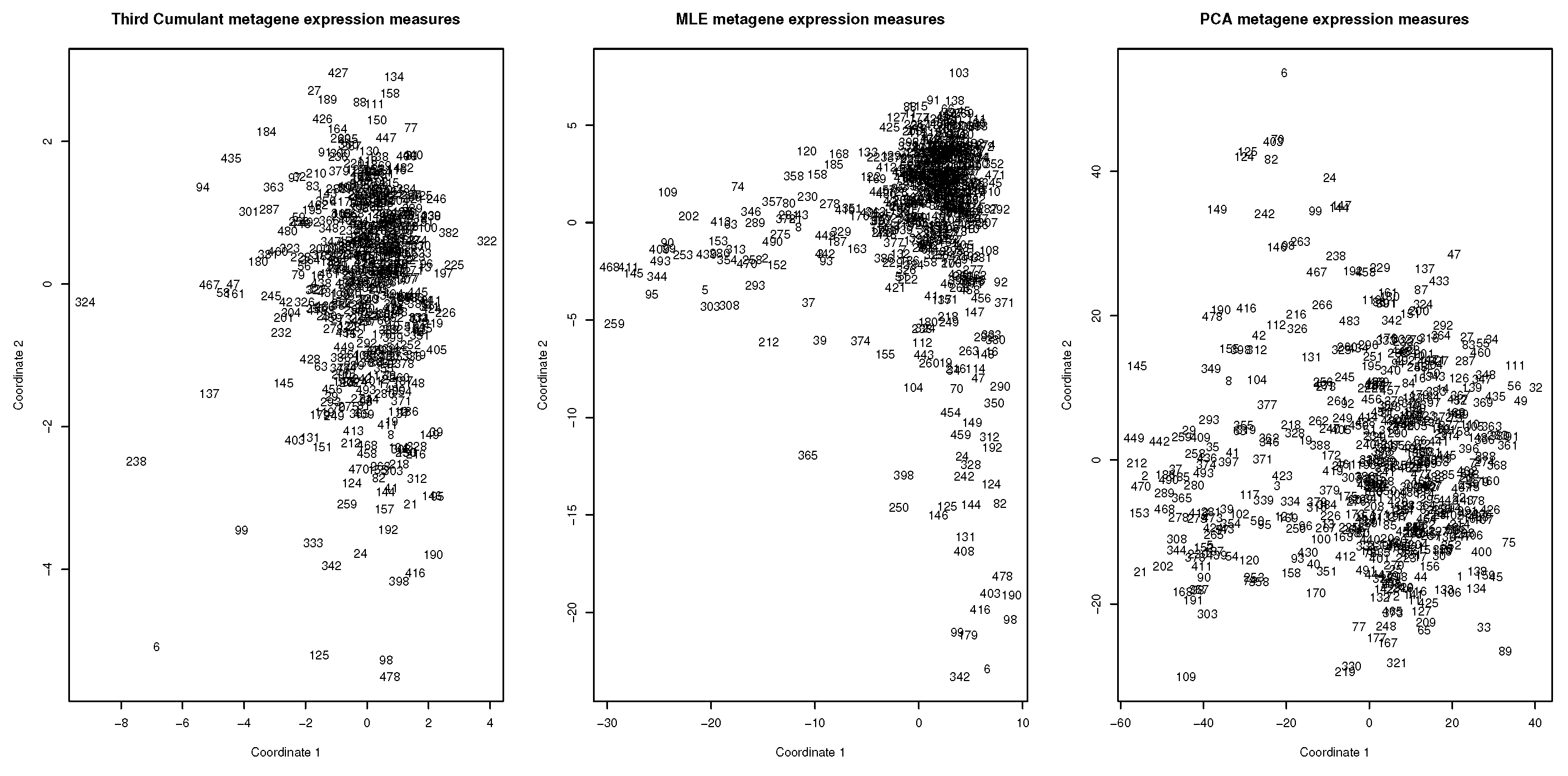
Both approaches, using PCA and skewness-kurtosis PP, provide a list with new gene features that summarize the multivariate expression measures on the basis of the prior biological functional knowledge. The derived gene features can be used as inputs for additional exploratory analysis using methods such as multidimensional scaling (MDS) which serves to represent and visualize the multivariate expression measures in a 2D coordinate system; its output gives the representation displayed by Figure 3 which clearly shows differential TNBC patterns, with an outstanding shape when the MLE method is applied.

5.3. Discussion and Interpretation of Results

To elucidate whether there may exist hidden groups in data, which may throw clues and insights about the genetic heterogeneity of TNBC patients, Gaussian mixture modeling with the BIC criterion for model selection is carried out [40,41]. The BIC criterion led to a four group model for the skewness-kurtosis PP gene features, while it resulted in three groups when PCA is used to summarize the gene expression measures. For the sake of comparison, model-based clustering with three groups for the skewness-kurtosis gene features is finally considered, with a small acceptable loss in the BIC, as provided by the model selection capabilities of the mclust R package [41]. The underlying classes have been colored by the blue, red and green colors on the display of the previous MDS visualization plots (see Figure 4). It is worthwhile noting that the skewness-kurtosis MLE projection seems to highlight a better defined class structure in data as shown in the middle plot of Figure 4.

Additional biological interpretation about the subgroups derived from the new MLE skewness-kurtosis PP gene features can be obtained using an exploratory classification tree approach to ascertain whether the resulting groups can be fully profiled through rules determined by different expression levels from the new skewness-kurtosis metagenes. The conditional inference tree method is a standard and widely used approach to achieve this goal [42,43]; an easy to use algorithm implementing the approach is provided by the partykit R package [44]. When applied to the MLE data projections, using the resulting groups as the class label for the output variable of the tree model, we obtain the tree structure displayed by Figure 5 which in turn provides a set of rules that characterize the underlying groups; it also contributes to their interpretation in terms of thresholds that highlight different over-expression conditions, shedding a flash of light in the study of the heterogeneity of TNBC patients.

It is worth noting the following revealing findings: there are two well-defined homogeneous subtypes; the first one corresponds the red group at terminal nodes 8 and 9 of the tree, the other one is the blue group which mostly appears at its terminal node 4. Thus, the first TNBC subtype would be characterized by an Apocrine over-expression as defined by the $8.407$ cutoff of the MLE Apocrine metagene; whereas, the second subtype would be characterized by an absence of over-expression in the Apocrine, Claudin and T.Cell skewness-kurtosis MLE metagenes, which is determined by expression levels under the cutoffs $8.407$, $3.074$ and $2.465$ respectively. Regarding the third TNBC subtype (green color), it can be observed that it appears mostly at the terminal nodes 5 and 6 of the tree; this finding is consistent with its heterogeneity as previously highlighted by the middle MDS plot of Figure 4. Please note that this TNBC subtype can be profiled by the absence of Apocrine over-expression and either a Claudin over-expression, associated with expression levels greater than the $3.074$ cutoff, or a T.Cell over-expression, associated with expression levels greater than the $2.465$ cutoff.

6. Concluding Remarks

This work has explored the projection pursuit problem within the framework of analyzing and summarizing gene expression data. The multivariate ST distribution arises as a flexible model for tackling the non-normality of this type of data since it can handle multivariate skewness and tail weight behavior simultaneously. In addition, projection pursuit has theoretical appealing implications when standard third and fourth moment skewness and kurtosis measures are employed as projection indices provided that the underlying model follows a multivariate ST distribution. Our theoretical findings have shown that the maximal skewness-kurtosis projection lies on the direction of the shape vector the ST distribution. As a result, two estimation methods, based on the empirical cumulant matrix (Method 1) and on the maximum likelihood approach (Method 2), have been proposed for computing such non-normality projection; their performance is evaluated through a simulation study whose outcomes show the superiority of the ML method, especially in a low-dimensional framework.

When applied to gene expression data from TNBC patients, the resulting projection pursuit directions define new gene features which contribute to reveal outstanding biological insights about the genomic heterogeneity of this type of breast cancer. More precisely, the maximal skewness-kurtosis projections help to unravel meaningful TNBC subtypes when the MLE estimation method is applied in combination with prior biological knowledge. The new skewness-kurtosis MLE gene features helped to identify three TNBC subtypes which are expected to guide pathologists, oncologists and biochemists to decipher the heterogeneity of TNBC tumors and to progress in the clinical practice accordingly.

A limitation of the skewness-kurtosis model-based projection pursuit approach is concerned with its poor performance as the dimension increases; this limitation would merit to investigate how sparse projection pursuit [45] or the graphical lasso approach to estimate the precision matrix [46,47,48] can be adapted and applied within this framework. Finally, from a theoretical standpoint, the extension of the results derived in this work to other flexible parametric families such as scale mixtures of skew-normal distributions [49] or generalized skew-normal distributions [8] may deserve further investigation; another problem for future research would lie in investigating whether it could be established a connection between previous work on multivariate skewness and kurtosis convex transform orderings [50,51,52] and the skewness-kurtosis PP problem.

References

- Hardin, J.; Wilson, J. A note on oligonucleotide expression values not being normally distributed. Biostatistics 2009, 10, 446–450. [Google Scholar] [CrossRef] [PubMed] [Green Version]
- Casellas, J.; Varona, L. Modeling Skewness in Human Transcriptomes. PLoS ONE 2012, 7, e38919. [Google Scholar] [CrossRef] [PubMed] [Green Version]
- Marko, N.F.; Weil, R.J. Non-gaussian distributions affect identification of expression patterns, functional annotation, and prospective classification in human cancer genomes. PLoS ONE 2012, 7, e46935. [Google Scholar] [CrossRef] [Green Version]
- Mar, J.C. The rise of the distributions: Why non-normality is important for understanding the transcriptome and beyond. Biophys. Rev. 2019, 11, 89–94. [Google Scholar] [CrossRef] [Green Version]
- Huber, P.J. Projection Pursuit. Ann. Stat. 1985, 13, 435–475. [Google Scholar] [CrossRef]
- Malkovich, J.F.; Afifi, A.A. On Tests for Multivariate Normality. J. Am. Stat. Assoc. 1973, 68, 176–179. [Google Scholar] [CrossRef]
- Kim, H.M.; Mallick, B.K. Moments of random vectors with skew t distribution and their quadratic forms. Stat. Probab. Lett. 2003, 63, 417–423. [Google Scholar] [CrossRef]
- Loperfido, N. Generalized Skew-Normal Distributions. In Skew-Elliptical Distributions and Their Applications: A Journey Beyond Normality; CRC/Chapman & Hall: Boca Raton, FL, USA, 2004; Chapter 4; pp. 65–80. [Google Scholar]
- Loperfido, N. Canonical transformations of skew-normal variates. Test 2010, 19, 146–165. [Google Scholar] [CrossRef]
- Loperfido, N. Skewness and the linear discriminant function. Stat. Probab. Lett. 2013, 83, 93–99. [Google Scholar] [CrossRef]
- Arevalillo, J.M.; Navarro, H. A note on the direction maximizing skewness in multivariate skew-t vectors. Stat. Probab. Lett. 2015, 96, 328–332. [Google Scholar] [CrossRef]
- Arevalillo, J.M.; Navarro, H. Data projections by skewness maximization under scale mixtures of skew-normal vectors. Adv. Data Anal. Classif. 2020, 14, 435–461. [Google Scholar] [CrossRef]
- Kim, H.M.; Kim, C. Moments of scale mixtures of skew-normal distributions and their quadratic forms. Commun. Stat. Theory Methods 2017, 46, 1117–1126. [Google Scholar] [CrossRef]
- Loperfido, N. Skewness-Based Projection Pursuit: A Computational Approach. Comput. Stat. Data Anal. 2018, 120, 42–57. [Google Scholar] [CrossRef]
- Peña, D.; Prieto, F. Cluster Identification Using Projections. J. Am. Stat. Assoc. 2001, 96, 1433–1445. [Google Scholar] [CrossRef] [Green Version]
- Peña, D.; Prieto, F. Combining Random and Specific Directions for Outlier Detection and Robust Estimation in High-Dimensional Multivariate Data. J. Comput. Graph. Stat. 2007, 16, 228–254. [Google Scholar] [CrossRef] [Green Version]
- Loperfido, N. A note on the fourth cumulant of a finite mixture distribution. J. Multivar. Anal. 2014, 123, 386–394. [Google Scholar] [CrossRef]
- Loperfido, N. Kurtosis-based projection pursuit for outlier detection in financial time series. Eur. J. Financ. 2020, 26, 142–164. [Google Scholar] [CrossRef]
- Azzalini, A.; Capitanio, A. Statistical applications of the multivariate skew normal distribution. J. R. Stat. Soc. Ser. B 1999, 61, 579–602. [Google Scholar] [CrossRef]
- Azzalini, A. The Skew-normal Distribution and Related Multivariate Families. Scand. J. Stat. 2005, 32, 159–188. [Google Scholar] [CrossRef]
- Contreras-Reyes, J.E.; Arellano-Valle, R.B. Kullback-Leibler Divergence Measure for Multivariate Skew-Normal Distributions. Entropy 2012, 14, 1606–1626. [Google Scholar] [CrossRef] [Green Version]
- Balakrishnan, N.; Scarpa, B. Multivariate measures of skewness for the skew-normal distribution. J. Multivar. Anal. 2012, 104, 73–87. [Google Scholar] [CrossRef]
- Balakrishnan, N.; Capitanio, A.; Scarpa, B. A test for multivariate skew-normality based on its canonical form. J. Multivar. Anal. 2014, 128, 19–32. [Google Scholar] [CrossRef]
- Azzalini, A.; Capitanio, A. The Skew-Normal and Related Families; IMS Monographs; Cambridge University Press: Cambridge, UK, 2014. [Google Scholar]
- Azzalini, A.; Dalla Valle, A. The multivariate skew-normal distribution. Biometrika 1996, 83, 715–726. [Google Scholar] [CrossRef]
- Azzalini, A.; Capitanio, A. Distributions generated by perturbation of symmetry with emphasis on a multivariate skew t-distribution. J. R. Stat. Soc. Ser. B 2003, 65, 367–389. [Google Scholar] [CrossRef]
- Villasenor Alva, J.A.; Estrada, E.G. A generalization of Shapiro-Wilk’s test for multivariate normality. Commun. Stat. Theory Methods 2009, 38, 1870–1883. [Google Scholar] [CrossRef]
- Gonzalez-Estrada, E.; Villasenor-Alva, J.A. goft: Tests of Fit for Some Probability Distributions; R Package Version 1.3.4. 2017. Available online: https://cran.microsoft.com/snapshot/2017-11-08/web/packages/goft/goft.pdf (accessed on 24 April 2021).
- Nordhausen, K.; Oja, H.; Tyler, D.E. Tools for Exploring Multivariate Data: The Package ICS. J. Stat. Softw. 2008, 28, 1–31. [Google Scholar] [CrossRef]
- Mardia, K.V. Applications of Some Measures of Multivariate Skewness and Kurtosis in Testing Normality and Robustness Studies. Sankhyā Indian J. Stat. Ser. B (1960–2002) 1974, 36, 115–128. [Google Scholar]
- Henze, N.; Zirkler, B. A class of invariant consistent tests for multivariate normality. Commun. Stat. Theory Methods 1990, 19, 3595–3617. [Google Scholar] [CrossRef]
- Doornik, J.; Hansen, H. An Omnibus Test for Univariate and Multivariate Normality. Oxf. Bull. Econ. Stat. 2008, 70, 927–939. [Google Scholar] [CrossRef]
- Korkmaz, S.; Goksuluk, D.; Zararsiz, G. MVN: An R Package for Assessing Multivariate Normality. R J. 2014, 6, 151–162. [Google Scholar] [CrossRef] [Green Version]
- Azzalini, A. The R Package sn: The Skew-Normal and Related Distributions such as the Skew-t (Version 1.5-2); Università di Padova: Padova, Italy, 2018. [Google Scholar]
- De Lathauwer, L.; De Moor, B.; Vandewalle, J. On the best rank-1 and rank-(R1, R2, …, RN) approximation of higher-order tensor. SIAM J. Matrix Anal. Appl. 2000, 21, 1324–1342. [Google Scholar] [CrossRef]
- Franceschini, C.; Loperfido, N. MaxSkew: Orthogonal Data Projections with Maximal Skewness; R Package Version 1.0. 2016. Available online: https://mran.microsoft.com/snapshot/2017-01-21/web/packages/MaxSkew/MaxSkew.pdf (accessed on 24 April 2021).
- Gamez-Pozo, A.; Berges-Soria, J.; Arevalillo, J.M.; Nanni, P.; Lopez-Vacas, R.; Navarro, H.; Grossmann, J.; Castaneda, C.A.; Main, P.; Diaz-Almiron, M.; et al. Combined Label-Free Quantitative Proteomics and microRNA Expression Analysis of Breast Cancer Unravel Molecular Differences with Clinical Implications. Cancer Res. 2015, 75, 2243–2253. [Google Scholar] [CrossRef] [PubMed] [Green Version]
- Prado-Vázquez, G.; Gámez-Pozo, A.; Trilla-Fuertes, L.; Arevalillo, J.M.; Zapater-Moros, A.; Ferrer-Gómez, M.; Díaz-Almirón, M.; López-Vacas, R.; Navarro, H.; Maín, P.; et al. A novel approach to triple-negative breast cancer molecular classification reveals a luminal immune-positive subgroup with good prognoses. Sci. Rep. 2019, 9, 1538. [Google Scholar] [CrossRef]
- Rody, A.; Karn, T.; Liedtke, C.; Pusztai, L.; Ruckhaeberle, E.; Hanker, L.; Gaetje, R.; Solbach, C.; Ahr, A.; Metzler, D.; et al. A clinically relevant gene signature in triple negative and basal-like breast cancer. Breast Cancer Res. 2011, 13, R97. [Google Scholar] [CrossRef] [PubMed] [Green Version]
- Fraley, C.; Raftery, A.E. Model-Based Clustering, Discriminant Analysis, and Density Estimation. J. Am. Stat. Assoc. 2002, 97, 611–631. [Google Scholar] [CrossRef]
- Scrucca, L.; Fop, M.; Murphy, T.B.; Raftery, A.E. mclust 5: Clustering, classification and density estimation using Gaussian finite mixture models. R J. 2016, 8, 205–233. [Google Scholar] [CrossRef] [Green Version]
- Hothorn, T.; Hornik, K.; Zeileis, A. Unbiased Recursive Partitioning: A Conditional Inference Framework. J. Comput. Graph. Stat. 2006, 15, 651–674. [Google Scholar] [CrossRef] [Green Version]
- Hothorn, T.; Hornik, K.; van de Wiel, M.A.; Zeileis, A. A Lego System for Conditional Inference. Am. Stat. 2006, 60, 257–263. [Google Scholar] [CrossRef] [Green Version]
- Hothorn, T.; Zeileis, A. Partykit: A Modular Toolkit for Recursive Partytioning in R. J. Mach. Learn. Res. 2015, 16, 3905–3909. [Google Scholar]
- Bickel, P.J.; Kur, G.; Nadler, B. Projection pursuit in high dimensions. Proc. Natl. Acad. Sci. USA 2018, 115, 9151–9156. [Google Scholar] [CrossRef] [Green Version]
- Meinshausen, N.; Bühlmann, P. High-dimensional graphs and variable selection with the Lasso. Ann. Stat. 2006, 34, 1436–1462. [Google Scholar] [CrossRef] [Green Version]
- Friedman, J.; Hastie, T.; Tibshirani, R. Sparse inverse covariance estimation with the graphical lasso. Biostatistics 2008, 9, 432–441. [Google Scholar] [CrossRef] [Green Version]
- Witten, D.M.; Friedman, J.H.; Simon, N. New Insights and Faster Computations for the Graphical Lasso. J. Comput. Graph. Stat. 2011, 20, 892–900. [Google Scholar] [CrossRef]
- Branco, M.D.; Dey, D.K. A General Class of Multivariate Skew-Elliptical Distributions. J. Multivar. Anal. 2001, 79, 99–113. [Google Scholar] [CrossRef] [Green Version]
- Wang, J. A family of kurtosis orderings for multivariate distributions. J. Multivar. Anal. 2009, 100, 509–517. [Google Scholar] [CrossRef] [Green Version]
- Arevalillo, J.M.; Navarro, H. A study of the effect of kurtosis on discriminant analysis under elliptical populations. J. Multivar. Anal. 2012, 107, 53–63. [Google Scholar] [CrossRef] [Green Version]
- Arevalillo, J.M.; Navarro, H. A stochastic ordering based on the canonical transformation of skew-normal vectors. Test 2019, 28, 475–498. [Google Scholar] [CrossRef]
Figure 1.
PP-plots for Normal (left), SN (middle) and ST (right) fits.
Figure 2.
Clockplots displaying the locations of the estimated directions in three scenarios: when lies on the direction of the first principal component of (top left), on the direction of the second principal component (top right) and when (bottom).
Figure 3.
MDS plots derived from the maximal non-normality gene projections, using the estimations (left) and (middle), and from the first PCA projection (right).
Figure 4.
Groups obtained from model-based clustering when applied on the maximal non-normality projections estimated by (left) and (middle), and on the first PCA projection (right).
Figure 5.
Gene expression profiles for the groups obtained by model-based clustering using the skewness-kurtosis MLE projections.