Assess the Impacts of Discount Policies on the Reliability of a Stochastic Air Transport Network

Abstract

In this study, an algorithm for reliability evaluation is proposed in order to assess the discount policy based on its effect on an air transport network. An air transport network is a typical stochastic air transport network (SATN) because its capacity (available seats) is regarded as stochastic. Under different discount policies, the term “reliability” refers to the ability to meet a certain travel demand within a limited budget. To better describe the flow of SATN, the methods of the sum of disjoint products and minimal paths are combined in the proposed algorithm. A reliability analysis is conducted at ranges of budgets and travel demands for a more accurate assessment. The outcomes of this study help the travel agents assess and select an appropriate discount policy, which is one of the important contributions. This study also contributes to enhancing the reliability fluctuation under the impact of multiple discount policies.

1. Introduction

Recently, an air transport network is more and more popular and becomes one of the crucial factors that reflects the capacity of travel agents (tour operators) to compete in the tourism industry [1,2]. The travel agents rely heavily on air transport networks to handle the transportation tasks. An air transport network can be formed as a directed graph consisting of a set of edges denoting an airport and a set of vertices representing a flight [3,4]. A flight is operated with a limited number of seats and booked by several individuals, travel agents, and other organizations. Thus, the capacity (i.e., available seats) can be regarded as stochastic quantity [5]. Herein the term “a stochastic air transport network (SATN)” refers to an air transport network.

From the service quality viewpoints, a reliable air transport network can guarantee to transport customers to their destinations smoothly. Performance evaluation for air transport networks, thus, is essential for efficient management. One of the appropriate indexes that have been substantially used is reliability, which is the ability (probability) observed in a predetermined period to perform specific tasks and functions under stated constraints [6,7]. Reliability has been concerned in terms of connectivity, travel time, and flow (capacity) reliability. Connectivity reliability is the probability of all terminals [8] or k-out-of-n terminals [9,10] to successfully connect the source with the sink. Regarding on-time performance, Bing analyzed the travel time reliability of a China aviation firm’s air transport network structure [11]. According to the proposed empirical analysis, the author provided suggestions for reliability improvement. Li et al. proposed a comprehensive model to evaluate the connectivity, capacity, and travel-time reliabilities of air traffic networks [12]. The affecting factors with their fuzziness and randomness also were considered and ranked. Another aspect is flow (capacity) reliability that considers the ability to deliver a specific demand [9,13,14,15,16,17,18,19,20]. With this in mind, several evaluation methods have been conducted in the last decade, for example, state enumeration [21,22], minimal cuts [9,13,14,15], minimal paths [15,16,17,18,19,20], cross entropy [23,24], subset simulation [25,26], and percolation theory [27,28]. State enumeration is the simplest method that enumerates entire possible network states. Minimal cuts and paths methods compute the reliability for a certain demand in terms of upper and lower boundary points, respectively. Besides, sum of the disjoint products [16,29,30,31,32], inclusion-exclusion [9,33,34], Monte Carlo simulation [17,21,35,36], and neural network [26,37] techniques are widely combined to accordingly compute the reliability. Lin et al. [16] investigated the reliability of air transport networks regarding the ability to meet travel demand within a limited time. Especially, this study mainly focused on the effects of late arrivals on reliability [16]. The evaluation algorithm was formed by the minimal path method and the sum of products technique. For reliability estimation, Khadiri and Yeh [17] applied Monte Carlo simulation to evaluate the probability for one minimal path of the network to deliver a certain amount of flow. Subset simulation focuses on the probability of small failures in the network. Percolation theory calculates the number of failures through removal progresses. Lesko et al. employed the percolation theory to analyze the fault tolerance and reliability of air transport networks [27]. The authors focused on calculating the threshold of pre-determined reliability.

When investigating the reliability, the travel agents also need to consider a budget factor for traveling as a given constraint because it is one of the sole influencing factors in the customer’s choice [38]. In fact, most customers set the amount they are willing to spend on traveling, which requires the travel agents to calculate the ability to meet demand under that budget. In real practice, travel agents often receive different discount offers from their partner airlines. More specifically, discount policies, such as quantity [39,40], trade [41], promotional [42], geographical, and seasonal discounts [43,44] often aim to increase sales, enter new markets, retain partnership and membership, encourage loyal customers, etc [45]. Obviously, the discount policies help to reduce the amount that the travel agents must pay for each flight. It, therefore, increases their ability to meet travel demands under a certain budget. However, there is no research appraising how discount policies affect air transport networks regarding reliability. Hence, there is a need to fill this gap.

This study aims to address a new approach that bases on reliability to assess the discount policy. Different from the previous study [16], this paper employs the reliability evaluation to select the policy with higher reliability. In particular, the reliability in this study refers to the probability in a specific interval for the SATN to meet travel demand within the limited budget and is evaluated under different discount policies. To achieve the stated objectives, an algorithm is built for reliability measurement and is used as a base for assessing discount policies accordingly. Even though both minimal cuts and minimal paths methods are mostly utilized for reliability assessment of stochastic flow networks [46], the minimal paths method can describe the actual flow with a time sequence well. Hence, the proposed algorithm is based on minimal paths method and the recursive sum of disjoint product (RSDP) technique [31,32]. In this study, a minimal path is redefined as a sequence of flights from the origin to the destination with no self-loop. The obtained reliability acts as a basis for the travel agent to select an appropriate discount policy for more reliable management.

In the following section, the SATN model, including major assumptions and nomenclature, is provided. A complete process to calculate the reliability of SATN is presented in Section 3. After that, Section 4 indicates how to utilize the proposed algorithm and accordingly assess the different discount policies through a numerical example. Finally, some conclusions are shown in the last section.

2. SATN Model and Reliability Evaluation

Let H ≡ (A, W, M, C) denote a SATN that includes the set of airports A, and the set of z flights W = {w_k | k = 1, 2,…, z}, the maximal capacity vector M = {M_k | k = 1, 2,…, z}, and the set of flight’s fares C = {c_k | k = 1, 2,…, z}. Each flight w_k ∈ W, is determined by its departure and arrival airport’s ($a_k$, $a_k^{*}$) departure and arrival time ($t_k$, $t_k^{*}$). Since traveling costs in this study are calculated under discount policies, the set discount rates G = {g_i | i = 1, 2,…, n}, are provided, where g_i is the discount rate for booking of i passengers, and n is the maximal capacity of all flights. In the H, X = (x₁, x₂,..., x_z) termed the capacity vector (i.e., x_k is the current capacity of the flight w_k), cannot exceed the maximal capacity vector M. Besides, the H follows some assumptions and nomenclature listed below.

2.1. Assumptions

Assumption 1.

The SATN follows the flow-conservation law.

Assumption 2.

Each flight’s capacity is independent statistically.

Assumption 3.

All flights are on-time.

In the SATN model, very few passengers get lost during their transportation by air. Thus, the SATN is said to follow the conservation law, which states that the flow-in equals the flow-out of all airports, except the origin and the destination. All flights in the SATN are considered separate flights. It means that their capacities are independent statistically. According to the correlation between flights that are carried by the same aircraft, their capacity and corresponding capacity will be the same. Besides, this study aims to figure out the impacts of discount policies instead of late arrivals; thus, all flights are assumed to be on time.

2.2. Nomenclature

X ≤ Y	(x1, x2,..., xz) ≥ (y1, y2,..., yz) if xk ≥ yk for all k
X < Y	(x1, x2,..., xz) > (y1, y2,..., yz) if X ≥ Y and exists at least one xh > yh
X ≹ Y	neither X ≥ Y nor X < Y

Let X = (x₁, x₂,..., x_z) and Y = (y₁, y₂,..., y_z), which are two different capacity vectors of the SATN. Since being z-vectors, they are equal if and only if x_k = y_k for k = 1, 2,…, z. Therefore, X ≤ Y when x_k ≥ y_k for all z states k. If existing at least one state x_h > y_h, X becomes greater than Y. On other hand, neither X ≥ Y nor X < Y if there is at least one state that x_h < y_h and x_k ≥ y_k for the remaining states.

3. Reliability Assessment

The classical definition of reliability is the ability (probability) to successfully fulfill the requirements under specific constraints. More specifically, the SATN reliability refers to the probability that at least (E) passengers can be transported from the origin (o) to the destination (d) within the limited budget (B) in a specific interval. Let Λ contain all capacity vectors (Ys), such that SATN can transport at least E passengers to the destination d from the origin o within the limited budget B. The SATN reliability can be computed through the formula $R_{EB}={\displaystyle {\sum }_{Y\in \Lambda }\mathrm{Pr}(Y)}$. However, under a large and complex H, the number of feasible capacity vectors (Y ∈ Λ) increases dramatically; thus, it becomes hard to enumerate them and to sum up their corresponding probabilities. For more efficiency, the SATN reliability can be derived via the lower and upper boundary points [47,48]. In which any capacity vector (Y ∈ Λ) is between at least one upper boundary point and at least one lower boundary point. Note that the maximal capacity vector (M) is the only upper boundary point and the lower boundary point is defined as follows.

Definition 1.

X is one of the lower boundary points if X ∈ Λ and there is no Y ∈ Λ that Y < X.

Let Ξ_L consist of all lower boundary points. The SATN reliability formula becomes:

$$R_{EB}=\mathrm{Pr}\left\{{\displaystyle \underset{X\in E_L}{\cup }\left\{Y\right|X\le Y\le M\}}\right\}$$

(1)

According to Equation (1), figuring out the set Ξ_L is necessary for computing reliability. Inferred from Definition 1, any X = (x₁, x₂,..., x_z) ∈ Ξ_L must satisfy the following three conditions.

Condition 1.

At least E passengers can be transported from the origin o to the destination d under it,

Condition 2.

The traveling costs do not exceed the limited budget B,

Condition 3

There is no Y ∈ Λ that Y < X.

3.1. Minimal Paths and Feasible Flow Vectors

Regarding Condition 1, that guarantees the transportation from the origin o to the destination d, we first search all minimal paths that are sequences of flights where the first flight departs at the origin o and the last flight arrives at the destination d with no self-loop and named MPs herein. Note that, passengers will be transported through one MP that can accommodate any flight, as long as that its first flight departs at the origin o and its last flight arrives at the destination d with no self-loop. Thus, each MP can be a sequence of one to z flights, whose flights must ensure the order of visiting airports and departure/arrival times. Suppose that P₁, P₂,..., P_m are all MPs of the SATN. Let F = (f₁, f₂,..., f_m) be a flow vector where f_j denotes the flow on P_j for j = 1, 2,…, m.

Following the flow-conservation law, the total flow through any w_k cannot exceed its maximal capacity M_k.

$$M_k\ge {\displaystyle \sum _j\left\{f_j\right|w_k\in P_j)\}},\mathrm{for}k=1,2,\dots ,z.$$

(2)

Similarly, a flow vector F is feasible under X if and only if

$$x_k\ge {\displaystyle \sum _j\left\{f_j\right|w_k\in P_j)\}},\mathrm{for}k=1,2,\dots ,z.$$

(3)

For example, if there are three MPs P₁, P₂, and P₃ going through flight w_k, a flow vector F = (f₁, f₂,..., f_m) must satisfy that x_k ≥ f₁ + f₂ + f₃. Also, a capacity vector X is feasible under F if x_k ≥ f₁ + f₂ + f₃. Let V(X) = $\max {\displaystyle \sum _{j=1}^m\left\{f_j\right|}$F is feasible under X} be the maximum flow under X. Using V(X), condition 1 becomes.

V(X) ≥ E.

(4)

The following lemma indicates the necessary conditions for a capacity vector X meeting condition 1.

Lemma 1.

X meets Condition 1 if there exists at least one F such that

$$M_k\ge x_k\ge {\displaystyle \sum _j\left\{f_j\right|w_k\in P_j)\}},\mathrm{for}k=1,2,\dots ,z.$$

(5)

$${\displaystyle \sum _{j=1}^m{f}_j}=E.$$

(6)

Proof. 

Let F = {Fs satisfy Constraints (5) and (6)}. Constraint (5) said that such flow vectors F ∈ F are feasible under X. Therefore, V(X) = $\max {\displaystyle \sum _{j=1}^m\left\{f_j\right|}$F ∈ F} and the following constraint is inferred:

$${\displaystyle \sum _{j=1}^m{f}_j}\le V\left(X\right)$$

(7)

Combining with Constraint (6), we have:

$$E\le V\left(X\right)$$

(8)

Lemma 1 is proved.

3.2. Traveling Costs under Discount Policies

This subsection focuses on Condition 2—finding all capacity vectors whose traveling costs after discounted, named $c_j^o(X)$ where o denotes the discount policy, do not exceed the limited budget B.

$$c_j^o(X)>B,\mathrm{for}\mathrm{all}\left\{j\right|f_j>0\}.$$

(9)

Among several discount policies offered by airlines, quantity and contractual discounts are only ones the travel agent can take advantage of. Therefore, they are focused on this study.

Policy 1. Quantity discount (i.e., a discount is granted for purchasing large quantities) aims to encourage bulk bookings. The higher volume the travel agents book, the higher discount rates the airlines offer.

Policy 2. Contractual discount (i.e., partnership discount, a discount is offered to partners for the functions they perform) provides the travel agents a specific discount rate no matter how much they book on each flight. It, normally, depends on the terms signed and/or the cooperation between two sides: travel agent and airlines.

Because two different discount policies are considered, this study provides two corresponding formulas to calculate the traveling cost $c_j^o(X)$ of capacity vector X on P_j. Under policy 1, the discount rate depends on the booking quantity. Therefore, we have:

$$c_j^1(X)={\displaystyle \sum _{k|k\in P_j}\{c_k\times (1-g_i|i=x_k)\}},\mathrm{for}\left\{j\right|f_j>0\}.$$

(10)

On the other hand, policy 2 offers a fixed discount rate. For a more accurate assessment, the authors pick up one the discount rate from G and call it g. The following equation is for the calculation of the traveling costs under policy 2.

$$c_j^2(X)={\displaystyle \sum _{k|k\in P_j}\{c_k\times (1-g)\}},\mathrm{for}\left\{j\right|f_j>0\}.$$

(11)

3.3. Generate All Lower Boundary Points

Combining the former subsections, a capacity vector X ∈ Λ if it satisfies Constraint (9) and exists at least one F ∈ F feasible under it. The following property adds condition 3 to determine lower boundary point candidates.

Lemma 2.

If X ∈ Ξ_L then exists F ∈ F such that

$$x_k={\displaystyle \sum _j\left\{f_j\right|w_k\in P_j)\}},\mathrm{for}k=1,2,\dots ,z.$$

(12)

Proof. 

Suppose that Y = (y₁, y₂,..., y_z) and X = (x₁, x₂,..., x_z)∈ Ξ_L. Obviously, both X and Y ∈ Λ. Suppose to exist a capacity of X satisfying that $M_t\ge x_t>{\displaystyle \sum _j\left\{f_j\right|w_k\in P_j)\}}$ and $x_k={\displaystyle \sum _j\left\{f_j\right|w_k\in P_j)\}}$ for k ≠ t where $y_t={\displaystyle \sum _j\left\{f_j\right|w_k\in P_j)\}}$ and $y_k={\displaystyle \sum _j\left\{f_j\right|w_k\in P_j)\}}$ for k ≠ t. It indicates that Y < X, which conflicts with condition 3. Hence, $x_k={\displaystyle \sum _j\left\{f_j\right|w_k\in P_j)\}}$, for k = 1, 2,…, z. Lemma 2 is proved.

Lemma 2 indicates that all capacity vectors X converted from Fs ∈ F through Equation (12) and satisfies Constraint (9) are lower boundary point candidates. Let Ξ contain all of them. The set Ξ_L of all exact lower boundary points is obtained by rejecting from Ξ all capacity vector Y if existing any X < Y.

3.4. Solution Procedure

Given the SATN H ≡ (A, W, M, C), travel demand E, transit time θ, limited budget B with the set of quantity discount rates G, the origin o, and the destination d, the main algorithm is proposed for reliability evaluation as follows.

• Step 1: Generate all feasible minimal paths (MPs) as follows.

  Set j = 1, Ω = Ø, Ə = {o}, and, μ = length(Ə)//*j is an index of a feasible MP (Pj), Ω stores Pj’s flights, and Ə stores airports that Pj visits. Function Search (Ω, Ə, o, d, μ, θ)
  (1.1)	IF μ ≠ 1, let wh be the μ–1th element of Ω Select one available flight wk such that $a_k$ ≡ $a_h^{*}$ and $a_k^{*}$∉ Ə
  (1.2)	IF $t_k$≥ $t_k^{*}$ + θ
  (1.3)	Ω ← Ω ∪ {wk}, Ə ← Ə ∪ {$a_k^{*}$}, and μ = μ + 1
  (1.4)	IF $a_k^{*}$ = d then Pj ← Ω, output Pj, j = j + 1
  (1.5)	ELSE, Call search (Ω, Ə, o, d, μ, θ)
  (1.6)	ELSE, select one available flight wk that departs from o
  (1.7)	Go to step (1.2)
  (1.8)	Ω ← Ω\{wk}, Ə ← Ə\{$a_k^{*}$}, and μ = μ − 1
  (1.9)	Next selection
  (1.10)	END

Suppose that Step 1 accepted m MPs: P₁, P₂,..., P_m.

• Step 2: Through the following equation, obtain set F of all flow vectors F fulfilling the travel demand E.

  $${\displaystyle \sum _{j=1}^m{f}_j}=E.$$

  (13)

  $${\displaystyle \sum _j\left\{f_j\right|w_k\in P_j)\}}\le M_k,\mathrm{for}k=1,2,\dots ,z.$$

  (14)
• Step 3: Through Equation (15), convert each flow vector F ∈ F into capacity vector X and store it in Δ.

  $$x_k={\displaystyle \sum _j\left\{f_j\right|w_k\in P_j)\}},\mathrm{for}k=1,2,\dots ,z.$$

  (15)
• Step 4: Calculate the traveling cost of capacity vector X ∈ Δ on MPs.
• (4.1) Under policy 1:

  $$c_j^1(X)={\displaystyle \sum _{k|k\in P_j}\{c_k\times (1-g_i|i=x_k)\}},\mathrm{for}\left\{j\right|f_j>0\}.$$

  (16)
• (4.2) Under policy 2:

  $$c_j^2(X)={\displaystyle \sum _{k|k\in P_j}\{c_k\times (1-g)\}},\mathrm{for}\left\{j\right|f_j>0\}.$$

  (17)

Then, reject from Δ any capacity vectors that exceed does not exceed the limited budget to get two corresponding sets ${\Xi }^o$, for o = 1, 2, of all lower boundary point candidates.

$${\Xi }^o=\mathsf{\Delta }\backslash \left\{X\right\}\mathrm{if}{c}_j^o(X)>B,\mathrm{for}\left\{j\right|f_j>0\}.$$

(18)

• Step 5: Through the following comparison process, obtain a set ${\Xi }_L^o$ of all exact lower boundary points from ${\Xi }^o$ for o = 1, 2.

  Initially, Θ stores θ indexes of Xs in ${\Xi }^o$
  (5.1)	FOR k = 1 to θ ∈ Θ
  (5.2)	FOR h = k + 1 to θ ∈Θ
  (5.3)	IF Xk ≤ Xh then Xh is not a lower boundary point, Θ = Θ\{h} ELSE IF Xk > Xh then Xk is not a lower boundary point, Θ = Θ\{k}, and BREAK
  (5.6)	${\Xi }_L^o$ = {Xk| k ∈Θ}

• Step 6: Compute the reliability as Equation (19) by utilizing the RSDP algorithm [31,32].

  $$R_{EB}^o=\mathrm{Pr}\left\{{\displaystyle \underset{X\in {\Xi }_L^o}{\cup }\left\{Y\right|M\ge Y\ge X\}}\right\},\mathrm{for}o=1,2.$$

  (19)

Basically, the main algorithm is developed according to lemmas and statements in the former subsections. It first searches all minimal paths, then generates all lower boundary points and utilizes the RSDP method to calculate the reliabilities.

4. A Numerical Example and Reliability Analysis

To demonstrate how the main algorithm runs and assess the impacts of two different discount policies on the reliability, this section adopts the SATN of a travel agent Y from Vietnam to be a numerical example. To transport customers to Taipei (TPE) from Da Nang (DAD), the Y agent has contracted some airlines and airports in Hanoi (HAN) and Ho Chi Minh city (SGN) to build up their SATN, shown in

Table 1. The discount rates for all flights of the SATN.

Capacity	(i)	1	2	3	4	5
Quantity Discount Rate	(gi)	0.05	0.075	0.1	0.15	0.2

and

Table 2. The relevant information about all flights of the SATN.

Flight	Fare	Departure Time	Arrival Time	Departure—Arrival Airport	Probability Pr (xk)
wk	ck	tk	$t_k^{*}$	(ak–$a_k^{*}$)	xk = 5	xk = 4	xk = 3	xk = 2	xk = 1	xk = 0
1	900	7:00	8:00	DAD-HAN	0.81	0.1	0.05	0.02	0.01	0.01
2	900	9:45	10:45	DAD-HAN	0.80	0.1	0.05	0.02	0.01	0.02
3	950	7:15	8:30	DAD-SGN	0.81	0.05	0.06	0.05	0.01	0.02
4	950	10:15	11:30	DAD-SGN	0.80	0.08	0.05	0.05	0.01	0.01
5	1200	8:45	10:15	HAN-SGN		0.935	0.035	0.01	0.01	0.01
6	1200	9:00	10:30	SGN-HAN		0.94	0.04	0.005	0.005	0.01
7	3250	11:00	14:30	HAN-TPE	0.81	0.1	0.05	0.02	0.01	0.01
8	3250	11:30	15:00	SGN-TPE	0.90	0.055	0.02	0.01	0.005	0.01

.

4.1. Evaluate the Reliability of Numerical Example

Given travel demand E = 5 (passengers), and limited budget B = 5000 Taiwan dollar (TWD), the discount rate of contractual policy g = g₂, the reliabilities $R_{EB}^o$ for o = 1, 2 are evaluated by the following steps.

• Step 1: Generate all feasible minimal paths (MPs). Totally, four MPs: P₁ = {w₁, w₅, w₈}, P₂ = {w₁, w₇}, P₃ = {w₃, w₆, w₇}, P₄ = {w₃, w₈} are accepted.
• Step 2: Through Equations (20) and (21), obtain set F of all flow vectors F fulfilling the travel demand E

  $$f_1+f_2+f_3+f_4=5.$$

  (20)

  $$f_1+f_2\le 5;f_1+f_2\le 5;f_1\le 4;f_3\le 4;f_2+f_3\le 5;f_1+f_4\le 5.$$

  (21)

All obtained flow vectors are shown in column 1 of

Table 3. The results of four steps (2)–(5).

Step 2		Step 3		Step 4.1	Step 4.2	Step 5
(F)		(Δ)		(${\mathit{\Xi }}^1$)	$\left({\mathit{\Xi }}^2\right)$	$\left({\mathit{\Xi }}_{\mathit{L}}^1\right)$	$\left({\mathit{\Xi }}_{\mathit{L}}^2\right)$
F1 =	(0, 0, 0, 5)	X1 =	(0, 0, 5, 0, 0, 0, 0, 5)	√	√	√	√
F2 =	(0, 0, 1, 4)	X2 =	(0, 0, 5, 0, 0, 1, 1, 4)	√	√	√	√
…
F6 =	(0, 1, 0, 4)	X6 =	(1, 0, 4, 0, 0, 0, 1, 4)	√	√	√	√
F7 =	(0, 1, 1, 3)	X7 =	(1, 0, 4, 0, 0, 1, 2, 3)	√	√	√	√
…
F11 =	(0, 2, 1, 2)	X11 =	(2, 0, 3, 0, 0, 0, 2, 3)	√	√	√	√
F12 =	(1, 0, 1, 3)	X12 =	(2, 0, 3, 0, 0, 1, 3, 2)	√	√	√	√
…
F22 =	(1, 0, 1, 3)	X22 =	(1, 0, 4, 0, 1, 1, 1, 4)	$c_3^1(X_{12})$ = 5036	√	$c_3^1(X_{12})>B$	X22 > X6
F23 =	(1, 0, 2, 2)	X23 =	(1, 0, 4, 0, 1, 2, 2, 3)	√	√	X23 > X7	X23 > X7
…
F26 =	(1, 1, 0, 3)	X26 =	(2, 0, 3, 0, 1, 0, 1, 4)	√	√	√	√
F27 =	(1, 1, 1, 2)	X27 =	(2, 0, 3, 0, 1, 1, 2, 3)	$c_1^1(X_{27})$ = 5001	√	$c_1^1(X_{27})$ > B	X27 > X11
F28 =	(1, 1, 2, 1)	X28 =	(2, 0, 3, 0, 1, 2, 3, 2)	√	√	X28 > X12	X28 > X12
…
F37 =	(2, 0, 1, 2)	X37 =	(2, 0, 3, 0, 2, 1, 1, 4)	$c_1^1(X_{37})$ = 5083	√	$c_1^1(X_{37})$ > B	X37 > X26
F38 =	(2, 0, 2, 1)	X38 =	(2, 0, 3, 0, 2, 2, 2, 3)	√	√	X38 > X11	X38 > X11
F39 =	(2, 0, 3, 0)	X39 =	(2, 0, 3, 0, 2, 3, 3, 2)	√	√	X39 > X12	X39 > X12
…
F54 =	(4, 1, 0, 0)	X54 =	(5, 0, 0, 0, 4, 0, 1, 4)	√	√	√	√

.

• Step 3: Through Equation (22), convert each flow vector F ∈ F into capacity vector X and store it in Δ, referring to column 2 of Table 3.

  $$x_1=f_1+f_2;x_3=f_1+f_2;x_5=f_1\le 4;x_6=f_3;x_7=f_2+f_3;x_8=f_1+f_4.$$

  (22)
• Step 4: Calculate the traveling cost of each capacity vector X ∈ Δ on MPs. Then, reject from Δ any capacity vectors through Constraints (24) and (26) to get corresponding sets of all lower boundary point candidates under policies 1 and 2.
• (4.1) Under policy 1:

  $$c_j^1(X)={\displaystyle \sum _{k|k\in P_j}\{c_k\times (1-g_i|i=x_k)\}},\mathrm{for}\left\{j\right|f_j>0\}.$$

  (23)

  $${\Xi }^1=\mathsf{\Delta }\backslash \left\{X\right\}\mathrm{if}{c}_j^1(X)>B,\mathrm{for}\left\{j\right|f_j>0\}.$$

  (24)

  For instance, since F₂₂ > 0, it is necessary to check the traveling cost of X₂₂ = (1, 0, 4, 0, 1, 1, 1, 4) on P₁, P₃, and P₄. By means of Equation (23), we have: $c_1^1(X)=c_1\times (1-g_1)+c_5\times (1-g_1)+c_8\times (1-g_4)=$900*0.95 + 1200*0.95 + 3250*0.85 = 4758. Similarly, $c_3^1(X)=5036$ and $c_4^1(X)=3571$.
• (4.2) Under policy 2:

  $$c_j^2(X)={\displaystyle \sum _{k|k\in P_j}\{c_k\times (1-g)\}},\mathrm{for}\left\{j\right|f_j>0\}.$$

  (25)

  $${\Xi }^2=\mathsf{\Delta }\backslash \left\{X\right\}\mathrm{if}{c}_j^2(X)>B,\mathrm{for}\left\{j\right|f_j>0\}.$$

  (26)

  Columns 3 and 4 of Table 3 present sets ${\Xi }^1$ and ${\Xi }^2$, respectively, and one of the reasons for each rejection.
• Step 5: Through the following comparison process, obtain the sets of all exact lower boundary points ${\Xi }_L^1$ = ${\Xi }_L^2$ = {X₁, X₂,…, X₂₁, X₂₆, X₃₀, X₃₃, X₃₅, X₃₆, X₄₀, X₄₃, X₄₅, X₄₆, X₄₉, X₅₁, X₅₂, X₅₄}. Column 5 of Table 3 remarks why a certain X does not belong to ${\Xi }_L^1$ or/and ${\Xi }_L^2$.
• Step 6: Utilize the RSDP algorithm into Equation (27) to compute the reliabilities under two policies.

  $$R_{EB}^1=R_{EB}^2=\mathrm{Pr}\left\{{\displaystyle \underset{i=1}{\overset{54}{\cup }}\left\{Y\right|M\ge Y\ge X_i\}}\right\}$$

  (27)

In terms of the RSDP technique, the reliability in this case is the sum of 54 terms $R_{EB}^1=R_{EB}^2={\displaystyle \sum _{i=1}^{54}Term\_i}$ where Term_1 is Pr(Y|M ≥ Y ≥ X₁) for i = 1, and Term_i = Pr(Y|M ≥ Y ≥ X_i) − Pr{(Y|M ≥ Y ≥ max(X₁, X_i))∪…∪(Y|M ≥ Y ≥ max(X_i-1, X_i))} for 54 ≥ i ≥ 2.

Because ${\Xi }_L^1$ = ${\Xi }_L^2$, we have $R_{EB}^1$ = $R_{EB}^2$ = 0.98755955. This reliability means that the travel agent does not meet only one or two in a hundred offers. It indicates a high possibility to transport five passengers with no more than 5000 TWD. There is no reliability difference in the reliability between applying quantity discounts and contractual discounts where g = g₂.

4.2. Analyze the Impact of Discount Policies on the Reliability

Focusing on the impact of different discount policies, this section considers all discount rates. Besides, the authors evaluate the reliabilities of different travel demands and limited budgets.

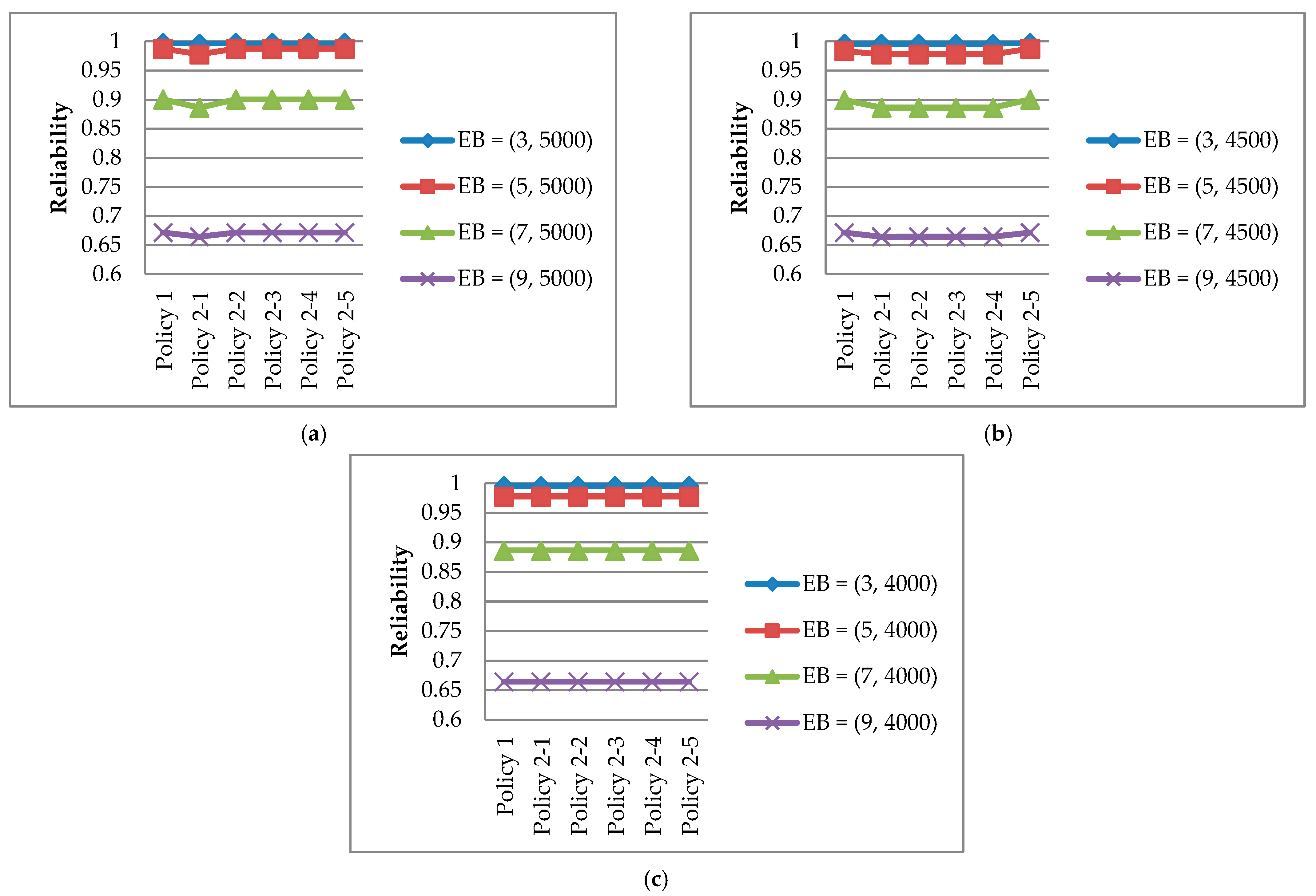
As shown in Figure 1 and

Table 4. The reliabilities of SATN subject to ranges of travel demands and limited budgets (E, B).

Travel Demand and Limited Budget EB = (E, B)	Policy 1 Quantity Discount	Policy 2 Contractual Discount
		g = g1	g = g2	g = g3	g = g4	g = g5
EB = (3, 5000)	0.99786556	0.99591643	0.99787289	0.99787289	0.99787289	0.99787289
EB = (5, 5000)	0.98755955	0.97779929	0.98755955	0.98755955	0.98755955	0.98755955
EB = (7, 5000)	0.90026408	0.8862315	0.90026408	0.90026408	0.90026408	0.90026408
EB = (9, 5000)	0.67142394	0.66424293	0.67142394	0.67142394	0.67142394	0.67142394
EB = (3, 4500)	0.99591643	0.99591643	0.99591643	0.99591643	0.99591643	0.99787289
EB = (5, 4500)	0.98335734	0.97779929	0.97779929	0.97779929	0.97779929	0.98755955
EB = (7, 4500)	0.89911623	0.8862315	0.8862315	0.8862315	0.8862315	0.90026408
EB = (9, 4500)	0.67142394	0.66424293	0.66424293	0.66424293	0.66424293	0.67142394
EB = (3, 4000)	0.99591643	0.99591643	0.99591643	0.99591643	0.99591643	0.99591643
EB = (5, 4000)	0.97779929	0.97779929	0.97779929	0.97779929	0.97779929	0.97779929
EB = (7, 4000)	0.8862315	0.8862315	0.8862315	0.8862315	0.8862315	0.8862315
EB = (9, 4000)	0.66424293	0.66424293	0.66424293	0.66424293	0.66424293	0.66424293

, regardless of whether the travel agent selects policy 1 or 2, the reliabilities with B = 4000 TWD are the same. However, the travel agent must receive a discount rate g ≥ g₂ for the same reliability under policy 1 when B = 5000 TWD. Under policy 2 with B = 4500 TWD, they even need the highest discount to keep the reliabilities at the same or slightly greater.

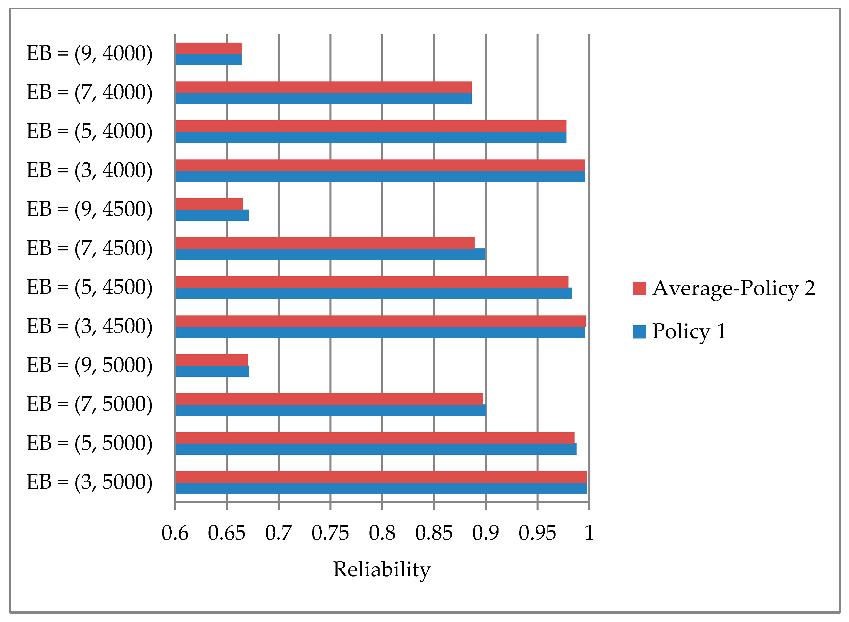
Besides, this study calculates the average of the reliabilities under policy 2 then compares them with that under policy 1 at each travel demand and limited budgets. The comparison results are presented in Figure 2. It is clear that the reliability under policy 1 is not lower than the average reliability under policy 2 at all 12 levels of demands and budgets. Policy 1 also has more positive effects in the cases that the limited budgets B = 4500 and B = 5000 TWD.

Though the differences are not great, the travel agent can conclude that the quantity discount policy is a relatively better choice as it gets greater or similar reliabilities in most cases. The travel agent can also determine the most beneficial option, exactly. For example, with a limited budget B = 5000 TWD, if the discount rate offered is 0.05 then the quantity discount policy is the right choice. However, they should choose the contractual discount policy if airlines increase their discount rate to about 0.175. Besides, the travel agent knows that alternatives or adjustments are needed for higher reliability since the reliabilities of their SATN at the travel demand E = 9 are low, despite applying discount policies.

5. Conclusions

This paper focuses on reliability evaluation for an air transport network and uses it as a base to assess the impact of different discount policies. The most positive influencing policy is recommended as an appropriate choice towards more reliable performance. To accomplish this aim, a stochastic air transport network (SATN) is formulated as a typical directed graph. Then, an algorithm, based on the minimal paths (MP) method, is proposed to simultaneously calculate the SATN reliability under the impact of quantity and contractual discounts. Whilst it has been proved that finding all feasible MPs in a complex network like the SATN belongs to an NP-hard problem [49], this study provides an evaluation algorithm without assuming that all MPs are known.

Furthermore, a numerical example is carried out applying the proposed algorithm to investigate the reliability of the SATN under different discount policies. The fluctuation of reliability is examined, subject to travel demands and budget, to make a broader assessment. Some potential management actions are also suggested. In short, this research provides a new approach that takes discount policy under consideration in reliability evaluation and examines the effects of different policies. Likewise, other transport networks can employ the proposed algorithm to address the same issues: reliability evaluation and the definition of optimal discount policies with the limited budget and given demand.

In the future, there is potential to assess the impacts of discount policies based on reliability estimation in the case of demand uncertainty or lacking probability data [50,51,52]. Also, addressing the same research problem with the dependent capacity [53] can get more realistic findings.

References

- Rocha, L.E. Dynamics of air transport networks: A review from a complex systems perspective. Chin. J. Aeronaut. 2017, 30, 469–478. [Google Scholar] [CrossRef]
- Eggenberg, N.; Salani, M.; Bierlaire, M. Constraint-specific recovery network for solving airline recovery problems. Comput. Oper. Res. 2010, 37, 1014–1026. [Google Scholar] [CrossRef]
- Du, W.-B.; Zhou, X.-L.; Lordan, O.; Wang, Z.; Zhao, C.; Zhu, Y.-B. Analysis of the Chinese Airline Network as multi-layer networks. Transp. Res. Part E Logist. Transp. Rev. 2016, 89, 108–116. [Google Scholar] [CrossRef] [Green Version]
- Zhou, Q.; Yang, W.; Zhu, J. Mapping a Multilayer Air Transport Network with the Integration of Airway, Route, and Flight Network. J. Appl. Math. 2019, 2019, 1–10. [Google Scholar] [CrossRef]
- Lin, Y.-K. Stochastic flow networks via multiple paths under time threshold and budget constraint. Comput. Math. Appl. 2011, 62, 2629–2638. [Google Scholar] [CrossRef] [Green Version]
- Choy, K.; Sheng, N.; Lam, H.; Lai, I.K.; Chow, K.; Ho, G. Assess the effects of different operations policies on warehousing reliability. Int. J. Prod. Res. 2014, 52, 662–678. [Google Scholar] [CrossRef]
- Todinov, M.T. 8—Reliability Networks. In Flow Networks: Analysis and Optimization of Repairable Flow Networks, Networks with Disturbed Flows, Static Flow Networks and Reliability Networks; Todinov, M., Ed.; Elsevier: Oxford, UK, 2013; pp. 143–166. ISBN 978-0-12-398396-1. [Google Scholar]
- Karger, D.R. A randomized fully polynomial time approximation scheme for the all terminal network reliability problem. In Proceedings of the Twenty-Seventh Annual ACM Symposium on Theory of Computing—STOC ’95, Las Vegas, NV, USA, May 29–June 1 1995; pp. 11–17. [Google Scholar] [CrossRef] [Green Version]
- Yeh, W.-C. A simple algorithm for evaluating the k-out-of-n network reliability. Reliab. Eng. Syst. Saf. 2004, 83, 93–101. [Google Scholar] [CrossRef]
- Habib, A.; Al-Seedy, R.; Radwan, T. Reliability evaluation of multi-state consecutive k-out-of-r-from-n: G system. Appl. Math. Model. 2007, 31, 2412–2423. [Google Scholar] [CrossRef]
- Bing, D. Reliability Analysis for Aviation Airline Network Based on Complex Network. J. Aerosp. Technol. Manag. 2014, 6, 193–201. [Google Scholar] [CrossRef] [Green Version]
- Li, S.; Zhang, Z.; Cheng, X. Reliability Analysis of an Air Traffic Network: From Network Structure to Transport Function. Appl. Sci. 2020, 10, 3168. [Google Scholar] [CrossRef]
- Younes, A.; Girgis, M.R. A tool for computing computer network reliability. Int. J. Comput. Math. 2005, 82, 1455–1465. [Google Scholar] [CrossRef]
- Lin, Y.-K. Performance index of a stochastic-flow network with node failure under the budget constraint. Int. J. Adv. Manuf. Technol. 2006, 31, 1209. [Google Scholar] [CrossRef]
- Datta, E.; Goyal, N.K. Reliability estimation of stochastic flow networks using pre-ordered minimal cuts. In Proceedings of the 2016 International Conference on Microelectronics, Computing and Communications (MicroCom), Durgapur, India, 23–25 January 2016; pp. 1–6. [Google Scholar]
- Lin, Y.-K.; Nguyen, T.-P.; Yeng, L.C.-L. Reliability evaluation of a multi-state air transportation network meeting multiple travel demands. Ann. Oper. Res. 2019, 277, 63–82. [Google Scholar] [CrossRef]
- El Khadiri, M.; Yeh, W.-C. An efficient alternative to the exact evaluation of the quickest path flow network reliability problem. Comput. Oper. Res. 2016, 76, 22–32. [Google Scholar] [CrossRef]
- Lin, Y.-K.; Huang, C.-F. Stochastic computer network under accuracy rate constraint from QoS viewpoint. Inf. Sci. 2013, 239, 241–252. [Google Scholar] [CrossRef]
- Khanna, G.; Chaturvedi, S.; Soh, S. On computing the reliability of opportunistic multihop networks with Mobile relays. Qual. Reliab. Eng. Int. 2019, 35, 870–888. [Google Scholar] [CrossRef]
- Christodoulou, S.E.; Fragiadakis, M.; Agathokleous, A.; Xanthos, S. Chapter 5—Vulnerability Assessment of Water Distribution Networks Under Seismic Loads. In Urban Water Distribution Networks: Assessing Systems Vulnerabilities, Failures, and Risks; Christodoulou, S.E., Fragiadakis, M., Agathokleous, A., Xanthos, S., Eds.; Butterworth-Heinemann: Oxford, UK, 2018; pp. 173–207. ISBN 978-0-12-813652-2. [Google Scholar]
- Hou, K.; Jia, H.; Yu, X.; Zhu, L.; Xu, X.; Li, X. An impact increments-based state enumeration reliability assessment approach and its application in transmission systems. In Proceedings of the 2016 IEEE Power and Energy Society General Meeting (PESGM), Boston, MA, USA, 17–21 July 2016; pp. 1–5. [Google Scholar]
- Liu, X.; Hou, K.; Jia, H.; Mu, Y.; Ma, S.; Wang, F.; Lei, Y. The Impact-increment State Enumeration Method Based Component Level Resilience Indices of Transmission System. Energy Procedia 2019, 158, 4099–4103. [Google Scholar] [CrossRef]
- Mattrand, C.; Bourinet, J.-M. The cross-entropy method for reliability assessment of cracked structures subjected to random Markovian loads. Reliab. Eng. Syst. Saf. 2014, 123, 171–182. [Google Scholar] [CrossRef]
- Caserta, M.; Nodar, M.C. A cross entropy based algorithm for reliability problems. J. Heuristics 2009, 15, 479–501. [Google Scholar] [CrossRef]
- Au, S.-K.; Beck, J.L. Estimation of small failure probabilities in high dimensions by subset simulation. Probabilistic Eng. Mech. 2001, 16, 263–277. [Google Scholar] [CrossRef] [Green Version]
- Papadopoulos, V.; Giovanis, D.G.; Lagaros, N.D.; Papadrakakis, M. Accelerated subset simulation with neural networks for reliability analysis. Comput. Methods Appl. Mech. Eng. 2012, 223–224, 70–80. [Google Scholar] [CrossRef]
- Lesko, S.; Aleshkin, A.; Zhukov, D. Reliability Analysis of the Air Transportation Network when Blocking Nodes and/or Connections Based on the Methods of Percolation Theory. IOP Conf. Series Mater. Sci. Eng. 2020, 714, 012016. [Google Scholar] [CrossRef]
- Kong, Z.; Yeh, E.M. Correlated and cascading node failures in random geometric networks: A percolation view. In Proceedings of the 2012 Fourth International Conference on Ubiquitous and Future Networks (ICUFN), Phuket, Thailand, 4–6 July 2012; pp. 520–525. [Google Scholar]
- Yeh, W.-C. An improved sum-of-disjoint-products technique for the symbolic network reliability analysis with known minimal paths. Reliab. Eng. Syst. Saf. 2007, 92, 260–268. [Google Scholar] [CrossRef]
- Yeh, W.-C. An Improved Sum-of-Disjoint-Products Technique for Symbolic Multi-State Flow Network Reliability. IEEE Trans. Reliab. 2015, 64, 1185–1193. [Google Scholar] [CrossRef]
- Bai, G.; Zuo, M.J.; Tian, Z. Ordering Heuristics for Reliability Evaluation of Multistate Networks. IEEE Trans. Reliab. 2015, 64, 1015–1023. [Google Scholar] [CrossRef]
- Zuo, M.J.; Tian, Z.; Huang, H.-Z. An efficient method for reliability evaluation of multistate networks given all minimal path vectors. IIE Trans. 2007, 39, 811–817. [Google Scholar] [CrossRef]
- Lin, Y.-K. Reliability of a stochastic-flow network with unreliable nodes and cost constraints. In Proceedings of the 11th ISSAT International Conference on Reliability and Quality in Design, St. Louis, MO, USA, 4–6 August 2005; pp. 83–86. [Google Scholar]
- Huang, D.-H.; Huang, C.-F.; Lin, Y.-K. Reliability Evaluation for a Stochastic Flow Network Based on Upper and Lower Boundary Vectors. Mathematics 2019, 7, 1115. [Google Scholar] [CrossRef] [Green Version]
- Jiang, Y.; Li, R.; Kang, R.; Huang, N. The method of network reliability and availability simulation based on Monte Carlo. In Proceedings of the 2012 International Conference on Quality, Reliability, Risk, Maintenance, and Safety Engineering, Chengdu, China, 15–18 June 2012; pp. 245–250. [Google Scholar]
- Zhao, X.; Wang, D.; Yan, Y.; Gu, Z. Stochastic Simulation on System Reliability and Component Probabilistic Importance of Road Network. Math. Probl. Eng. 2015, 2015, 1–5. [Google Scholar] [CrossRef]
- Cheng, C.-S.; Hsu, Y.-T.; Wu, C.-C. Fault modeling and reliability evaluations using artificial neural networks. In Proceedings of the Proceedings of ICNN’95—International Conference on Neural Networks, Perth, WA, Australia, 27 November–1 December 2002; Volume 1, pp. 427–432. [Google Scholar]
- O’Connell, J.F.; Williams, G. Passengers’ perceptions of low cost airlines and full service carriers: A case study involving Ryanair, Aer Lingus, Air Asia and Malaysia Airlines. J. Air Transp. Manag. 2005, 11, 259–272. [Google Scholar] [CrossRef] [Green Version]
- Qiu, X.; Lee, C.-Y. Quantity discount pricing for rail transport in a dry port system. Transp. Res. Part E Logist. Transp. Rev. 2019, 122, 563–580. [Google Scholar] [CrossRef]
- Liu, H.; Lobschat, L.; Verhoef, P.C.; Zhao, H. The effect of permanent product discounts and order coupons on purchase incidence, purchase quantity, and spending. J. Retail. 2020. [Google Scholar] [CrossRef]
- Xu, X.; Chen, R.; Zhang, J. Effectiveness of trade-ins and price discounts: A moderating role of substitutability. J. Econ. Psychol. 2019, 70, 80–89. [Google Scholar] [CrossRef]
- Gauri, D.K.; Ratchford, B.; Pancras, J.; Talukdar, D. An Empirical Analysis of the Impact of Promotional Discounts on Store Performance. J. Retail. 2017, 93, 283–303. [Google Scholar] [CrossRef]
- Khouja, M.; Pan, J.; Zhou, J. Effects of gift cards on optimal order and discount of seasonal products. Eur. J. Oper. Res. 2016, 248, 159–173. [Google Scholar] [CrossRef]
- Kim, M.; Roehl, W.; Lee, S.K. Effect of hotels’ price discounts on performance recovery after a crisis. Int. J. Hosp. Manag. 2019, 83, 74–82. [Google Scholar] [CrossRef]
- Ponte, B.; Puche, J.; Rosillo, R.; de la Fuente, D. The effects of quantity discounts on supply chain performance: Looking through the Bullwhip lens. Transp. Res. Part E Logist. Transp. Rev. 2020, 143, 102094. [Google Scholar] [CrossRef] [PubMed]
- Gaur, V.; Yadav, O.P.; Soni, G.; Rathore, A.P.S. A literature review on network reliability analysis and its engineering applications. Proc. Inst. Mech. Eng. Part O J. Risk Reliab. 2020, 1748006, 20962258. [Google Scholar] [CrossRef]
- Huang, D.-H.; Huang, C.-F.; Lin, Y.-K. Exact project reliability for a multi-state project network subject to time and budget constraints. Reliab. Eng. Syst. Saf. 2020, 195, 106744. [Google Scholar] [CrossRef]
- Lisnianski, A. Estimation of boundary points for continuum-state system reliability measures. Reliab. Eng. Syst. Saf. 2001, 74, 81–88. [Google Scholar] [CrossRef]
- Niu, Y.-F.; Xu, X.-Z. A New Solution Algorithm for the Multistate Minimal Cut Problem. IEEE Trans. Reliab. 2020, 69, 1064–1076. [Google Scholar] [CrossRef]
- Rocchetta, R.; Broggi, M.; Patelli, E. Do we have enough data? Robust reliability via uncertainty quantification. Appl. Math. Model. 2018, 54, 710–721. [Google Scholar] [CrossRef] [Green Version]
- Rocchetta, R.; Patelli, E. Assessment of power grid vulnerabilities accounting for stochastic loads and model imprecision. Int. J. Electr. Power Energy Syst. 2018, 98, 219–232. [Google Scholar] [CrossRef] [Green Version]
- Soltani-Sobh, A.; Heaslip, K.; Stevanovic, A.; El Khoury, J.; Song, Z. Evaluation of transportation network reliability during unexpected events with multiple uncertainties. Int. J. Disaster Risk Reduct. 2016, 17, 128–136. [Google Scholar] [CrossRef]
- Wu, W.-W.; Ning, A.; Ning, X.-X. Evaluation of the reliability of transport networks based on the stochastic flow of moving objects. Reliab. Eng. Syst. Saf. 2008, 93, 838–844. [Google Scholar] [CrossRef]
Figure 1.
The reliabilities of SATN to meet different travel demands within limited budgets. (a) Limited budget B = 5000; (b) limited budget B = 4500; (c) limited budget B = 4000.
Figure 2.
Compare the reliability under policy 1 with the average reliability under policy 2.