A Comparison of Archiving Strategies for Characterization of Nearly Optimal Solutions under Multi-Objective Optimization

Abstract

In a multi-objective optimization problem, in addition to optimal solutions, multimodal and/or nearly optimal alternatives can also provide additional useful information for the decision maker. However, obtaining all nearly optimal solutions entails an excessive number of alternatives. Therefore, to consider the nearly optimal solutions, it is convenient to obtain a reduced set, putting the focus on the potentially useful alternatives. These solutions are the alternatives that are close to the optimal solutions in objective space, but which differ significantly in the decision space. To characterize this set, it is essential to simultaneously analyze the decision and objective spaces. One of the crucial points in an evolutionary multi-objective optimization algorithm is the archiving strategy. This is in charge of keeping the solution set, called the archive, updated during the optimization process. The motivation of this work is to analyze the three existing archiving strategies proposed in the literature ($ArchiveUpdate{P}_{Q,ϵ}{D}_{xy}$, $Archive\_nevMOGA$, and $targetSelect$) that aim to characterize the potentially useful solutions. The archivers are evaluated on two benchmarks and in a real engineering example. The contribution clearly shows the main differences between the three archivers. This analysis is useful for the design of evolutionary algorithms that consider nearly optimal solutions.

1. Introduction

Many real-world applications pose different objectives (usually in conflict) to optimize [1,2,3]. This leads to the proposal of a multi-objective optimization approach (MOOP—multi-objective optimization problem) [4,5,6,7]. In a posteriori multi-objective approach [8], after the MOOP definition and the optimization stage, a set of Pareto optimal solutions [9] is generated. The decision maker (DM) can then analyze, at the decision-making stage, the trade-off of the optimal alternatives for each design objective. This enables a better understanding of the problem and a better-informed final decision.

For the DM, it is useful to have a diverse set of solutions. Traditionally, diversity is sought in the objective space. However, obtaining a diverse set in the decision space also offers advantages [10]: (1) it enables the DM to obtain different (even significantly different) alternatives before the final decision; (2) it helps speed up the search, improving exploration, and preventing premature convergence towards a non-global minimum. In addition, the best solutions are sometimes too sensitive to disturbances, or are not feasible in practice [11,12,13,14]. In this scenario, the multimodal solutions or the nearly optimal solution set (also called approximate or $ϵ$-efficient solutions) plays a key role in enhancing the diversity of solutions. Two multimodal solutions are those that, being optimal, obtain the same performance. Nearly optimal solutions are those that have similar performance to optimal solutions. Generalizing, it can be considered that multimodal solutions are included in nearly optimal solutions. Nearly optimal solutions have been studied by many authors in the bibliography [15,16,17,18,19], have similar performance to optimal solutions and can sometimes be more adequate according to DM preferences (for instance, more robust [14]). Therefore, an additional challenge then arises: to obtain a set of solutions that, in addition to good performance in the design objectives, offer the greatest possible diversity.

However, considering all the nearly optimal solutions requires obtaining and analyzing a great number of alternatives and this causes two problems:

1

It slows down the optimization process. In evolutionary algorithms, an archive (a set to store solutions during the execution) is required. The computational cost of the optimization process largely depends on the archive size. This is because to check for the inclusion of a new candidate solution in the archive, it is necessary to check the dominance (or $ϵ-$dominance) for each solution in the current archive. Many new candidate solutions are analyzed in an optimization process. Therefore, a large archive results in a significantly higher computational cost.

2

The decision stage is made more difficult. The designer must choose the final solution from a much larger number of alternatives.

Therefore, it is necessary to reduce the set of optimal solutions obtained by the designer. In the literature, there are different algorithms aimed at finding nearly optimal solutions in multi-objective optimization problems. The multimodal multi-objective evolutionary algorithms (MMEAs [20]) are intended for multimodal optimization problems. Some of the MMEAs take into account nearly optimal solutions in the optimization process, but most of them do not provide these solutions to the DM. Furthermore, evolutionary algorithms with an unbounded external archive [21] can also be interesting to analyze these solutions. These unbounded external archives can be analyzed to obtain the relevant nearly optimal solutions.

One of the crucial points in an evolutionary multi-objective optimization algorithm is the archiving strategy (or archiver). An archiving strategy is the strategy that selects and updates a solution set, called the archive, during the evolutionary process. Some archivers have been studied previously [19,22,23,24,25,26]. In this paper, we address the problem of discretization of the potentially useful alternatives. For this purpose, we compare different archiving strategies that aim to obtain the set of potentially useful nearly optimal solutions. An archiving strategy must take into account the decision space to ensure that the potentially useful nearly optimal solutions are not discarded.

For the comparison of the results in this real problem, we have chosen to embed the archiver in a basic evolutionary algorithm. First, to observe the impact of each archiver when incorporated into an evolutionary mechanism. In addition, second, because the computational cost associated with the objective functions of the real problem does not allow simulations on large numbers of points. Therefore, it is not feasible to test each archiver with a random or exhaustive search as has been done with the benchmarks.

These archivers have not been compared in the literature, so this work is useful for future designs of evolutionary algorithms that consider nearly optimal solutions or even to modify the archivers of the old evolutionary algorithms considering such solutions. Therefore, the purpose of the paper is: (1) to understand the properties of these archivers, (2) to provide an analysis for choosing one of these archivers and (3) to give ideas for designing new archivers. The design of these algorithms are currently open issues in this research area [18,20,27].

This work is structured as follows. In Section 2, a small state of the art on potentially useful nearly optimal solutions is introduced. In Section 3 some basic multi-objective backgrounds are presented. In Section 4, different archiving strategies to characterize the optimal and nearly optimal set are described. In Section 5 the MOOPs and the archivers comparison procedure are presented. The results obtained on the archivers are shown in Section 6. Finally, the conclusions are given in Section 7.

2. State of the Art

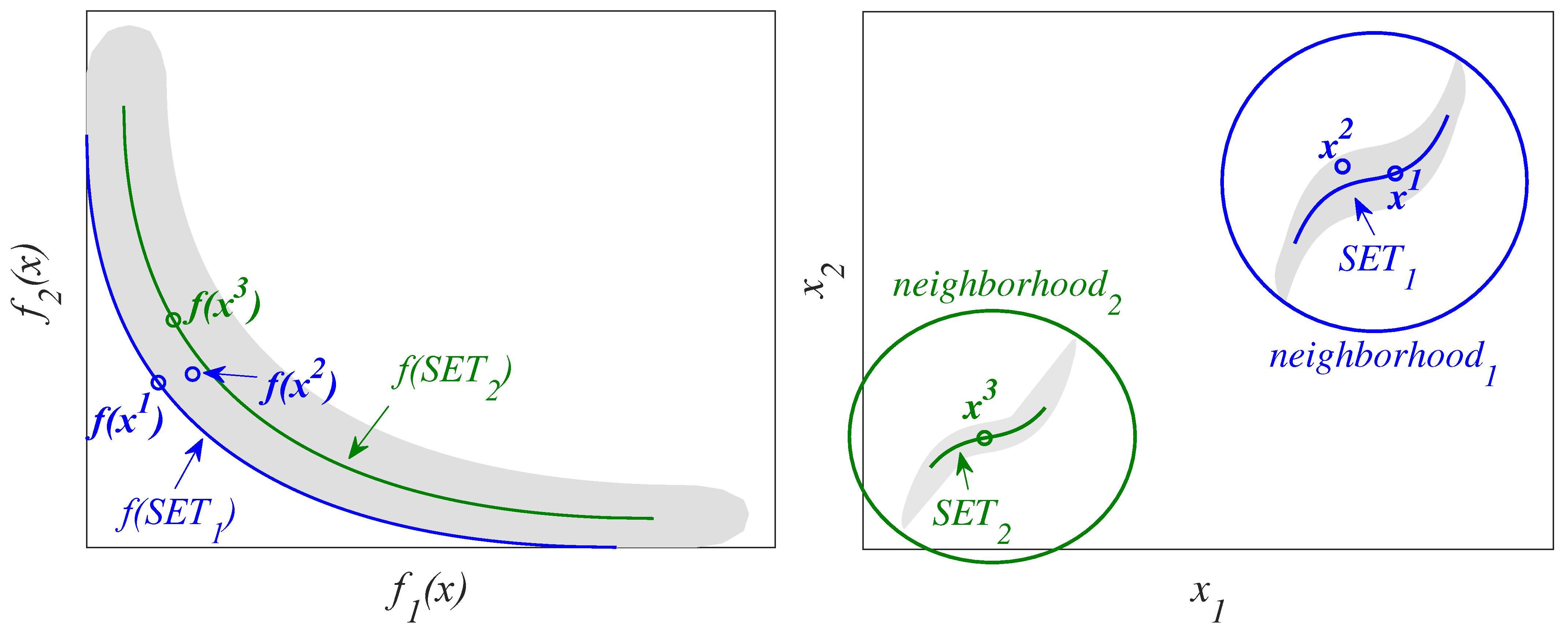
As discussed in the previous section, obtaining all nearly optimal solutions leads to problems. Considering only the most relevant solutions largely avoids the problems mentioned above. Not all nearly optimal solutions are equally useful to the DM. Therefore, if we manage to discard those that are less useful, we will reduce both mentioned problems. Let us see a graphic example to illustrate what we consider as potentially useful solutions. Suppose we have a MOOP with two design objectives and two decision variables (see Figure 1). Three solutions ${\mathit{x}}^{\mathbf{1}}$, ${\mathit{x}}^{\mathbf{2}}$ and ${\mathit{x}}^{\mathbf{3}}$ are selected. ${\mathit{x}}^{\mathbf{1}}$ is an optimal solution (member of the Pareto set), and it slightly dominates the nearly optimal solutions ${\mathit{x}}^{\mathbf{2}}$ and ${\mathit{x}}^{\mathbf{3}}$. ${\mathit{x}}^{\mathbf{1}}$ and ${\mathit{x}}^{\mathbf{2}}$ are very similar alternatives in their parameters (both belong to $neighborhoo{d}_1$, the same area in the parameter space), while ${\mathit{x}}^{\mathbf{3}}$ is significantly different (it belongs to $neighborhoo{d}_2$). In this scenario, ${\mathit{x}}^{\mathbf{2}}$ does not provide new relevant information to the DM. This solution is similar to ${\mathit{x}}^{\mathbf{1}}$ but with a worse performance in design objectives. Predictably, both will have similar characteristics, therefore the DM will choose ${\mathit{x}}^{\mathbf{1}}$ since it obtains a better performance in the design objectives. However, ${\mathit{x}}^{\mathbf{3}}$ does provide useful new information to the DM because it has a similar performance to the optimal ones and is in a different neighborhood. The solutions in $neighborhoo{d}_1$ could be, for example, not very robust or not feasible in practice. In this context, ${\mathit{x}}^{\mathbf{3}}$ (and the solutions in $neighborhoo{d}_2$) could be a potentially useful solution due to their significantly different characteristics. It is possible, and often common, for the DM to analyze in the decision stage additional indicators/objectives not included in the optimization phase. Thus, the DM can assume a small loss of performance in the design objectives in exchange for an improvement in a new feature not contemplated in the optimization process. This analysis can decide the final choice in one way or another. In short, including solutions of $neighborhoo{d}_2$ increases the diversity with useful solutions and enables the DM to make a better-informed final decision.

Therefore, the potentially useful nearly optimal solutions are those nearly optimal alternatives that differ significantly in the parameter space [28,29,30]. Thus, the new set must: (1) not neglect the diversity existing in the set of nearly optimal alternatives; (2) obtain the least number of solutions. To achieve both aims, it is necessary to employ an evolutionary algorithm that characterizes the set of solutions by means of a discretization which takes into account both the decision space and the objective space, simultaneously. A discretization that takes into account only the objective space can lead to the loss of significantly different nearly optimal alternatives in the decision space. This loss is a drawback because, as we have previously discussed, these alternatives are potentially useful. On the other hand, a discretization that takes into account only the decision space can lead to archives with a huge number of solutions [19] and cause the two problems previously mentioned.

3. Background

A multi-objective optimization problem can be defined as follows:

$$\begin{array}{c}\hfill \underset{\mathit{x}\in Q}{min}\mathit{f}\left(\mathit{x}\right)\end{array}$$

(1)

where $\mathit{x}=[x_1,...,x_k]$ is defined as a decision vector in the domain $Q \subset {\Re }^k$ and $\mathit{f}$: $Q\to {\Re }^m$ is defined as the vector of objective functions $\mathit{f}\left(\mathit{x}\right)=[f_1\left(\mathit{x}\right),...,f_m\left(\mathit{x}\right)]$. A maximization problem can be converted into a minimization problem. For each objective to be maximized $max{f}_i\left(\mathit{x}\right)=-min(-f_i\left(\mathit{x}\right))$ will be performed. The domain Q is defined by the set of constraints on $\mathit{x}$. For instance (but not limited to –any other constraints could be introduced in a general MOOP–):

$$\underline{x_i}\le x_i\le \overline{x_i}, i=[1,...,k]$$

(2)

where $\underline{x_i}$ and $\overline{x_i}$ are the lower and upper bounds of $\mathit{x}$ components.

Consequently, the MOOP obtains a Pareto set $P_Q$ (see Definition 2). This set has solutions non-dominated by any other solution (see Definition 1) in Q.

Definition 1

(Dominance [31]). A decision vector ${\mathit{x}}^{\mathbf{1}}$ is dominated by another decision vector ${\mathit{x}}^{\mathbf{2}}$ if $f_i\left({\mathit{x}}^{\mathbf{2}}\right)\le f_i\left({\mathit{x}}^{\mathbf{1}}\right)$ for all $i\in [1,...,m]$ and $f_j\left({\mathit{x}}^{\mathbf{2}}\right)<f_j\left({\mathit{x}}^{\mathbf{1}}\right)$ for at least one j, $j\in [1,...,m]$. This is denoted as ${\mathit{x}}^{\mathbf{2}}⪯{\mathit{x}}^{\mathbf{1}}$.

Definition 2.

(Pareto set $P_Q$): is the set of solutions in Q that is non-dominated by any other solution in Q: $P_Q:=\{\mathit{x}\in Q|\nexists {\mathit{x}}^{\prime }\in Q:{\mathit{x}}^{{}^{\prime }}⪯\mathit{x}\}$

Definition 3.

(Pareto front $\mathit{f}\left(P_Q\right)$): given a set of Pareto optimal solutions $P_Q$, the Pareto front is defined as:

$$\mathit{f}\left(P_Q\right):=\left\{\mathit{f}\left(\mathit{x}\right)\right|\mathit{x}\in P_Q\}$$

In any MOOP, there is a set of solutions with objective values close to the Pareto front. These solutions receive several names in the bibliography: nearly optimal, approximate, or $ϵ$-efficient solutions. To formalize the treatment of the nearly optimal solutions, the following definitions are used:

Definition 4.

($-ϵ$-dominance [32]): define $ϵ=[{ϵ}_1,...,{ϵ}_m]$ as the maximum acceptable degradation. A decision vector ${\mathit{x}}^{\mathbf{1}}$ is $-ϵ$-dominated by another decision vector ${\mathit{x}}^{\mathbf{2}}$ if $f_i\left({\mathit{x}}^{\mathbf{2}}\right)+{ϵ}_i\le f_i\left({\mathit{x}}^{\mathbf{1}}\right)$ for all $i\in [1,...,m]$ and $f_j\left({\mathit{x}}^{\mathbf{2}}\right)+{ϵ}_j<f_j\left({\mathit{x}}^{\mathbf{1}}\right)$ for at least one j, $j\in [1,...,m]$. This is denoted by ${\mathit{x}}^{\mathbf{2}}{⪯}_{-ϵ}{\mathit{x}}^{\mathbf{1}}$.

Definition 5.

(Set of nearly optimal solutions, $P_{Q,ϵ}$ [30]): is the set of solutions in Q which are not $-ϵ$-dominated by another solution in Q:

$$P_{Q,ϵ}:=\{\mathit{x}\in Q|\nexists {\mathit{x}}^{{}^{\prime }}\in Q:{\mathit{x}}^{{}^{\prime }}{⪯}_{-ϵ}\mathit{x}\}$$

The sets defined $P_Q$ and $P_{Q,ϵ}$ usually contain a great, or even infinite, number of solutions. Optimization algorithms try to characterize these sets using a discrete approximation $P_Q^{*}$ and $P_{Q,ϵ}^{*}$. In general, if such an approach has a limited set of solutions, the computational cost falls. However, the number of solutions must be sufficient to obtain a good characterization of these sets.

To compare the archiving strategies, it is useful to use a metric. Different metrics are used in the literature to measure the convergence of the outcome set. An example of these is the Hausdorff distance ($d_H$ [33,34,35] see Equation (3)).

$$\begin{array}{cc}\hfill d_H(A,B):& =max\left(dist\right(A,B),dist(B,A\left)\right)\hfill \\ \hfill dist(A,B):& =\underset{u\in A}{sup}dist(u,B)\hfill \\ \hfill dist(u,B):& =\underset{v\in B}{inf}\left|\right|u-v\left|\right|\hfill \end{array}$$

(3)

This metric is a measure of the distance between two sets. Therefore, $d_H$ can be used to measure convergence between the outcome set (or final archive) $f\left(A\right)$ to the target set $f\left(H\right)$ of a given MOOP (or archiving strategy). However, $d_H$ only penalizes the largest outlier of the candidate set. Thus, a high value of $d_H(A,H)$ can indicate both that A is a bad approximation of H and that A is a good approximation but contains at least one outlier. The $d_H$ is used by the archiver $ArchiveUpdate{P}_{Q,ϵ}{D}_{xy}$.

To avoid this problem, a new indicator appears in the literature: the averaged Hausdorff distance ${\Delta }_p$ (the standard Hausdorff distance is recoverable from ${\Delta }_p$ by taking the limit ${lim}_{p\to \infty }{\Delta }_p=d_H$). This metric (with $1\le p<\infty$) assigns a lower value to sets uniformly distributed throughout its domain. ${\Delta }_p$ is based on the known generational distance metrics (GD [36] and represents how “far” $f\left(H\right)$ is from $f\left(A\right)$), and inverted generational distance (IGD [37] represents how “far” $f\left(A\right)$ is from $f\left(H\right)$). However, these metrics are slightly modified in ${\Delta }_p$ ($G{D}_p$ and $IG{D}_p$, see Equation (5)). This modification means that the larger archive sizes and finer discretizations of the target set do not automatically lead to better approximations under ${\Delta }_p$ [34]. ${\Delta }_p$ measures the diversity and convergence in the decision and objective spaces. In this work we use ${\Delta }_p$ with $p=2$ (as in [18,38]) so that the influence of outliers is low.

$$\begin{array}{c}\hfill {\Delta }_p(X,Y):=max(G{D}_p(X,Y),IG{D}_p(X,Y))\end{array}$$

(4)

where

$$\begin{array}{cc}\hfill G{D}_p& ={\left(\frac{1}{n_x}\sum _{i=1}^{n_x}dist{(x_i,Y)}^p\right)}^{1/p}\hfill \\ \hfill IG{D}_p& ={\left(\frac{1}{n_y}\sum _{i=1}^{n_y}dist{(y_i,X)}^p\right)}^{1/p}\hfill \end{array}$$

(5)

where

$$\begin{array}{c}\hfill dist(u,A):=\underset{v \in A}{inf}\left|\right|u-v\left|\right|\end{array}$$

(6)

To use ${\Delta }_p$ it is necessary to define the target set H with which to compare the final archive A obtained by the archivers. The target set is defined in the decision space (H) and it has its representation in the objective space ($f\left(H\right)$). The definition of H is possible on the benchmarks used in this work (where the global and local optimum are known), but this definition is not trivial. $Archive\_nevMOGA$ and $ArchiveUpdate{P}_{Q,ϵ}{D}_{xy}$ archivers discard solutions similar in both spaces at the same time. However, $Archive$- $\_nevMOGA$, unlike $ArchiveUpdate{P}_{Q,ϵ}{D}_{xy}$, discards dominated solutions in their neighborhood. $targetSelect$ looks for diversity in both spaces simultaneously. On the one hand, defining H as the optimal and nearly optimal solutions that are not similar in both spaces at the same time, would give the archive $ArchiveUpdate{P}_{Q,ϵ}{D}_{xy}$ an advantage. If H is defined as the set of optimal and nearly optimal solutions non-dominated in their neighborhood, $Archive\_nevMOGA$ would be benefited. However, the archivers have a common goal: to obtain the solutions close to the optimals in the objective space but significantly different in the decision space (potentially useful solutions). Consequently, to be as “fair” as possible we must define H as the set that defines the common objective. Thus, the potentially useful solutions can be represented by the local Pareto set (see Definition 6).

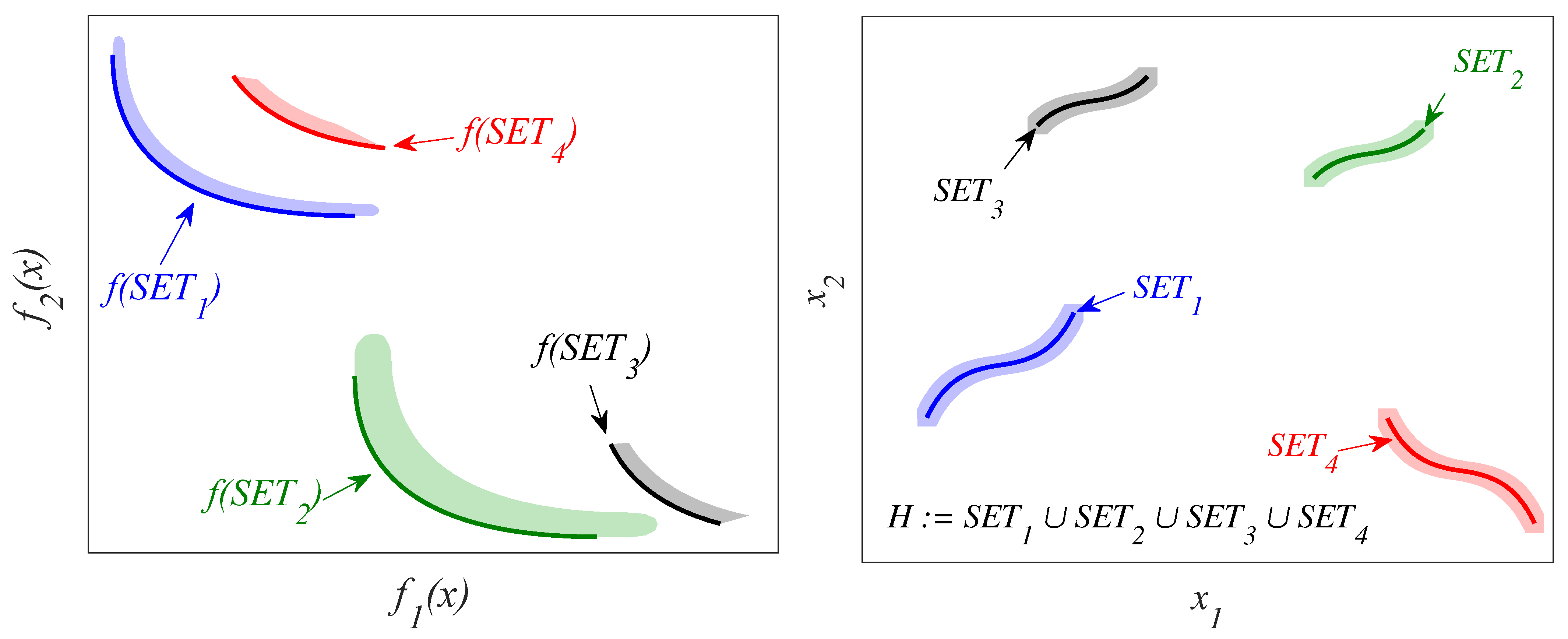
Definition 6.

(Local Pareto set [5,39]): is the set of solutions in Q that is non-dominated by any another neighbor solution in Q (where n is a small positive number):

$$H:=\{x\in Q|\nexists y\in Q: \left|\right|x-y|{|}_{\infty }\le n and y⪯x\}$$

Figure 2 shows an example of a MOOP with two design objectives and two decision variables. Sets $SE{T}_1$ and $SE{T}_2$ form the global Pareto set. Both sets, together with $SE{T}_3$ and $SE{T}_4$ form the local Pareto set (since the global Pareto set is also a local Pareto set). No solution of a local Pareto set is dominated by a neighboring solution. Furthermore, all the solutions neighboring the local Pareto set are dominated by a neighboring solution, and therefore they are not part of this set. This can be verified by the colored areas around the sets $SE{T}_1$, $SE{T}_2$, $SE{T}_3$ and $SE{T}_4$. For example, solutions in the gray area, which are neighboring solutions to $SE{T}_3$, obtain a worse objective value than $SE{T}_3$. For this reason, the solutions of the gray area are dominated by neighboring solutions, and therefore are not part of the local Pareto set. Sets $SE{T}_3$ and $SE{T}_4$ provide the DM with alternatives potentially useful (significantly different to $SE{T}_1$ and $SE{T}_2$), enabling the DM to make a more informed final decision. For this work, the $ϵ-$dominated solutions (solutions that are not in the set $P_{Q,ϵ}$) will not be considered to be local Pareto solutions (H) because their degradation in performance is significant for the DM.

4. Description of the Compared Archivers

As already discussed above, nearly optimal solutions can be very useful. However, it is necessary to discretize this set in order to find a reduced set of solutions to avoid the problems associated with an excessive number of solutions. Furthermore, it is necessary not to neglect the potentially useful nearly optimal solutions, i.e., nearly optimal alternatives significantly different (in the decision space) to the optimal solutions. To achieve both purposes, it is essential to discretize the set of solutions taking into account the decision and objective spaces at the same time. In this section, three archivers that discretize the set $P_{Q,ϵ}$ in both spaces are described.

There are MMEAs and algorithms that consider nearly optimal solutions that offer these solutions: $P_{Q,ϵ}$-NSGA-II [28], $P_{Q,ϵ}$-MOEA [30], nevMOGA [29], N$ϵ$SGA [18], DIOP [10], 4D-Miner [40,41], MNCA [42].

$P_{Q,ϵ}$-NSGA-II [28] was one of the first algorithms aimed at finding approximate (nearly optimal) solutions. $P_{Q,ϵ}$-NSGA-II uses the same classification strategy as the algorithm on which it is based, NSGA-II [43], and therefore, the highest pressure of the population is taken toward the Pareto set. Thus, this may result in the neighborhoods with only nearly optimal solutions not being adequately explored [30]. To avoid this problem, the algorithm $P_{Q,ϵ}$-MOEA [30] is created. This algorithm was designed to avoid Pareto set bias. Nevertheless, $P_{Q,ϵ}$-MOEA does not take into account the location of solutions in the decision space. $P_{Q,ϵ}$-MOEA does not then guarantee that the potentially useful alternatives will not be discarded. To overcome this problem, the nevMOGA [29] algorithm was designed. This algorithm seeks to ensure that the potentially useful alternatives are not discarded. DIOP [10] is a set-based algorithm that can maintain dominated solutions. This algorithm simultaneously evolves two populations A and T. Population A approaches the Pareto front, and is not provided to the DM, while T is the target population that seeks to maximize diversity in the decision and objective spaces. MNCA [42] is an evolutive algorithm that simultaneously evolves multiple subpopulations. In MNCA each subpopulation converges to a different set of non-dominated solutions. Finally, 4D-Miner [40,41] is an algorithm especially designed for functional brain imaging problems.

One of the crucial points in an evolutionary multi-objective optimization algorithm is the archiving strategy. The $P_{Q,ϵ}$-NSGA-II and $P_{Q,ϵ}$-MOEA algorithms share the $ArchiveUpdate{P}_{Q,ϵ}$ archiver. This archiver seeks to characterize all nearly optimal solutions without taking into account the decision space. In [19], different archiving strategies are compared: $ArchiveUpdate{P}_{Q,ϵ}$, $ArchiveUpdate{P}_{Q,ϵ}{D}_x$, $ArchiveUpdate{P}_{Q,ϵ}{D}_y$ and $ArchiveUpdate{P}_{Q,ϵ}{D}_{xy}$. On the one hand, $ArchiveUpdate{P}_{Q,ϵ}$ gets an excessive number of solutions. On the other hand, $ArchiveUpdate{P}_{Q,ϵ}{D}_x$, $ArchiveUpdate{P}_{Q,ϵ}{D}_y$ do not discretize the decision and objective spaces simultaneously. Therefore, these archivers do not achieve the two purposes discussed above. The mentioned work concludes that archiver $ArchiveUpdate{P}_{Q,ϵ}{D}_{xy}$ is most practical use within stochastic search algorithms. Furthermore, this archiver is the only one of the archivers compared in this paper that discretizes the decision and objective spaces simultaneously [27], a factor that we consider necessary to obtain potentially useful solutions. The archiver $ArchiveUpdate{P}_{Q,ϵ}{D}_{xy}$ has been employed in the recent N$ϵ$SGA algorithm to maintain a well-distributed representation in the decision and objective spaces. For this reason, the present work compares the archiver $ArchiveUpdate{P}_{Q,ϵ}{D}_{xy}$ and not $ArchiveUpdate{P}_{Q,ϵ}$, $ArchiveUpdate{P}_{Q,ϵ}{D}_x$ and $ArchiveUpdate{P}_{Q,ϵ}{D}_y$.

The second archiver included in this comparison is the archiver of the nevMOGA algorithm ($Archive\_nevMOGA$). This archiver characterizes the set of potentially useful solutions by discretizing both spaces simultaneously. Finally, the archiver of the DIOP algorithm ($targetSelect$) is also compared in this work. $targetSelect$ seeks to find the population that maximizes an indicator that measures diversity in the decision and objective spaces simultaneously. Therefore, a metric-based archiver $targetSelect$ is compared to the distance-based archivers $ArchiveUpdate{P}_{Q,ϵ}{D}_{xy}$ and $Archive\_nevMOGA$. The three archivers compared in this work seek to characterize the potentially useful solutions. The archiver of the MNCA algorithm has not been included in the comparison because it looks for non-dominated solutions. The archiver of the 4D-Miner algorithm has also not been included in the comparison because 4D-Miner is a very specific algorithm for functional brain imaging problems.

4.1. $ArchiveUpdate{P}_{Q,ϵ}{D}_{xy}$

$ArchiveUpdate{P}_{Q,ϵ}{D}_{xy}$ is the proposed archiving strategy in [19] (see Algorithm 1). As already mentioned, potentially useful solutions are those that obtain similar performance (in the design objectives) but differ significantly in their parameters (in the decision space). This archiver aims to maintain these solutions. This archiver uses, in addition to the parameter $ϵ$ (maximum degradation acceptable to the DM, see Definition 4), the parameters ${\Delta }_x$ and ${\Delta }_y$. Two solutions are considered similar if their distance in the decision space is less than ${\Delta }_x$. Therefore, the parameter ${\Delta }_x$ is the maximum distance, in the decision space, between two similar solutions. Two alternative solutions obtain a similar performance if their distance in the objective space is less than ${\Delta }_y$. Therefore, the parameter ${\Delta }_y$ is the maximum distance between two solutions to be considered similar in the objectives space. Both parameters are measured using the Hausdorff distance [34] ($d_H$, see Equation (3)). The archive A stores the set of obtained alternatives. A new solution p from P (new candidate solutions) will only be incorporated in A if: (1) p is a nearly optimal solution; and (2) A does not contain any solution similar to p, in the decision and objective spaces at the same time. If the new solution p is stored in archive A, the new set of optimal and nearly optimal solutions ($\widehat{A}$) belonging to archive A is calculated. Thus, a solution $a\in A$ will be removed if: (1) it is not a nearly optimal solution ($p{\prec }_{-(ϵ+{\Delta }_y)}a$); and (2) the distance to the set $\widehat{A}$ fulfills the condition $dist(a,\widehat{A})\ge 2{\Delta }_x$.

Algorithm 1$A:=ArchiveUpdate{P}_{Q,ϵ}{D}_{xy}(P,A_0,ϵ,{\Delta }_x,{\Delta }_y)$

Require: population P, archive $A_0,ϵ\in {\mathbb{R}}_{+}^m,{\Delta }_x\in {\mathbb{R}}_{+},{\Delta }_y\in {\mathbb{R}}_{+}$

Ensure: update archive A

1: $A:=A_0$ 2: for all$p\in P$do 3:   if $(\nexists a_1\in A:a_1{\prec }_{-ϵ}p)$ and $(\nexists a_2:(d_H(f\left(a_2\right),f\left(p\right))\le {\Delta }_y$ and $d_H(a_2,p)\le {\Delta }_x\left)\right)$ then 4:     $A\leftarrow A\cup \left\{p\right\}$ 5:     $\widehat{A}=\{a_1\in A|\nexists a_2\in A:a_2{\prec }_{-(ϵ+{\Delta }_y)}{a}_1\}$ 6:     for all $a\in A$ \ $\widehat{A}$ do 7:      if $p{\prec }_{-(ϵ+{\Delta }_y)}a$ and $dist(a,\widehat{A})\ge 2{\Delta }_x$ then 8:       $A\leftarrow A$ \ {a} 9:      end if 10:     end if 11:   end if 12: end if

The archiver $ArchiveUpdate{P}_{Q,ϵ}{D}_{xy}$ goes through all the set of candidate solutions $p\in P$, and in the worst case, the algorithm compares them with all the solutions $a\in A$. Thus, the complexity of the archiver is $O\left(\right|P\left|\right|A\left|\right)$ [44]. Also, $ArchiveUpdate{P}_{Q,ϵ}{D}_{xy}$ has a maximum number of solutions $\left|A\right(D_{xy}\left)\right|$ [19] which is given by:

$$|A\left(D_{xy}\right)|\le |A\left(D_{xy}^x\right)\left|\right|A\left(D_{xy}^y\right)|$$

(7)

where $\left|A\right(D_{xy}^x\left)\right|$ is the maximum number of neighborhoods that the decision space can contain (based on ${\Delta }_x$) and $\left|A\right(D_{xy}^y\left)\right|$ is the maximum number of solutions that can exist in each neighborhood (based on ${\Delta }_y$ and $ϵ$), and are defined as:

$$|A\left(D_{xy}^x\right)|\le \prod _{i=1}^k\left(\frac{1}{{\Delta }_x}+1\right)\prod _{j=1}^k(\overline{x_j}-\underline{x_j})$$

(8)

$$|A\left(D_{xy}^y\right)|\le {\left(\frac{1}{{\Delta }_y}\right)}^{m-1}\sum _{i=1}^m\left(\frac{{ϵ}_i}{{\Delta }_y}+3\right)\prod _{\begin{array}{c}i=1\\ i\ne j\end{array}}^m(M_j-m_j+{\Delta }_y)$$

(9)

$\underline{x_j}$ and $\overline{x_j}$ are the bounds in the decision space ($P_{Q,ϵ+2{\Delta }_y}$ is included in $[\underline{x_1},\overline{x_1}]\dots [\underline{x_k},\overline{x_k}]$) and $M_j$ and $m_j$ are the bounds in the objective space of the set to discretize $f\left(P_{Q,ϵ+2{\Delta }_y}\right)$. Also, it is assumed that any ${ϵ}_i$ is greater than ${\Delta }_y$.

4.2. $Archive\_nevMOGA$

$Archive\_nevMOGA$ is the archiving strategy used by the nevMOGA evolutionary algorithm [29]. This archiver, just as $ArchiveUpdate{P}_{Q,ϵ}{D}_{xy}$, aims to guarantee solutions that obtain similar performance to the optimals, but are significantly different in the decision space. The archiver $Archive\_nevMOGA$ uses the same three parameters as $ArchiveUpdate{P}_{Q,ϵ}{D}_{xy}$ ($ϵ$, ${\Delta }_x$, ${\Delta }_y$). However, there are differences in the definition of some parameters in this archiver with respect to $ArchiveUpdate{P}_{Q,ϵ}{D}_{xy}$: (1) ${\Delta }_{\mathit{x}}$ is a vector that contains the maximum distances (in the decision space) between similar solutions for each dimension. Thus, two individuals a and b are similar if: $|a_i-b_i|\le {\Delta }_{x_i} \forall i\in [1,\dots ,k]$. (2) ${\Delta }_{\mathit{y}}$ is also a vector that contains the maximum distances (in the objective space) between solutions with similar performance for each dimension. Thus, two individuals a and b have a similar performance if: $|f_i\left(a\right)-f_i\left(b\right)|\le {\Delta }_{y_i} \forall i\in [1,\dots ,m]$.

The archiver $Archive\_nevMOGA$ will add a new candidate solution p to the archive A if the following conditions are met simultaneously: (1) p is a nearly optimal solution; (2) there is no similar solution to p (in the decision space) $\in A$ that dominates it; and (3) there is no similar solution to p in A in both spaces at the same time (if it exists, and p dominates it, it will be replaced). If a solution p is incorporated in the archive A, it will remove from A: (1) the similar individuals (in the parameter space) that are dominated by p and (2) the individuals $ϵ-$dominated by p.

The complexity of the archiver $Archive\_nevMOGA$ is equivalent to the complexity of $ArchiveUpdate{P}_{Q,ϵ}{D}_{xy}$ previously defined ($O\left(\right|P\left|\right|A\left|\right)$). Moreover, $Archive\_nevMOGA$ has a maximum number of solutions $\left|A\right(nMOGA\left)\right|$ which is given by:

$$\left|A\left(nMOGA\right)\right|\le |A\left(nMOG{A}^x\right)\left|\right|A\left(nMOG{A}^y\right)|$$

(10)

where ${\left|A\left(nMOGA\right)\right|}^x$ is the maximum number of neighborhoods that the decision space can contain (based on ${\Delta }_{\mathit{x}}$) and ${\left|A\left(nMOGA\right)\right|}^y$ is the maximum number of solutions that can exist in each neighborhood (based on ${\Delta }_{\mathit{y}}$ and $ϵ$), and are defined as:

$$|A\left(nMOG{A}^x\right)|\le \prod _{i=1}^k\left(\frac{1}{{\Delta }_{x_i}}+1\right)\prod _{j=1}^k(\overline{x_j}-\underline{x_j})$$

(11)

$$|A\left(nMOG{A}^y\right)|\le \frac{{\prod }_{i=1}^{m}n\_bo{x}_i}{n\_bo{x}_{max}}$$

(12)

where $n\_bo{x}_i=(M_i-m_i)/{\Delta }_{y_i}$, $n\_bo{x}_{max}={max}_{i}n\_bo{x}_i$ and $M_j$ and $m_j$ are the bounds in the objective space of the set to discretize $f\left(P_{Q,ϵ}\right)$.

The archive size with respect to the decision space is equivalent for the compared archivers ($A\left(D_{xy}^x\right)$ and $A\left(nMOG{A}^x\right)$). However, there is a difference between $A\left(D_{xy}^y\right)$ and $A\left(nMOG{A}^y\right)$ (objective space). The archiver $Archive\_nevMOGA$, unlike $ArchiveUpdate{P}_{Q,ϵ}{D}_{xy}$, discards nearly optimal solutions dominated by a similar solution in the decision space. Thus, in the worst case, $Archive\_nevMOGA$ will obtain the best solutions (non-dominated) in each neighborhood. These solutions will have a maximum number of alternatives depending on ${\Delta }_{\mathit{y}}$. However, $ArchiveUpdate{P}_{Q,ϵ}{D}_{xy}$, in the worst case, will obtain, in each neighborhood, in addition to the best solutions, additional solutions. These additional solutions are dominated by neighboring solutions, but are considered solutions with different performance (based on ${\Delta }_y$). As a result, the archive of $Archive\_nevMOGA$ will have fewer solutions than the archive of $ArchiveUpdate{P}_{Q,ϵ}{D}_{xy}$. Therefore, we can deduce that the archiver $Archive\_nevMOGA$ has a lower computational cost than $ArchiveUpdate{P}_{Q,ϵ}{D}_{xy}$ because its archive contains fewer solutions (the candidate solutions are compared with a smaller number of solutions).

4.3. $targetSelect$

$targetSelect$ is the archiving strategy used by the DIOP evolutionary algorithm [10]. This archiver seeks to obtain a diverse set of solutions (keeping solutions close to the Pareto set) in the decision and objective spaces. $A=targetSelect(F,T,{\mu }^t,ϵ)$ has as inputs: an approximation to the Pareto front F, the set of solutions to be analyzed T, the size of the set target ${\mu }^t$, and $ϵ$. This archiver selects ${\mu }^t$ solutions from set T. The goal is to find the population A, with size ${\mu }^t$, to maximize $G\left(T\right)$ (see Equation (13)). $G\left(T\right)$ is defined as the sum of the product between a metric and its respective weight.

$$G\left(T\right):={\omega }_o·D_o\left(T\right)+{\omega }_d·D_d\left(T\right),\left|T\right|=\mu \mathrm{with}{q}_F\left(t\right)\le ϵ \forall t\in T,{\omega }_o+{\omega }_d=1$$

(13)

where $D_o$ and $D_d$ are metrics that measure diversity in the objective and decision spaces respectively, and $q_F$ is a distance metric defined as:

$$q_F\left(x\right):=min\{ϵ | \exists y\in F:x{⪯}_{ϵ}y\}$$

(14)

$D_o$ is an indicator that measures diversity and convergence to the Pareto front, and $D_d$ is an indicator that measures diversity in the decision space. In this work, as in [10], $D_o$ and $D_d$ were specified by the hypervolume indicator [45] and the Solow–Polasky diversity measure [46], respectively. An advantage of the archiver $targetSelect$ is that you can directly and arbitrarily specify the archive size.

5. Materials and Methods

In this section, the MOOPs, on which the three archivers will be compared, will be defined. In addition, the methodology for carrying out the comparison is introduced.

5.1. Definition of MOOPs

The archivers will be compared on two benchmarks and a real engineering example. Benchmarks have a very low computational cost for the objective function. For this reason, it is inexpensive to obtain a target set (with a very fine discretization in the decision space) H. This discrete set is necessary for the use of the metric ${\Delta }_p$ (see Section 3). Furthermore, the definition of this set must be as “fair” as possible. Therefore, for the benchmarks, the target set H is defined as the local and global Pareto set (see justification in Section 3). This set is obtained by discretizing the decision space with 10,000,000 solutions in the range of the parameters. Furthermore, the target set H has its representation in the objective space. In the real engineering example, obtaining a set H would be computationally very expensive (or even unaffordable). Therefore, this set is not defined in this MOOP. By means of these problems it is possible to analyze the behavior of the archivers for different characteristics in the MOOP: multimodal solutions; local Pareto sets; or discontinuous Pareto fronts. However, there are other features of MOPs that are not analyzed in this article (such as MOPs with many objectives and/or decision variables).

5.1.1. Benchmark 1

Benchmark 1 (see Equation (15)) is a test problem called SYM-PART defined in [47] widely used in the literature [18,20,48,49,50] for the evaluation of algorithms that characterize nearly optimal or multimodal solutions. Benchmark 1 has the Pareto set located in a single neighborhood, and it also has eight local Pareto set that overlap in the objective space (see Equation (20) and Figure 3). Thus, this benchmark is very useful to observe if the compared archivers can adequately characterize the nine existing neighborhoods, and provide all the existing diversity to the DM.

$$\begin{array}{c}\hfill \begin{array}{c}\\ min\\ \mathit{x}\end{array} \mathit{f}\left(\mathit{x}\right)=[f_1\left(\mathit{x}\right) f_2\left(\mathit{x}\right)]\end{array}$$

(15)

$$\begin{array}{c}\hfill f_1\left(\mathit{x}\right)={(x_1-t_1(c+2a)+a)}^2+{(x_2-t_{2}b)}^2+{\delta }_t\\ \hfill f_2\left(\mathit{x}\right)={(x_1-t_1(c+2a)-a)}^2+{(x_2-t_{2}b)}^2+{\delta }_t\end{array}$$

(16)

where

$$t_1=sgn\left(x_1\right)min\left(⌈\frac{|x_1|-a-c/2}{2a+c}⌉,1\right)$$

$$t_2=sgn\left(x_2\right)min\left(⌈\frac{|x_2|-b/2}{b}⌉,1\right)$$

and

$${\delta }_t=\left\{\begin{array}{cc}0\hfill & for t_1=0 and t_2=0\hfill \\ 0.1\hfill & else\hfill \end{array}\right.$$

subject to:

$$\begin{array}{c}\hfill -20\le x_1\le 20\\ \hfill -20\le x_2\le 20\end{array}$$

(17)

using $a=0.5$, $b=5$ and $c=5$.

This MOOP contains one global Pareto set:

$$\begin{array}{c}\hfill P_{0,0}=[-0.5,0.5]\times \left\{0\right\}=P_Q\end{array}$$

(18)

as well as the following eight local Pareto sets:

$$\begin{array}{c}\hfill \left.\begin{array}{cc}{P}_{-1,-1}& =[-6.5,-5.5]\times \{-5\}\\ P_{0,-1}& =[-0.5,0.5]\times \{-5\}\\ P_{1,-1}& =[5.5,6.5]\times \{-5\}\\ P_{-1,0}& =[-6.5,-5.5]\times \left\{0\right\}\\ P_{1,0}& =[5.5,6.5]\times \left\{0\right\}\\ P_{-1,1}& =[-6.5,-5.5]\times \left\{5\right\}\\ P_{0,1}& =[-0.5,0.5]\times \left\{5\right\}\\ P_{1,1}& =[5.5,6.5]\times \left\{5\right\}\end{array}\right\}Local Pareto set\end{array}$$

(19)

Therefore, the target set H is defined as:

$$\begin{array}{cc}\hfill H& :=P_{0,0}\cup P_{-1,-1}\cup P_{0,-1}\cup P_{1,-1}\cup P_{-1,0}\cup P_{1,0}\cup P_{-1,1}\cup P_{0,1}\cup P_{1,1}\hfill \end{array}$$

(20)

To evaluate the archivers on benchmark 1, the parameters are defined in

Table 1. Parameters for benchmark 1.

Parameters	Value
$ϵ$	$[0.15 0.15]$
$ArchiveUpdate{P}_{Q,ϵ}{D}_{xy}$
${\Delta }_x$	1
${\Delta }_y$	$0.2$
$Archive\_nevMOGA$
${\Delta }_{\mathit{x}}$	$[1 1]$
${\Delta }_{\mathit{y}}$	$[0.2 0.2]$
$targetSelect$
${\mu }^t$	100
${\omega }_o$	$0.9677$ (uniform dispersion)
${\omega }_o$	$0.7692$ (random dispersion)

. The parameters $ϵ$, ${\Delta }_x$ and ${\Delta }_y$ are defined based on prior knowledge of the problem. The $targetSelect$ archiver is based on an indicator, and therefore has different parameters from the rest of the compared archives. For the choice of the parameter ${\mu }^t$, based on the size of the archives obtained by the rest of the archivers, the following values have been analyzed: ${\mu }^t=\{100,75,50\}$. For the choice of the ${\omega }_o$ parameter, the following parameters suggested in [10] have been analyzed: ${\omega }_o=\{0,0.7692,0.9091,0.9677,1\}$. Among all these values, ${\mu }^t=100$ and ${\omega }_o=0.9677$ have been defined as the parameters that obtain the best performance, with respect to ${\Delta }_p$, for the uniform dispersion. For random dispersion, ${\omega }_o=0.7692$ obtain the best performance.

5.1.2. Benchmark 2

The benchmark 2 (see Equation (21)) is an adaptation of the modified Rastrigin benchmark [51,52,53,54]. Figure 4 show the global and local Pareto set H of benchmark 2. This benchmark has a discontinuous Pareto front made up of solutions in different neighborhoods. In addition, it also provides nearly optimal solutions significantly different from the optimal solutions (in different neighborhoods).

$$\begin{array}{c}\hfill \underset{\mathit{x}}{min}\mathit{f}\left(\mathit{x}\right)=[f_1\left(\mathit{x}\right) f_2\left(\mathit{x}\right)]\end{array}$$

(21)

$$\begin{array}{c}\hfill f_1\left(\mathit{x}\right)=-(\sum _{i=1}^{2}10+9cos(2\pi ·k_i·x_i))(1-\sqrt{{(x_1-0.65)}^2+{(x_2-0.5)}^2})\\ \hfill f_2\left(\mathit{x}\right)=min\left(\right(x_1-0.65)+(x_2-0.5),(x_1-0.65)+(x_2-0.25),(x_1-\\ \hfill 0.65)+(x_2-0.75),(x_1-0.35)+(x_2-0.5),(x_1-0.35)+(x_2-0.75),\\ (x_1-0.35)+(x_2-0.25))\end{array}$$

(22)

where $k_1=2$ and $k_2=3$, and subject to:

$$\begin{array}{c}\hfill 0\le x_1\le 4\\ \hfill 0\le x_2\le 4\end{array}$$

(23)

To analyze the archivers on the benchmark 2, we define the parameters of

Table 2. Parameters for benchmark 2.

Parameters	Value
$ϵ$	$[2.5 0.15]$
$ArchiveUpdate{P}_{Q,ϵ}{D}_{xy}$
${\Delta }_x$	$0.15$
${\Delta }_y$	$0.25$
$Archive\_nevMOGA$
${\Delta }_{\mathit{x}}$	$[0.15 0.15]$
${\Delta }_{\mathit{y}}$	$[0.25 0.25]$
$targetSelect$
${\mu }^t$	150
${\omega }_o$	$0.9677$ (uniform dispersion)
${\omega }_o$	$0.9091$ (random dispersion)

. The parameters $ϵ$, ${\Delta }_x$ and ${\Delta }_y$ are defined based on prior knowledge of the problem. Following the same procedure as the previous benchmark, ${\mu }^t=150$ (in this case ${\mu }^t=\{200,150,100\}$ has been analyzed) and ${\omega }_o=0.9677$ is defined as the parameters that obtains the best performance, with respect to ${\Delta }_p$, for the uniform dispersion. For random dispersion, ${\omega }_o=0.9091$ obtains the best performance.

5.1.3. Identification of a Thermal System

Finally, a MOOP is defined to solve a real engineering problem: identification of a thermal system. In this problem, the energy contribution inside the process is due to the power dissipated by the resistance inside it (see Figure 5). Air circulation inside the process is produced by a fan, which constantly introduces air from outside. The actuator is made up of a voltage source which is controlled by voltage. The actuator input range is $[0 100]$ % ($[0 7.5]$ V). Two thermocouples are used to measure the resistance temperature and the air temperature in the range $[-50 250]{}^{°}$C. Figure 6 shows the signals that will be used in the identification process. The ambient temperature $T_a$ is considered constant and equal to 17 ${}^{°}$C for the entire identification test.

Taking into account the physical laws of thermodynamics [55], the initial structure of the model can be defined using the following differential equations, where heat losses due to convection and conduction are modeled, as well as losses due to radiation:

$$\begin{array}{cc}\hfill & \dot{T}\left(t\right)=\frac{1}{1000}\left(x_{1}v{\left(t\right)}^2-x_2(T\left(t\right)-T_a\left(t\right))-x_3{\left(\frac{273.0+T\left(t\right)}{100}\right)}^4\right)\hfill \end{array}$$

(24)

where $T\left(t\right)$ is the process output temperature and state variable in ${}^{°}$C, $v\left(t\right)$ is the input voltage to the process in volts, $T_a\left(t\right)$ is the ambient temperature in ${}^{°}$C and $\mathbf{x}=[x_1 x_2 x_3]$ are the parameters of the model to estimate.

The MOOP is defined as follows:

$$\begin{array}{c}\hfill \underset{\mathit{x}}{min}\mathit{f}\left(\mathit{x}\right)=[f_1\left(\mathit{x}\right) f_2\left(\mathit{x}\right)]\end{array}$$

(25)

subject to:

$$\underline{\mathit{x}}\le \mathit{x}\le \overline{\mathit{x}}$$

where:

$$f_1=\frac{1}{\tau }{\int }_0^{\tau }|\widehat{T}-T|dt$$

(26)

$$f_2=\underset{i \in 1...\tau }{max}|\widehat{T_i}-T_i|$$

(27)

$\tau =2500$ is the duration of the identification test, variables with circumflex accent are process outputs (experimental data), variables without circumflex accent are the model outputs, $\mathit{x}$ the parameter vector:

$$\mathit{x}=[x_1 x_2 x_3]$$

(28)

and $\underline{\mathit{x}}$ and $\overline{\mathit{x}}$ (see

Table 3. Lower ($\underline{\mathit{x}}$) and upper ($\overline{\mathit{x}}$) limits of the parameters $\mathit{x}$.

Limits	${\mathit{\theta }}_1$	${\mathit{\theta }}_2$	${\mathit{\theta }}_3$
$\underline{\mathit{x}}$	0.01	2	0
$\overline{\mathit{x}}$	0.15	10	0.8

) the lower and upper limits of the parameter vector $\mathit{x}$ which define the decision space Q.

In this MOOP, the design objectives measure the mean and maximum error between the temperatures of the process outlet and the model. The parameters to be estimated and the design objectives have a physical meaning. This fact makes it easier to choose the $ϵ$, ${\Delta }_x$ and ${\Delta }_y$ (see

Table 4. Parameters for identification of thermal system.

Parameters	Value
$ϵ$	$[0.25 0.25]$
$ArchiveUpdate{P}_{Q,ϵ}{D}_{xy}$
${\Delta }_x$	$0.1$
${\Delta }_y$	$0.025$
$Archive\_nevMOGA$
${\Delta }_{\mathit{x}}$	$[0.0015 0.2 0.1]$
${\Delta }_{\mathit{y}}$	$[0.025 0.025]$
$targetSelect$
${\mu }^t$	78
${\omega }_o$	$0.7692$

). The $ϵ$ parameter (maximum acceptable degradation) is the same for all archivers. ${\Delta }_y$ is similar for $ArchiveUpdate{P}_{Q,ϵ}{D}_{xy}$ and $Archive\_nevMOGA$, taking into account the difference in vector size. However, ${\Delta }_x$ is different for $ArchiveUpdate{P}_{Q,ϵ}{D}_{xy}$ and $Archive\_nevMOGA$. For $ArchiveUpdate{P}_{Q,ϵ}{D}_{xy}$, ${\Delta }_x=0.1$. A lower value increases significantly higher number of solutions. A higher value gives a poor approximation to the set of optimal and nearly optimal solutions. For $Archive\_nevMOGA$, ${\Delta }_{\mathit{x}}=[0.0015 0.2 0.1]$. In this case, ${\Delta }_{\mathit{x}}$ is independent for each dimension in the decision space, being different for each parameter due to its different limits (see Table 3). For $targetSelect$, ${\mu }^t=78$ solutions to obtain the same number of solutions as $Archive\_nevMOGA$. In this way, both archivers will have equal conditions. Additionally, ${\omega }_o=0.7692$ is defined to give greater weight to diversity in the decision space.

5.2. Archivers Comparison Procedure

The procedure performed to carry out the archiver comparison is different on the benchmarks and on the real example. Benchmarks have a very low computational cost for the objective function. Therefore, it is possible to evaluate large populations that discretize the entire search space. These populations are entered in the archiver as input population. To analyze the behavior of the archivers on different types of populations, a uniform and random distribution is used to obtain these initial populations.

Because the computational cost of the objective functions of the engineering problem are significantly higher, it is not feasible to test each archiver with random or exhaustive searches as has been done with the benchmarks. Thus, the archiver has been embedded in a basic evolutionary algorithm. In addition to the reduction of computational cost, this enables observing the impact of each archiver when incorporated into an evolutionary mechanism.

5.2.1. Benchmarks

For the comparison of the archivers on the two benchmarks presented, the archivers will be fed in two ways: (1) by a uniform distribution; (2) by a random distribution of solutions in the search space. The comparison of the results will be made using the averaged Hausdorff distance ${\Delta }_p$ [34] (see Equation (4)). This metric measures the averaged Hausdorff distance between the outcome set (or final archive) $f\left(A\right)$ and the target set $f\left(H\right)$ (local Pareto set in this paper) of a given MOOP. Since ${\Delta }_p$ considers the averaged distances between the entries of $f\left(A\right)$ and $f\left(H\right)$, this indicator is very insensitive to outliers. This metric measures the diversity and convergence towards the target set. Furthermore, this metric can be applied both in the decision and objective space.

To carry out the comparison of the archiving strategies with data of a uniform dispersion, each archiver is fed with a file of 100,000 solutions uniformly distributed throughout the domain Q (generating a hypergrid). These solutions are introduced in a random order. This process is repeated with 25 different files, where each file slightly displaces the generated hypergrid vertically and/or horizontally on the search space.

To carry out the analysis with data of a random dispersion, each archiver is fed with a file of 100,000 solutions randomly distributed throughout the domain Q. This process is repeated with 25 different files, avoiding as far as possible the random component.

5.2.2. Identification of Thermal System

In this example, we are going to analyze the different archivers on a multi-objective generic optimization algorithm [23,34] (see Algorithm 2). This algorithm generates the initial population randomly with $Nin{d}_{P_0}$ individuals, obtaining the initial archive $A_0$ (through the archiver). Subsequently, in each iteration, new solutions are generated and the archive $A_t$ is updated (using the selected archiver). The $Generate\left(\right)$ function generates new individuals in each iteration. To do this, two solutions are randomly selected from the current file $A_{t-1}$. A random number $u\in [0 1]$ is generated. If $u>Pcm$ (probability of crossing/mutation) a crossing is made. The crossover generates two new solutions using the simulated binary crossover (SBX [56]) technique. If $u\le Pcm$ a mutation is performed. The mutation generates two solutions through the polynomial mutation [43]. In this way, the three archivers are compared using the same evolutionary strategy. For this example, an initial population of 500 individuals ($Nin{d}_{P_0}=500$), a probability of crossing/mutation of $0.2$ ($Pcm=0.2$), and 5000 generations are used. Therefore, 10,500 solutions are evaluated (500 + 2 × 5000) for each archiver.

Algorithm 2 Generic multi-objective optimization algorithm

1: $P_0\subset Q$            ▹ Random selection 2: $A_0$ := $Archiver(P_0,\varnothing )$ 3: fort := 1:Number of iterations do 4:   $P_t$ := $Generate\left(A_{t-1}\right)$ 5:   $A_t$ := $Archiver(P_t,A_{t-1})$ 6: end for

6. Results and Discussion

This section shows the results obtained on the two benchmarks and the real example previously introduced.

6.1. Benchmark 1 with Uniform Dispersion

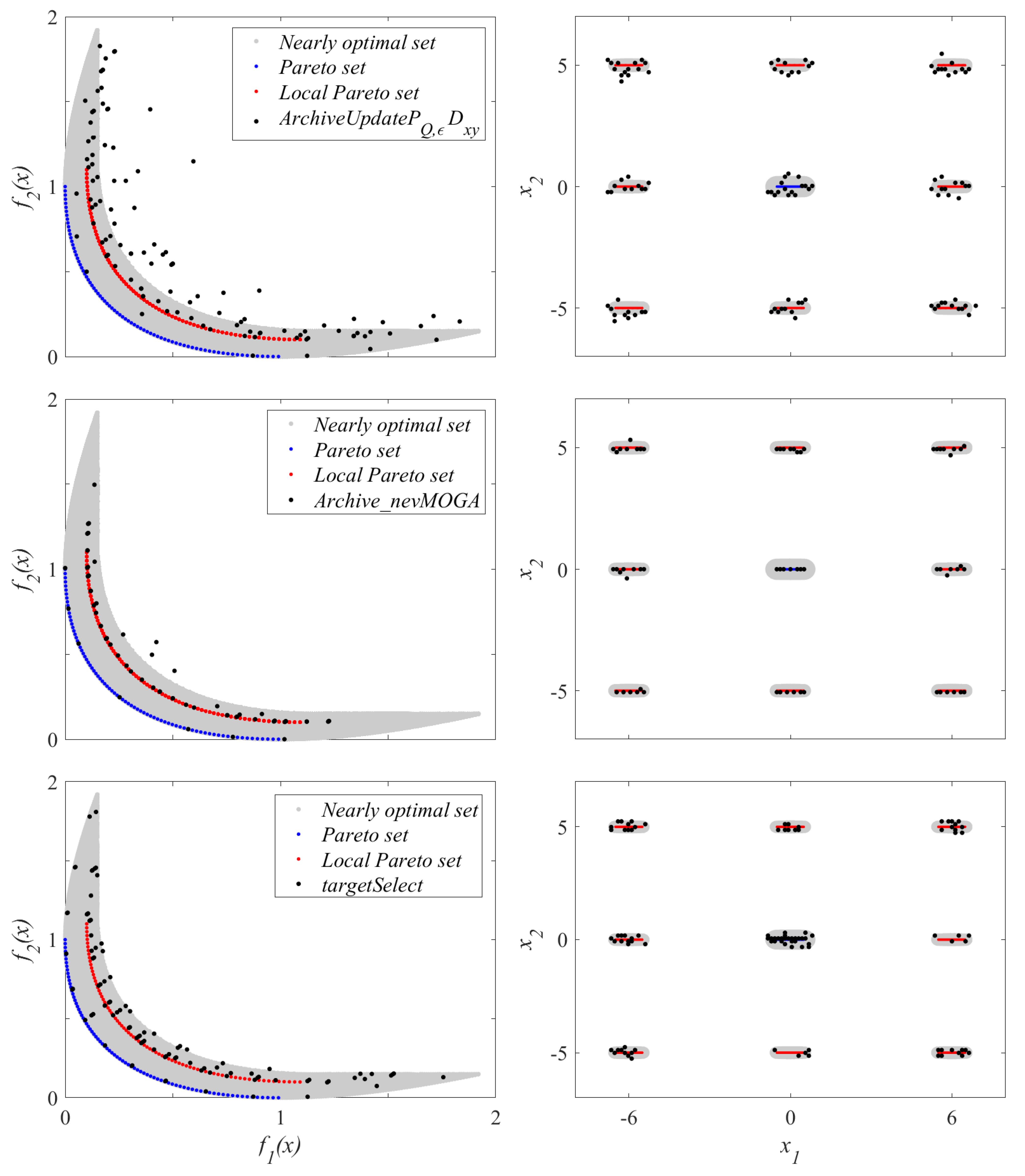
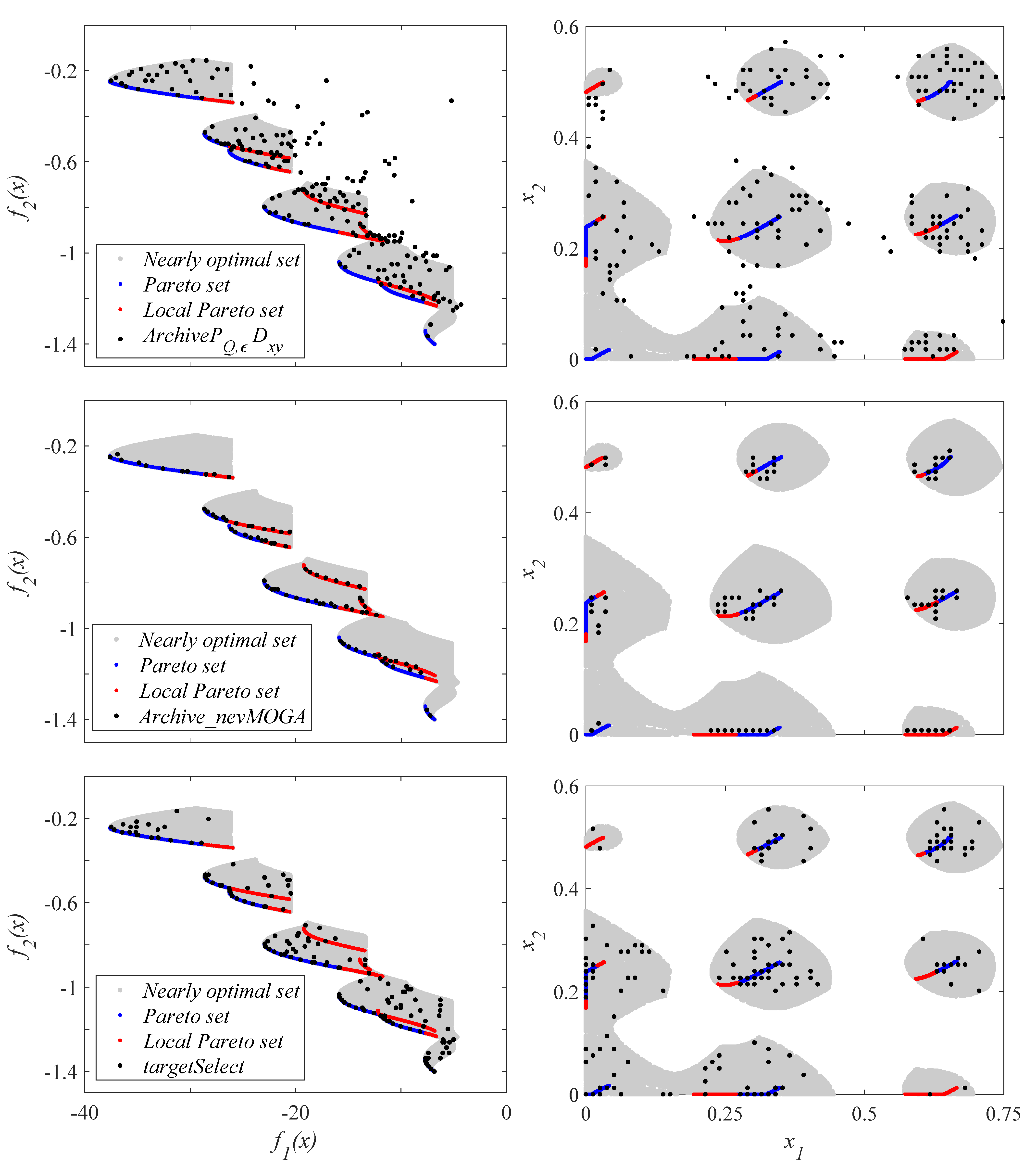
The archivers are tested on 25 different input populations obtained by uniform dispersion. Figure 7 shows the median results of archive A on the benchmark 1 for both decision and objective spaces with respect to ${\Delta }_p(A,H)$ in decision space. As can be seen, the archivers make a good approximation to the target set H, characterizing the nine neighborhoods that compose it. However, there are differences between the sets found by the archivers. First, the $Archive\_nevMOGA$ archiver obtains fewer solutions. The number of solutions ${\mu }^t=100$ for the $targetSelect$ is user-defined, but a smaller size makes ${\Delta }_p$ worse for both spaces. The archive A obtained by $ArchiveUpdate{P}_{Q,ϵ}{D}_{xy}$ obtains a larger number of solutions.

The $targetSelect$ archiver obtains a better approximation to the Pareto front than the other archivers. This is because the weight ${\omega }_o$ has a high value, giving greater weight to the $D_o$ indicator that measures convergence and diversity for the Pareto front. The $ArchiveUpdate{P}_{Q,ϵ}{D}_{xy}$ and $Archive\_nevMOGA$ archivers do not select a candidate solution p (even if p belongs to the Pareto set) if an alternative already exists in the current archive that is similar in both spaces (in $Archive\_nevMOGA$, p is selected if it dominates the similar solution). These archivers could obtain a better approximation to the Pareto front by reducing the parameter ${\Delta }_y$ (parameter with which the degree of similarity in the objective space is decided), but it probably also implies obtaining a greater number of solutions.

Regarding the local Pareto set, the archive $Archive\_nevMOGA$ obtains a better approximation in the comparison. $ArchiveUpdate{P}_{Q,ϵ}{D}_{xy}$ and $targetSelect$ obtain solutions in all neighborhoods where nearly optimal solutions exist. However, these solutions are rarely located on the lines that define the local Pareto set.

Notice that $ArchiveUpdate{P}_{Q,ϵ}{D}_{xy}$ and $Archive\_nevMOGA$ archivers obtain $ϵ-$ dominated solutions. In $ArchiveUpdate{P}_{Q,ϵ}{D}_{xy}$, it is possible that a solution in A that is no longer nearly optimal due to the apparition of a new candidate solution p. p may not be removed because it does not satisfy condition in the line 7 of Algorithm 1. In $Archive\_nevMOGA$, a new candidate solution p can be added to the archive A through the condition of line 8 of Algorithm 3. In some cases, solutions that are not nearly optimal due to the appearance of p (by line 8 of Algorithm 3) are not eliminated. Therefore, the archive A obtained by both archivers may contain solutions that do not belong to the nearly optimal set.

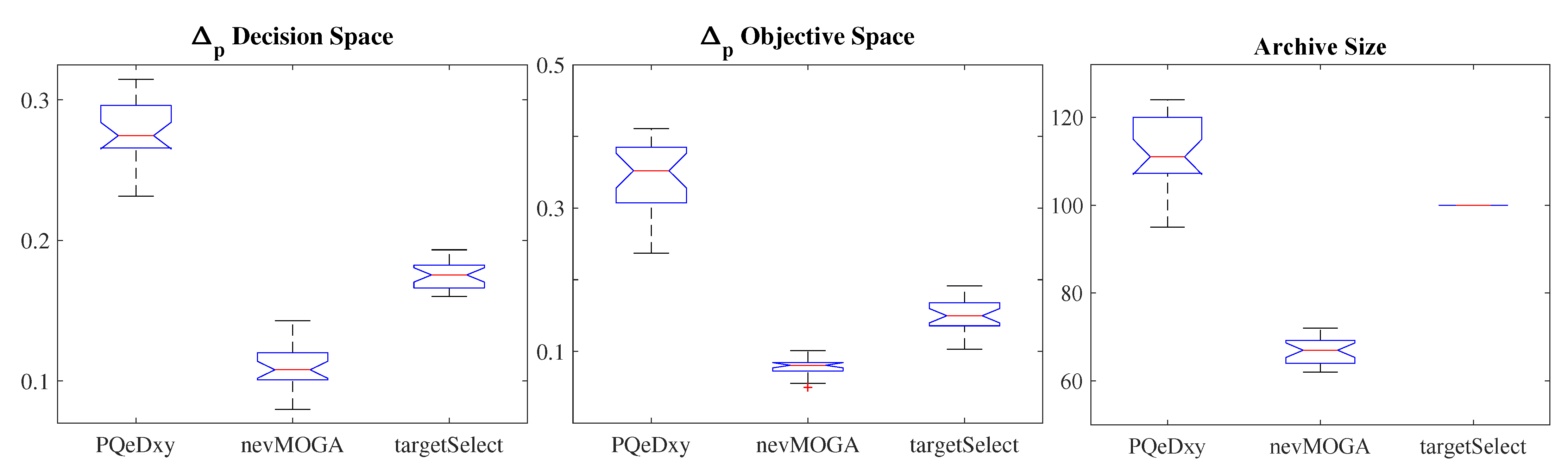
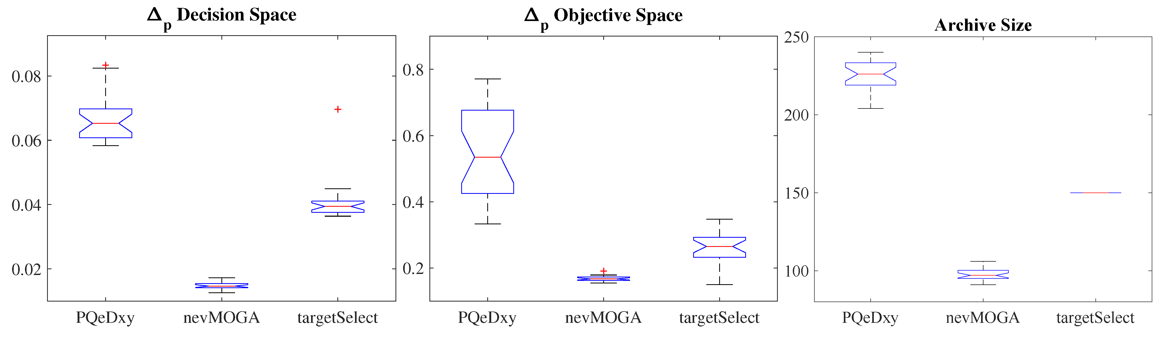
Figure 8 shows the boxplot of the indicators ${\Delta }_p(f\left(A\right),f\left(H\right))$, ${\Delta }_p(A,H)$ and archive size for the 25 tests performed. $Archive\_nevMOGA$ achieves a better approximation in the decision and objective spaces, and obtains fewer solutions. $targetSelect$ also obtains a better approximation in both spaces with fewer solutions than $ArchiveUpdate{P}_{Q,ϵ}$$D_{xy}$. $ArchiveUpdate{P}_{Q,ϵ}{D}_{xy}$ obtains greater variability among the 25 archives obtained. Therefore, $Archive\_nevMOGA$ has achieved, in a better way, the two main objectives: not neglecting the diversity of solutions (locates all nine neighborhoods) and obtains a reduced number of solutions (simplifying the optimization and decision stages).

Algorithm 3$A:=Archive\_nevMOGA(P,A_0,ϵ,{\Delta }_{\mathit{x}},{\Delta }_{\mathit{y}})$

Require: population P, archive $A_0,ϵ\in {\mathbb{R}}_{+}^m,{\Delta }_x\in {\mathbb{R}}_{+}^k,{\Delta }_y\in {\mathbb{R}}_{+}^m$

Ensure: update archive A

1: $A:=A_0$ 2: for all$p\in P$do 3:   if $(\nexists a_1\in A:a_1{\prec }_{-ϵ}p)$ and $(\nexists a_2\in A:|a_2-p|\le {\Delta }_x$ and $a_2\prec p)$ and $(\nexists a_3:|a_3-p|\le {\Delta }_x$ and $|f\left(a_3\right)-f\left(p\right)|\le {\Delta }_y)$ then 4:     $A\leftarrow A\cup p$ 5:     if $\exists a_4\in A:p{\prec }_{-ϵ}{a}_4$ or $|a_4-p|\le {\Delta }_x$ and $p\prec a_4$ then 6:       $A\leftarrow A$ \ $a_4$ 7:     end if 8:   else if $\exists a_5:|a_5-p|\le {\Delta }_x$ and $|f\left(a_5\right)-f\left(p\right)|\le {\Delta }_y$ and $p\prec a_5$ then 9:     $a_5:=p$ 10:   end if 11: end if

6.2. Benchmark 1 with Random Dispersion

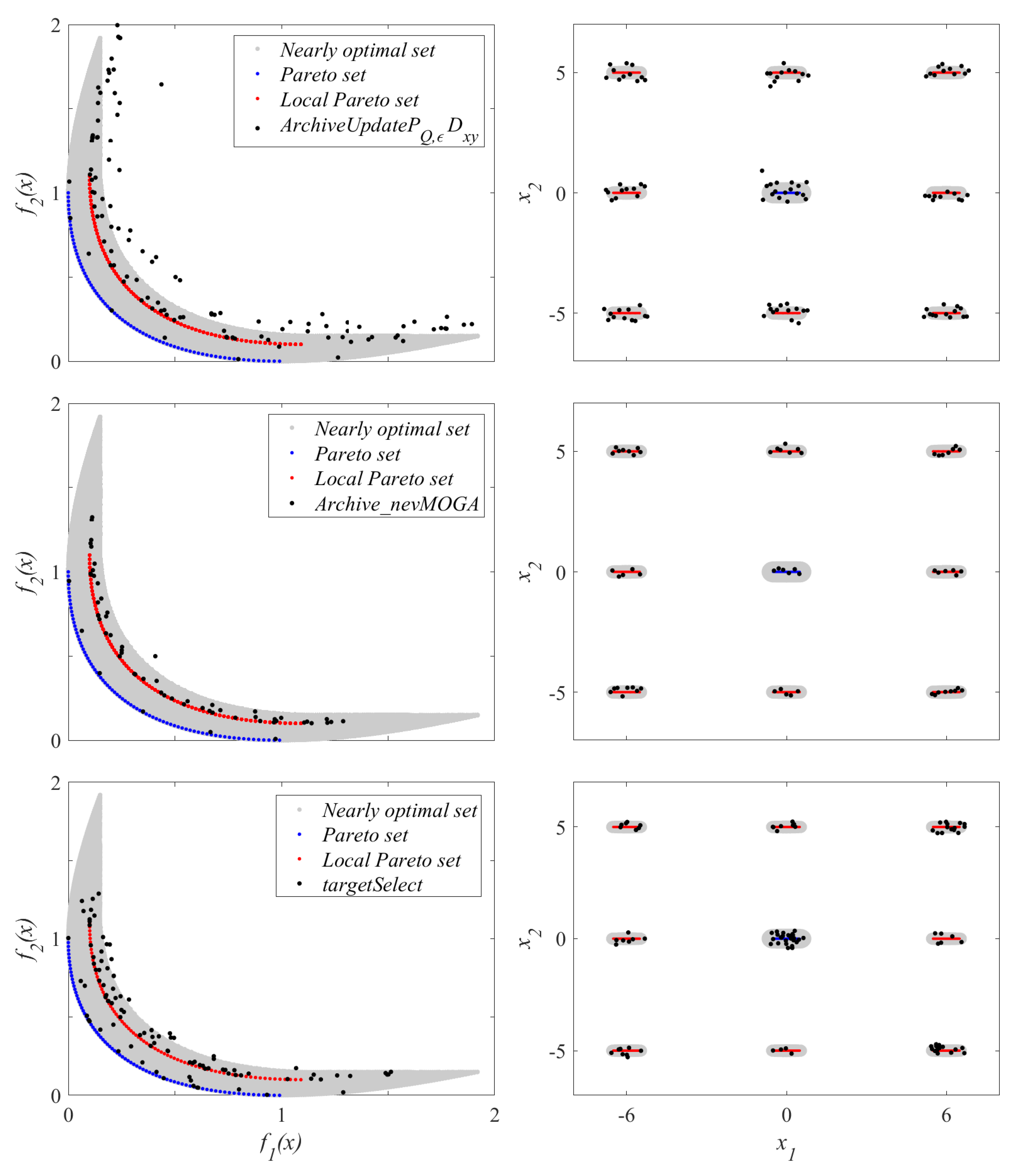
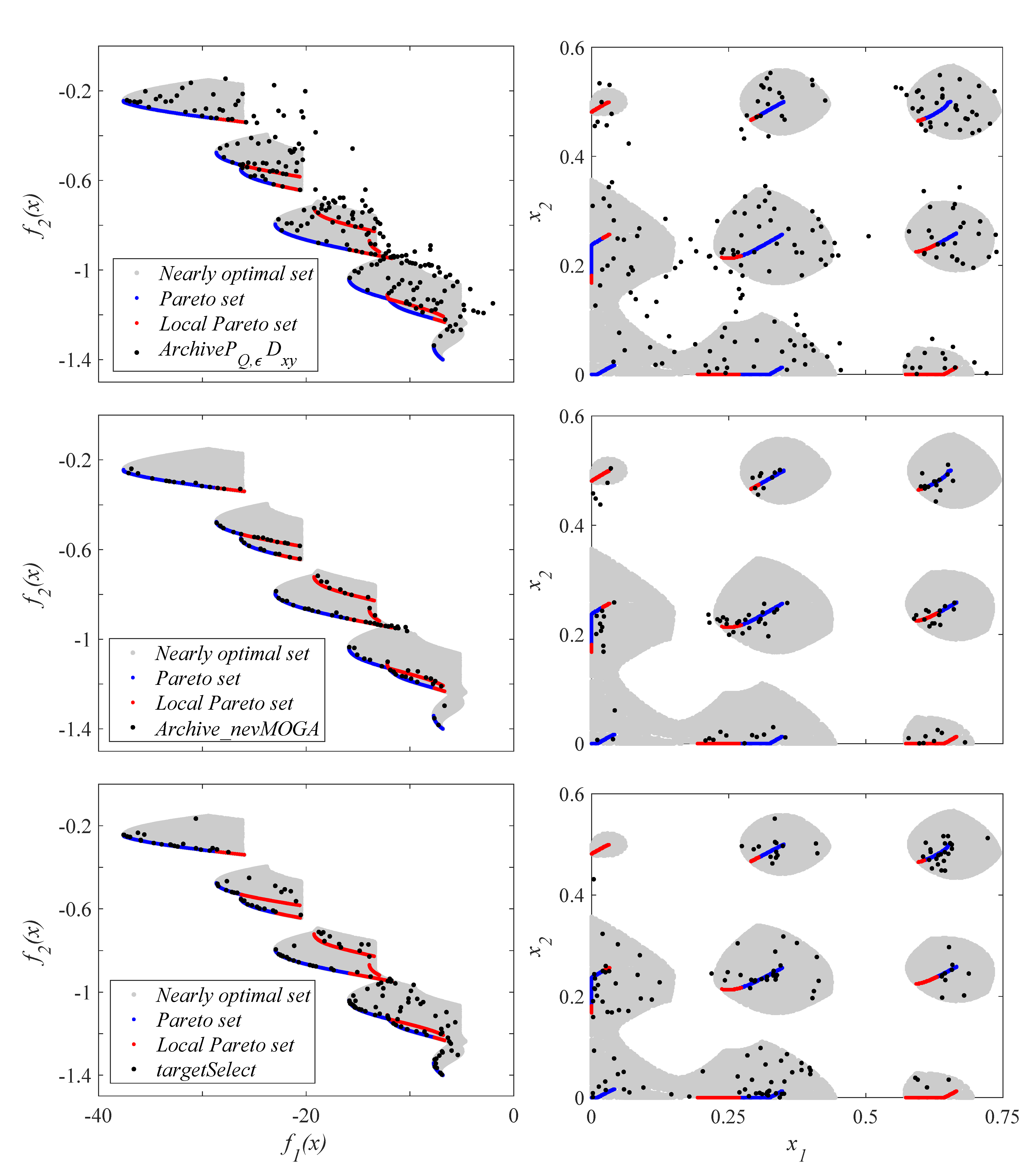
The archivers are tested on 25 different input populations obtained by random dispersion. Figure 9 shows the archive A, with median result for ${\Delta }_p(A,H)$. The archivers characterize the nine neighborhoods that form the target set H. The archive A obtained by $Archive\_nevMOGA$ has a smaller number of solutions. Decreasing the number of solutions ${\mu }^t\le 100$ for the archive $targetSelect$ makes ${\Delta }_p$ worse in both spaces. Comparing Figure 7 and Figure 9, $targetSelect$ in random dispersion produces a worse approximation of the Pareto front than in uniform search. This is for two reasons: (1) the lower value of the weight ${\omega }_o=0.7692$ (lower weight of the metric $D_o$, which measures convergence in Pareto front); (2) the initial population has been obtained in a random way (meaning certain areas have not been adequately explored). 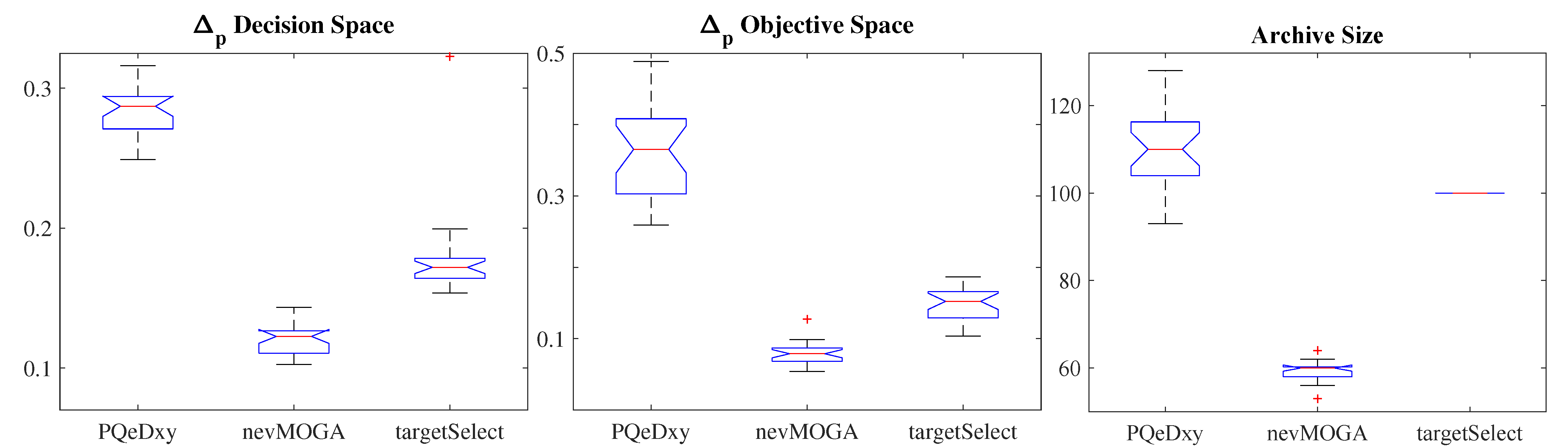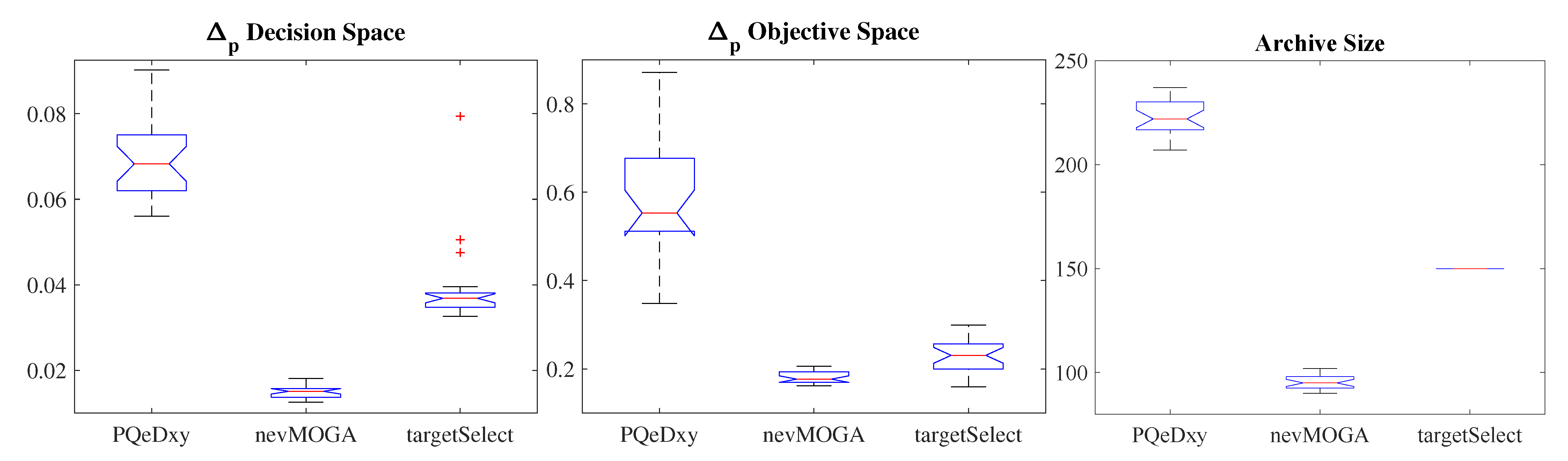Figure 10 shows the boxplot, of the 25 archives obtained in the tests. $Archive\_nevMOGA$ obtains better results in both spaces, also obtaining a smaller number of solutions. On the benchmark 1, the approximations obtained by the archivers in a random dispersion are slightly worse than in a uniform dispersion.

6.3. Benchmark 2 with Uniform Dispersion

The archive A, with the median result (in the decision space), for each archiver is shown in Figure 11. The archivers locate the neighborhoods where nearly optimal solutions are found. The archive of $Archive\_nevMOGA$ again obtains fewer solutions. Keep in mind that decreasing ${\mu }^t=150$ for $targetSelect$ causes a considerable increase in the variability of the results obtained ${\Delta }_p(A,H)$ for the 25 tests. $targetSelect$ obtains a better approximation to the Pareto front due to the high value of the weight ${\omega }_o$. However, $Archive\_nevMOGA$ obtains solutions closer to the local Pareto set. This is because $targetSelect$ seeks to achieve the greatest diversity in the decision space (through $D_d$) without taking into account whether these solutions are worse than a close solution (if they are not optimal).

Figure 12 shows the boxplot, of the 25 archives obtained for the archivers, for the indicator ${\Delta }_p$ in the decision and objective spaces and the archive size. Regarding the decision space, $Archive\_nevMOGA$ obtains a better approximation to the target set than its competitors. Regarding the objective space, $Archive\_nevMOGA$ and $targetSelect$ obtain a similar minimum value. However, $targetSelect$ obtains worse variability. Therefore, as occurred with benchmark 1, the archiver $Archive\_nevMOGA$ achieves a better approximation in both spaces and obtains a smaller number of solutions.

6.4. Benchmark 2 with Random Dispersion

Figure 13 shows the archive A, which obtains a median result for ${\Delta }_p(A,H)$ for the archivers. Again, the archiver $Archive\_nevMOGA$ obtains significantly fewer solutions while also obtaining a better characterization of the target set H. Figure 14 shows the boxplot of the archivers. The archiver $Archive\_nevMOGA$ obtains a better value of ${\Delta }_p$ in both spaces. Regarding the objective space, $targetSelect$ obtains results similar to $Archive\_nevMOGA$ but worse variability. The archiver $Archive\_nevMOGA$ obtains fewer solutions, which simplifies the optimization and decision stages. Using the random search, $ArchiveUpdate{P}_{Q,ϵ}{D}_{xy}$ and $Archive\_nevMOGA$ perform slightly worse than the uniform search. $targetSelect$ obtains slightly better results than the uniform search.

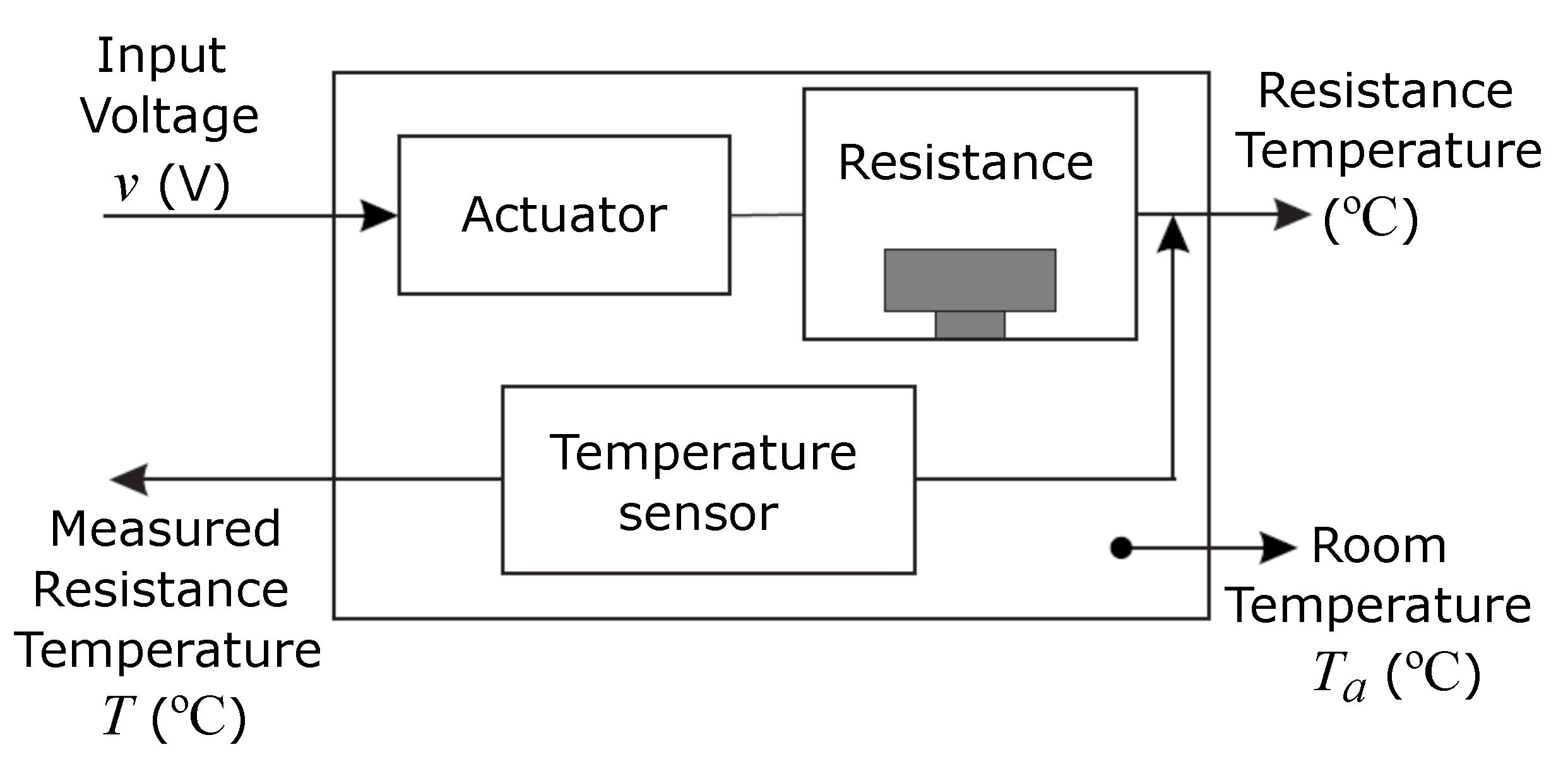
6.5. Identification of a Thermal System

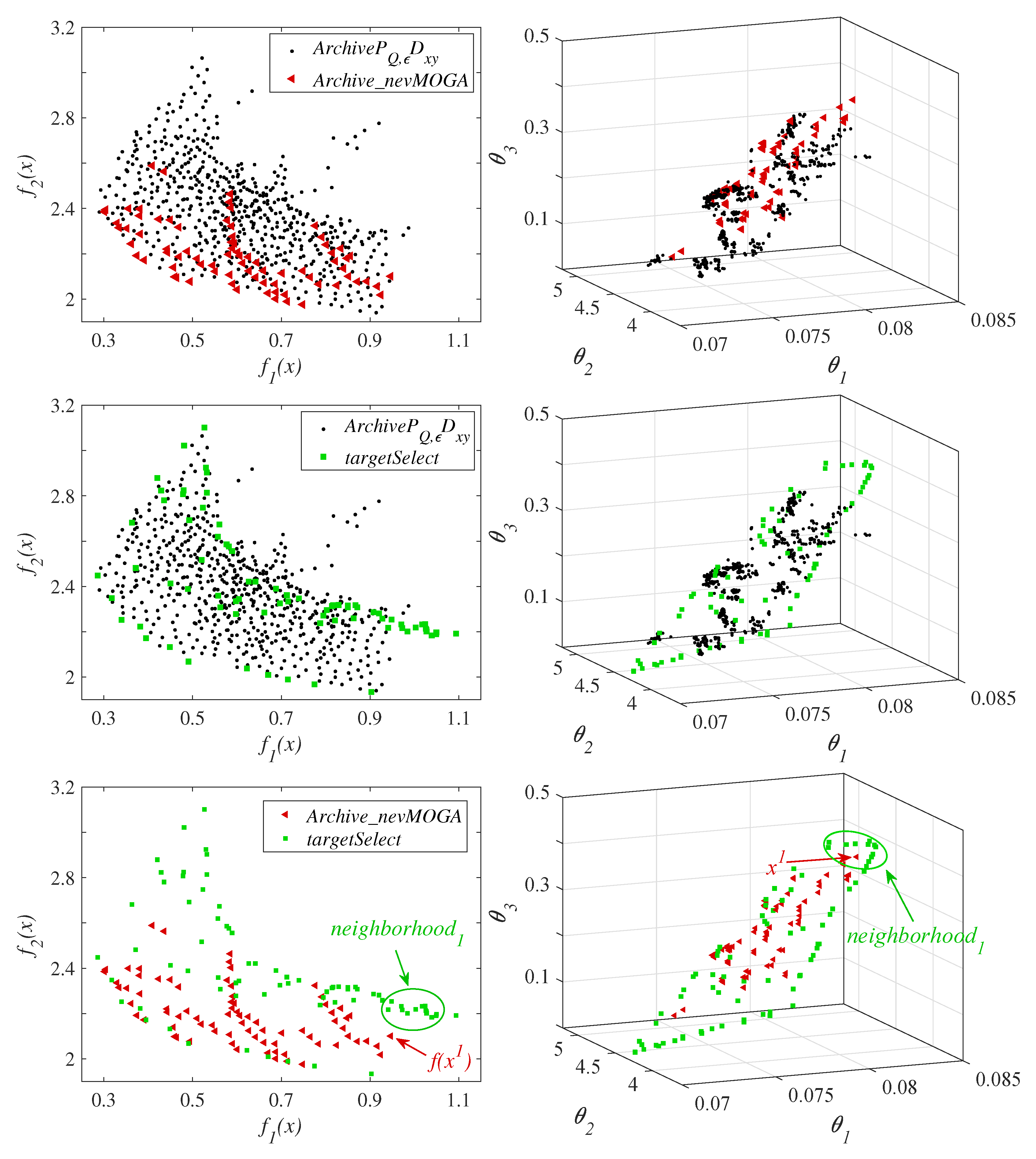
Figure 15 shows the final archive A obtained when using the three archivers inside a compared basic optimization algorithm. In this example, the obtained archives are compared by pairs to better observe the differences between them.

The three archivers obtain diversity in the decision space, and convergence in the Pareto front. The first thing that stands out is the large number of solutions (610 solutions) obtained by the archive $ArchiveUpdate{P}_{Q,ϵ}{D}_{xy}$. This high number of solutions complicates the optimization and decision phases. For each iteration, the newly generated solutions must be compared with the solutions in the current file $A\left(t\right)$. Therefore, many solutions in the file $A\left(t\right)$ implies a higher computational cost. In addition, a high number of solutions makes the final decision of the DM more difficult. This large number of solutions can be reduced by increasing the parameters ${\Delta }_x$ and ${\Delta }_y$. However, this increase also implies a worse discretization in both spaces. $ArchiveUpdate{P}_{Q,ϵ}{D}_{xy}$ obtains a worse approximation to the Pareto front.

The results show more similarities with respect to the other two archivers. Archiver $Archive\_nevMOGA$ obtains 78 solutions. To compare under similar conditions, we set the size of the file obtained by $targetSelect$ to 78 solutions (${\mu }^t=78$). In this way, both archivers obtain the same number of solutions. The set of solutions found by both archivers are different. With respect to the Pareto front, both archivers achieve a good approximation in the range $f_1\left(x\right)=[0.3 0.8]$. However, $Archive\_nevMOGA$ does not get solutions in the range $f_1\left(x\right)=[0.8 0.9]$ of the Pareto front. Therefore, in this example, $targetselect$ gets a little more diversity in the Pareto front.

$targetSelect$ focuses on obtaining, in addition to a good convergence in the Pareto front, the greatest diversity in the decision space (using $D_d$, see Section 4.3). However, solutions that provide greater diversity may be worse than neighboring solutions. For example, Figure 15 shows the solution ${\mathit{x}}^{\mathbf{1}}$ obtained by $Archive\_nevMOGA$. This solution has similar parameters to the $neighborhoo{d}_1$ solutions (see decision space). ${\mathit{x}}^{\mathbf{1}}$ performs better ($\mathit{f}\left({\mathit{x}}^{\mathbf{1}}\right)$) than all the $neighborhoo{d}_1$ solutions obtained by $targetSelect$. Therefore, $Archive\_nevMOGA$ would eliminate all these solutions (dominated in its neighborhood by ${\mathit{x}}^{\mathbf{1}}$). $targetSelect$ maintains them because they increase the diversity in the decision space. This happens repeatedly in this MOOP. For this reason, $targetSelect$ obtains nearly optimal solutions farther from the Pareto front than obtained by $Archive\_nevMOGA$. These solutions are in the contour/ends of the plane that form the optimal and nearly optimal solutions in the decision space, and therefore, they obtain a better diversity under the $D_d$ indicator. $Archive\_nevMOGA$ could find solutions closer to the contour/ends of the plane formed in the decision space (as is the case with $targetSelect$) by reducing the parameter ${\Delta }_{\mathit{x}}$, although this would imply obtaining a larger number of solutions. Therefore, depending on the needs or preferences of the DM, the use of one archiver or another may be more appropriate. This archiver can be embedded in most of the multi-objective algorithms available. $ArchiveUpdate{P}_{Q,ϵ}{D}_{xy}$, $Archive\_nevMOGA$ and $targetSelect$ archivers are currently built into the algorithms N$ϵ$SGA, $nevMOGA$ and $DIOP$ respectively.

7. Conclusions

In this paper, the characterization of nearly optimal solutions potentially useful in a MOOP has been addressed. In this type of problem, in practice, the DM may wish to obtain nearly optimal solutions, since they can play a relevant role in the decision-making stage. However, an adequate approximation to this set is necessary to avoid an excessive number of alternatives that could hinder the optimization and decision-making stages. Not all nearly optimal solutions provide the same useful information to the DM. To reduce the number of solutions to be analyzed, we consider potentially useful solutions (in addition to the optimals) that are close to the optimals in objective space—but which differ significantly in the decision space. To adequately characterize this set, it is necessary to discretize the nearly optimal solutions by analyzing the decision and objective spaces simultaneously.

This article compares different archiving strategies that perform this task: $Archive$- $Update{P}_{Q,ϵ}{D}_{xy}$, $Archive\_nevMOGA$ and $targetSelect$. The main objective of the archivers is to obtain potentially useful solutions. This analysis is of great help to designers of evolutionary algorithms who wish to obtain such solutions. In this way, designers will have more information to choose their archivers based on their preferences. $ArchiveUpdate{P}_{Q,ϵ}{D}_{xy}$ and $Archive\_nevMOGA$ are two distance-based archivers. Both archivers simultaneously discard solutions that are similar in decision and objective spaces. However, $Archive\_nevMOGA$, in contrast to $ArchiveUpdate{P}_{Q,ϵ}{D}_{xy}$, discards solutions dominated by a neighboring solution in the decision space. $targetSelect$ is an archive based on an indicator that measures the diversity in both spaces simultaneously. $targetSelect$, unlike the other archivers, can directly and arbitrarily specify the archive size. This can be an advantage. The archivers are evaluated using two benchmarks. They obtain a good approximation to the set of potentially useful solutions, characterizing the diversity existing in the set of nearly optimal solutions. As discussed in [19], the $ArchiveUpdate{P}_{Q,ϵ}{D}_{xy}$ archiver is more practical than other archivers in the literature. However, this archiver, as demonstrated in this paper, obtains significantly more solutions than its competitors in this paper. This can make the optimization and decision phase more difficult. In addition, $Archive\_nevMOGA$ obtains a better approximation to the target set H under the averaged Hausdorff distance ${\Delta }_p$. In addition, $Archive\_nevMOGA$ obtains a smaller number of solutions, which speeds up the optimization process and facilitates the decision-making stage. However, fewer solutions can also decrease diversity (which can lead to degraded global search capabilities).

Finally, the compared archivers are analyzed on a real engineering example. This real example is the identification of a thermal system. To carry out this analysis, a generic multi-objective optimization algorithm is used, in which it is possible to select different archivers. This enables a more realistic comparison of the impact of the archivers on the entire optimization process.

The three archivers obtain the existing diversity in the set of optimal and nearly optimal solutions. In this last example, we can see how the archive obtained by $ArchiveUpdate{P}_{Q,ϵ}{D}_{xy}$ obtains a very high number of solutions, complicating the optimization and decision stages. $Archive\_nevMOGA$ and $targetSelect$ obtain the same number of solutions. Both archivers obtain an adequate Pareto front. However, $targetSelect$ gets more diversity on the Pareto front. The main difference between the two archivers is in the set of nearly optimal solutions. On the one hand, $Archive\_nevMOGA$ obtains solutions closer to the Pareto front, but significantly different in the decision space. On the other hand, $targetSelect$ obtains the solutions that provide the greatest diversity in the decision space, even though these solutions are farther away from the Pareto front, and therefore, offer significantly worse performance.

Finally, this analysis suggests two possible future lines of research: (1) design of new evolutionary algorithms, which characterize the nearly optimal solutions, using some of the archivers compared in this work and (2) design of new archivers that improve the current ones. For example, the clustering techniques could improve the archivers compared in this work. These techniques, not analyzed in this work, allow the location of new neighborhoods, allowing their exploration and evaluation. In this way, the optimization process could be improved.

References

1. Rhinehart, R.R. Engineering Optimization: Applications, Methods and Analysis; John Wiley & Sons: Hoboken, NJ, USA, 2018. [Google Scholar]
2. Rao, S.S. Engineering Optimization: Theory and Practice; John Wiley & Sons: Hoboken, NJ, USA, 2019. [Google Scholar]
3. Dai, C.; Lei, X. A multiobjective brain storm optimization algorithm based on decomposition. Complexity 2019, 2019. [Google Scholar] [CrossRef]
4. Miettinen, K. Nonlinear Multiobjective Optimization; Springer Science & Business Media: Berlin/Heidelberg, Germany, 2012; Volume 12. [Google Scholar]
5. Deb, K. Multi-Objective Optimization Using Evolutionary Algorithms; John Wiley & Sons: Hoboken, NJ, USA, 2001; Volume 16. [Google Scholar]
6. Reynoso-Meza, G.; Blasco, X.; Sanchis, J.; Herrero, J.M. Controller Tuning with Evolutionary Multiobjective Optimization: A Holistic Multiobjective Optimization Design Procedure; Springer: Berlin/Heidelberg, Germany, 2017. [Google Scholar]
7. Gunantara, N. A review of multi-objective optimization: Methods and its applications. Cogent Eng. 2018, 5, 1502242. [Google Scholar] [CrossRef]
8. Sanchis, J.; Martínez, M.A.; Blasco, X. Integrated multiobjective optimization and a priori preferences using genetic algorithms. Inf. Sci. 2008, 178, 931–951. [Google Scholar] [CrossRef]
9. Zitzler, E.; Deb, K.; Thiele, L. Comparison of multiobjective evolutionary algorithms: Empirical results. Evol. Comput. 2000, 8, 173–195. [Google Scholar] [CrossRef] [Green Version]
10. Ulrich, T.; Bader, J.; Thiele, L. Defining and optimizing indicator-based diversity measures in multiobjective search. In International Conference on Parallel Problem Solving from Nature; Springer: Berlin/Heidelberg, Germany, 2010; pp. 707–717. [Google Scholar]
11. Beyer, H.G.; Sendhoff, B. Robust optimization—A comprehensive survey. Comput. Methods Appl. Mech. Eng. 2007, 196, 3190–3218. [Google Scholar] [CrossRef]
12. Jin, Y.; Branke, J. Evolutionary optimization in uncertain environments—A survey. IEEE Trans. Evol. Comput. 2005, 9, 303–317. [Google Scholar] [CrossRef] [Green Version]
13. Deb, K.; Gupta, H. Introducing robustness in multi-objective optimization. Evol. Comput. 2006, 14, 463–494. [Google Scholar] [CrossRef]
14. Pajares, A.; Blasco, X.; Herrero, J.M.; Reynoso-Meza, G. A new point of view in multivariable controller tuning under multiobjetive optimization by considering nearly optimal solutions. IEEE Access 2019, 7, 66435–66452. [Google Scholar] [CrossRef]
15. Loridan, P. ε-solutions in vector minimization problems. J. Optim. Theory Appl. 1984, 43, 265–276. [Google Scholar] [CrossRef]
16. White, D.J. Epsilon efficiency. J. Optim. Theory Appl. 1986, 49, 319–337. [Google Scholar] [CrossRef]
17. Engau, A.; Wiecek, M.M. Generating ε-efficient solutions in multiobjective programming. Eur. J. Oper. Res. 2007, 177, 1566–1579. [Google Scholar] [CrossRef]
18. Hernández Castellanos, C.I.; Schütze, O.; Sun, J.Q.; Ober-Blöbaum, S. Non-Epsilon Dominated Evolutionary Algorithm for the Set of Approximate Solutions. Math. Comput. Appl. 2020, 25, 3. [Google Scholar] [CrossRef] [Green Version]
19. Schütze, O.; Hernandez, C.; Talbi, E.G.; Sun, J.Q.; Naranjani, Y.; Xiong, F.R. Archivers for the representation of the set of approximate solutions for MOPs. J. Heuristics 2019, 25, 71–105. [Google Scholar] [CrossRef]
20. Tanabe, R.; Ishibuchi, H. A review of evolutionary multimodal multiobjective optimization. IEEE Trans. Evol. Comput. 2019, 24, 193–200. [Google Scholar] [CrossRef]
21. Li, M.; Yao, X. An empirical investigation of the optimality and monotonicity properties of multiobjective archiving methods. In International Conference on Evolutionary Multi-Criterion Optimization; Springer: Berlin/Heidelberg, Germany, 2019; pp. 15–26. [Google Scholar]
22. Knowles, J.D.; Corne, D.W. Approximating the nondominated front using the Pareto archived evolution strategy. Evol. Comput. 2000, 8, 149–172. [Google Scholar] [CrossRef] [PubMed]
23. Laumanns, M.; Thiele, L.; Deb, K.; Zitzler, E. Combining convergence and diversity in evolutionary multiobjective optimization. Evol. Comput. 2002, 10, 263–282. [Google Scholar] [CrossRef]
24. Schütze, O.; Laumanns, M.; Coello, C.A.C.; Dellnitz, M.; Talbi, E.G. Convergence of stochastic search algorithms to finite size Pareto set approximations. J. Glob. Optim. 2008, 41, 559–577. [Google Scholar] [CrossRef] [Green Version]
25. Schütze, O.; Lara, A.; Coello, C.A.C.; Vasile, M. Computing approximate solutions of scalar optimization problems and applications in space mission design. In Proceedings of the IEEE Congress on Evolutionary Computation, Barcelona, Spain, 18–23 July 2010; pp. 1–8. [Google Scholar]
26. Zhou, X.; Long, J.; Xu, C.; Jia, G. An external archive-based constrained state transition algorithm for optimal power dispatch. Complexity 2019, 2019. [Google Scholar] [CrossRef]
27. Schütze, O.; Hernández, C. Archiving Strategies for Evolutionary Multi-Objective Optimization Algorithms; Springer: Berlin/Heidelberg, Germany, 2021. [Google Scholar]
28. Schütze, O.; Vasile, M.; Coello, C.A.C. Approximate solutions in space mission design. In International Conference on Parallel Problem Solving from Nature; Springer: Berlin/Heidelberg, Germany, 2008; pp. 805–814. [Google Scholar]
29. Pajares, A.; Blasco, X.; Herrero, J.M.; Reynoso-Meza, G. A multiobjective genetic algorithm for the localization of optimal and nearly optimal solutions which are potentially useful: nevMOGA. Complexity 2018, 2018. [Google Scholar] [CrossRef]
30. Schütze, O.; Vasile, M.; Coello, C.A.C. Computing the set of epsilon-efficient solutions in multiobjective space mission design. J. Aerosp. Comput. Inf. Commun. 2011, 8, 53–70. [Google Scholar] [CrossRef] [Green Version]
31. Pareto, V. Manual of Political Economy; Oxford University Press: Oxford, UK, 1971. [Google Scholar]
32. Schütze, O.; Coello, C.A.C.; Talbi, E.G. Approximating the ε-efficient set of an MOP with stochastic search algorithms. In Mexican International Conference on Artificial Intelligence; Springer: Berlin/Heidelberg, Germany, 2007; pp. 128–138. [Google Scholar]
33. Teytaud, O. On the hardness of offline multi-objective optimization. Evol. Comput. 2007, 15, 475–491. [Google Scholar] [CrossRef] [PubMed]
34. Schütze, O.; Esquivel, X.; Lara, A.; Coello, C.A.C. Using the averaged Hausdorff distance as a performance measure in evolutionary multiobjective optimization. IEEE Trans. Evol. Comput. 2012, 16, 504–522. [Google Scholar] [CrossRef]
35. Karimi, D.; Salcudean, S.E. Reducing the hausdorff distance in medical image segmentation with convolutional neural networks. IEEE Trans. Med. Imaging 2019, 39, 499–513. [Google Scholar] [CrossRef] [Green Version]
36. Van Veldhuizen, D.A.; Lamont, G.B. Multiobjective Evolutionary Algorithm Research: A History and Analysis; Technical Report; Air Force Institute of Technology: Dayton, OH, USA, 1998. [Google Scholar]
37. Zhou, A.; Jin, Y.; Zhang, Q.; Sendhoff, B.; Tsang, E. Combining model-based and genetics-based offspring generation for multi-objective optimization using a convergence criterion. In Proceedings of the 2006 IEEE International Conference on Evolutionary Computation, Vancouver, BC, Canada, 16–21 July 2006; pp. 892–899. [Google Scholar]
38. Mahbub, M.S.; Wagner, T.; Crema, L. Improving robustness of stopping multi-objective evolutionary algorithms by simultaneously monitoring objective and decision space. In Proceedings of the 2015 Annual Conference on Genetic and Evolutionary Computation, Lille, France, 10–14 July 2015; pp. 711–718. [Google Scholar]
39. Khare, V.; Yao, X.; Deb, K. Performance scaling of multi-objective evolutionary algorithms. In International Conference on Evolutionary Multi-Criterion Optimization; Springer: Berlin/Heidelberg, Germany, 2003; pp. 376–390. [Google Scholar]
40. Sebag, M.; Tarrisson, N.; Teytaud, O.; Lefevre, J.; Baillet, S. A Multi-Objective Multi-Modal Optimization Approach for Mining Stable Spatio-Temporal Patterns. In Proceedings of the 19th International Joint Conference on Artificial Intelligence, Edinburgh, UK, 30 July–5 August 2005; pp. 859–864. [Google Scholar]
41. Krmicek, V.; Sebag, M. Functional brain imaging with multi-objective multi-modal evolutionary optimization. In Parallel Problem Solving from Nature-PPSN IX; Springer: Berlin/Heidelberg, Germany, 2006; pp. 382–391. [Google Scholar]
42. Zechman, E.M.; Giacomoni, M.H.; Shafiee, M.E. An evolutionary algorithm approach to generate distinct sets of non-dominated solutions for wicked problems. Eng. Appl. Artif. Intell. 2013, 26, 1442–1457. [Google Scholar] [CrossRef]
43. Deb, K.; Agrawal, S.; Pratap, A.; Meyarivan, T. A fast elitist non-dominated sorting genetic algorithm for multi-objective optimization: NSGA-II. In International Conference on Parallel Problem Solving from Nature; Springer: Berlin/Heidelberg, Germany, 2000; pp. 849–858. [Google Scholar]
44. Hernández Castellanos, C.I. Set Oriented Methods for Multi-Objective Optimization. Ph.D. Thesis, Centro de Investigación y de Estudios Avanzados del Instituto Politécnico Nacional, Mexico City, Mexico, 2017. [Google Scholar]
45. Ulrich, T.; Bader, J.; Zitzler, E. Integrating decision space diversity into hypervolume-based multiobjective search. In Proceedings of the 12th Annual Conference on Genetic and Evolutionary Computation, Portland, OR, USA, 7–11 July 2010; pp. 455–462. [Google Scholar]
46. Solow, A.R.; Polasky, S. Measuring biological diversity. Environ. Ecol. Stat. 1994, 1, 95–103. [Google Scholar] [CrossRef]
47. Rudolph, G.; Naujoks, B.; Preuss, M. Capabilities of EMOA to detect and preserve equivalent Pareto subsets. In International Conference on Evolutionary Multi-Criterion Optimization; Springer: Berlin/Heidelberg, Germany, 2007; pp. 36–50. [Google Scholar]
48. Zhang, K.; Chen, M.; Xu, X.; Yen, G.G. Multi-objective evolution strategy for multimodal multi-objective optimization. Appl. Soft Comput. 2021, 101, 107004. [Google Scholar] [CrossRef]
49. Yue, C.; Qu, B.; Liang, J. A multiobjective particle swarm optimizer using ring topology for solving multimodal multiobjective problems. IEEE Trans. Evol. Comput. 2017, 22, 805–817. [Google Scholar] [CrossRef]
50. Zhang, X.; Liu, H.; Tu, L. A modified particle swarm optimization for multimodal multi-objective optimization. Eng. Appl. Artif. Intell. 2020, 95, 103905. [Google Scholar] [CrossRef]
51. Li, X.; Engelbrecht, A.; Epitropakis, M.G. Benchmark Functions for CEC’2013 Special Session and Competition on Niching Methods for Multimodal Function Optimization; RMIT University, Evolutionary Computation and Machine Learning Group: Melbourne, Australia, 2013. [Google Scholar]
52. Wang, H.; Jin, Y.; Doherty, J. Committee-based active learning for surrogate-assisted particle swarm optimization of expensive problems. IEEE Trans. Cybern. 2017, 47, 2664–2677. [Google Scholar] [CrossRef] [Green Version]
53. Ariyaratne, M.; Fernando, T.; Weerakoon, S. A Hybrid Algorithm to Solve Multi-model Optimization Problems Based on the Particle Swarm Optimization with a Modified Firefly Algorithm. In Proceedings of the Future Technologies Conference; Springer: Berlin/Heidelberg, Germany, 2020; pp. 308–325. [Google Scholar]
54. Marek, M.; Kadlec, P.; Čapek, M. FOPS: A new framework for the optimization with variable number of dimensions. Int. J. RF Microw. Comput. Aided Eng. 2020, 30, e22335. [Google Scholar] [CrossRef]
55. Lienhard, I.; John, H. A Heat Transfer Textbook; Phlogiston Press: Cambridge, MA, USA, 2005. [Google Scholar]
56. Deb, K.; Agrawal, R.B. Simulated binary crossover for continuous search space. Complex Syst. 1995, 9, 115–148. [Google Scholar]
Figure 1. A MOOP example. On the left, the objective space is shown, and on the right, the decision space is shown. S E T 1 is the Pareto optimal set and S E T 2 is a potentially useful nearly optimal set.
Mathematics 09 00999 g001
Figure 2. Visualization of an MOOP in the objective space (on the left) and decision space (on the right). The sets S E T 1 and S E T 2 are the optimal solutions. Both sets and S E T 3 and S E T 4 form the local Pareto set.
Mathematics 09 00999 g002
Figure 3. Target set H for the benchmark 1 formed by the global (blue) and local (red) Pareto set.
Mathematics 09 00999 g003
Figure 4. Target set H for the benchmark 2 formed by the global (blue) and local (red) Pareto set.
Mathematics 09 00999 g004
Figure 5. Block diagram of the thermal system.
Mathematics 09 00999 g005
Figure 6. Identification test of the thermal system.
Mathematics 09 00999 g006
Figure 7. Median result of archive A obtained by A r c h i v e U p d a t e P Q , ϵ D x y , A r c h i v e _ n e v M O G A and t a r g e t S e l e c t with a uniform dispersion on benchmark 1.
Mathematics 09 00999 g007
Figure 8. Boxplot of Δ p ( A , H ) (decision space), Δ p ( f ( A ) , f ( H ) ) (objective space) and archive size with a uniform dispersion on the benchmark 1.
Mathematics 09 00999 g008
Figure 9. Median result of Archive A obtained by A r c h i v e U p d a t e P Q , ϵ D x y , A r c h i v e _ n e v M O G A and t a r g e t S e l e c t with a random dispersion on benchmark 1.
Mathematics 09 00999 g009
Figure 10. Boxplot of Δ p ( A , H ) (decision space), Δ p ( f ( A ) , f ( H ) ) (objective space) and archive size with a random dispersion on the benchmark 1.
Mathematics 09 00999 g010
Figure 11. Median result of archive A obtained by A r c h i v e U p d a t e P Q , ϵ D x y , A r c h i v e _ n e v M O G A and t a r g e t S e l e c t with a uniform dispersion on the benchmark 2.
Mathematics 09 00999 g011
Figure 12. Boxplot of Δ p ( A , H ) (decision space), Δ p ( f ( A ) , f ( H ) ) (objective space) and archive size with a uniform dispersion on the benchmark 2.
Mathematics 09 00999 g012
Figure 13. Median result of Archive A obtained by A r c h i v e U p d a t e P Q , ϵ D x y , A r c h i v e _ n e v M O G A and t a r g e t S e l e c t with a random dispersion on benchmark 2.
Mathematics 09 00999 g013
Figure 14. Boxplot of Δ p ( A , H ) (decision space), Δ p ( f ( A ) , f ( H ) ) (objective space) and archive size with a random dispersion on the benchmark 2.
Mathematics 09 00999 g014
Figure 15. Archive A obtained with a generic algorithm and the archivers A r c h i v e U p d a t e P Q , ϵ D x y , A r c h i v e _ n e v M O G A and t a r g e t S e l e c t for the identification of the thermal system.
Mathematics 09 00999 g015