EM Estimation for the Bivariate Mixed Exponential Regression Model

Abstract

In this paper, we present a new family of bivariate mixed exponential regression models for taking into account the positive correlation between the cost of claims from motor third party liability bodily injury and property damage in a versatile manner. Furthermore, we demonstrate how maximum likelihood estimation of the model parameters can be achieved via a novel Expectation-Maximization algorithm. The implementation of two members of this family, namely the bivariate Pareto or, Exponential-Inverse Gamma, and bivariate Exponential-Inverse Gaussian regression models is illustrated by a real data application which involves fitting motor insurance data from a European motor insurance company.

1. Introduction

Over the last few decades, there has been a vast increase in actuarial research works focusing on modeling costs of a particular claim type based on various claim severity modeling approaches such as

• finite mixture models: see, for example, (Fung et al. 2021; Lee and Lin 2010; Miljkovic and Grün 2016; Tzougas et al. 2014, 2018, 2019);
• composite or splicing models: see for instance, (Bakar et al. 2015; Calderín-Ojeda and Kwok 2016; Cooray and Ananda 2005; Grün and Miljkovic 2019; Nadarajah and Bakar 2014; Parodi 2020; Pigeon and Denuit 2011; Scollnik 2007; Scollnik and Sun 2012).
• combinations of finite mixtures and composite models: see Reynkens et al. (2017).

Furthermore, several works have focused on understanding how the claim severity distribution is influenced by certain risk factors. See, for example, (Frees 2009; Laudagé et al. 2019; Tzougas and Jeong 2021; Tzougas and Karlis 2020) among many more. However, even if the literature in the univariate setting is abundant, the bivariate, and/or multivariate, extensions of such models have not been explored in depth even if in non-life insurance, the actuary may often be concerned with modeling jointly different types of claims and their associated costs.

In this paper, motivated by a European Motor Third Party Liability (MTPL) insurance data set which is described in Section 4 we introduce a family of bivariate mixed Exponential regression models for joint modeling the costs from positively correlated bodily injury and property damage claims in terms of covariates. The proposed class of bivariate claim severity regression models is based on a mixing between two marginal Exponential distributions and a unit mean continuous and at least twice differentiable mixing density. The modeling framework we consider can account for the positive dependency between the two claim types in a flexible manner since it allows for a variety of alternative distributional assumptions for the mixing density. Furthermore, depending on the choice of the mixing density the bivariate mixed Exponential model can be used to model both moderate and large bodily injury and property damage claim sizes which can be the result of the same accident. At this point, it is worth noting that modeling positively correlated claims and their associated counts for the same and/or different types of coverage, such as home and auto insurance, bundled together under a single policy, has been explored by many articles. See for example, (Bermúdez and Karlis 2011, 2012, 2017, 2021; Shi and Valdez 2014a, 2014b; Abdallah et al. 2016; Bermúdez et al. 2018; Pechon et al. 2018, 2019, 2021; Bolancé and Vernic 2019; Denuit et al. 2019; Fung et al. 2019; Bolancé et al. 2020; Jeong and Dey 2021; Gómez-Déniz and Calderín-Ojeda 2021; Tzougas and di Cerchiara 2021a, 2021b). Furthermore, Baumgartner et al. (2015) and Oh et al. (2021) consider shared random effects for capturing possible associations between the frequency and severity and/or among the longitudinal claims. However, with the exception of the bivariate, and/or multivariate Pareto model which have been actively studied in the actuarial literature for the case with and without covariates, see, for instance, Yang et al. (2011), Cockriel and McDonald (2018) and Jeong and Valdez (2020), modeling positively correlated claim sizes based on alternative e bivariate, and/or multivariate, mixed Exponential regression models remains a largely uncharted research territory. Therefore, this is the main contribution of this study from a practical insurance business perspective. Additionally, our contribution from a computational maximum likelihood (ML) estimation standpoint is that we develop an Expectation-Maximization (EM) type algorithm1 which takes advantage of the stochastic mixture representation of the bivariate mixed Exponential regression model for maximizing its log-likelihood in a computationally efficient and parsimonious manner. For expository purposes, the bivariate Pareto (BPA), or Exponential-Inverse Gamma, and bivariate Exponential-Inverse Gaussian (BEIG) regression models are fitted on the MTPL bodily injury and property damage data set.

Finally, it should be noted that when dealing with different types of claims from different types of coverage, such as motor and home insurance, the regressors on the mean parameters may differ according to different individual and coverage-type risk factors. However, in the case of our MTPL data, both mean parameters of the bivariate mixed Exponential regression model are only modeled using common explanatory variables for both claim types. Thus, we extend the proposed setup by pairing a bivariate Normal copula with the PA and EIG regression models. These copula-based models, which can cope with both positive and negative dependence structures, are compared with the BPA and BEIG regression models using a simulated data set in which we assume that we have different types of claims from different types of cover.

The rest of the paper proceeds as follows. Section 2 discusses how the bivariate mixed exponential regression model can be constructed and the joint probability density functions (jpdfs) of the BPA and BEIG regression models, which are used for demonstration purposes, are derived. Section 3 deals with parameter estimation for the proposed model based on the EM algorithm. In Section 4, the models presented in Section 2 are fitted to the MTPL bodily injury and property damage claims data set and the comparison based on the simulated data set mentioned in the previous paragraph is presented. Finally, concluding remarks are provided in Section 5.

2. The Bivariate Mixed Exponential Regression Model

Consider a non-life MTPL insurance which contains bodily injury and property damage claims and their associated costs. Please note that it is possible that there exists a positive correlation between the two types of claims we propose the following family of models.

The claim amounts of both types are denoted as $Y_i,i=1,2$, which are well-defined when there is at least one claim for each type of claim. Furthermore, we consider that conditional on a random effect $Z>0$, the random variables $Y_i,i=1,2$ are independent exponential random variables with rates ${\mu }_{i}Z$. The random effect Z is a continuous random variable with density $g_{\varphi }\left(z\right)$ which takes positive values only and it mainly controls the variation and correlation of the whole bivariate sequence. To avoid the identifiability problem, we have to restrict the expectation $\mathbb{E}\left[Z\right]$ to be a fixed constant and one usually lets $\mathbb{E}\left[Z\right]=1$. On the other hand, to account for the impact of heterogeneity between different policyholders, the rates ${\mu }_i,i=1,2$ are modeled as functions of explanatory variables ${\mathbf{x}}_{\mathbf{i}}\in {\mathbb{R}}^{d_i\times 1}$ such that ${\mu }_i=exp\left\{{\mathbf{x}}_{\mathbf{i}}^T{\mathit{\beta }}_i\right\}$, where $d_i\in {\mathbb{N}}_{+}$ and ${\mathit{\beta }}_i\in {\mathbb{R}}^{d_i\times 1}$ are the corresponding coefficients. Then, the unconditional joint density function, $f_{\mathbf{Y}}\left(\mathbf{y}\right)$, of this bivariate sequence $\mathbf{Y}=(Y_1,Y_2)$ is given by

$$\begin{array}{cc}\hfill f_{\mathbf{Y}}\left(\mathbf{y}\right)& ={\int }_0^{\infty }\left(\prod _{i=1}^2{f}_{Y_i|Z}(y,z)\right)g_{\varphi }\left(z\right)dz\hfill \\ \hfill & ={\int }_0^{\infty }\frac{1}{{\mu }_1{\mu }_2}\frac{1}{z^2}exp\left\{-\frac{y_1}{{\mu }_{1}z}-\frac{y_2}{{\mu }_{2}z}\right\}{g}_{\varphi }\left(z\right)dz.\hfill \end{array}$$

(1)

In the following, for demonstration purposes, we specialize with two different mixing densities, the Inverse Gamma (IGA) and Inverse Gaussian (IG) distributions, which lead to the bivariate Pareto (BPA) and bivariate Exponential-Inverse Gaussian (BEIG) regression models, respectively.

2.1. Bivariate Pareto Regression Model

The general inverse Gamma density function $\mathrm{IGA}(\alpha ,\beta )$ is defined as

$$g(x;\alpha ,\beta )=\frac{{\beta }^{\alpha }}{\Gamma \left(\alpha \right)}{x}^{-\alpha -1}{e}^{-\frac{\beta }{2}},$$

where the mean and variance are $\frac{\beta }{\alpha -1}$ and $\frac{{\beta }^2}{{(\alpha -1)}^2(\alpha -2)}$. To avoid the aforementioned identification problem, the mean of this density function has to be one. Then we have the following parametrization by letting $\alpha =\varphi +1$ and $\beta =\varphi$,

$$g_{\varphi }\left(z\right)=\frac{{\varphi }^{\varphi +1}}{\Gamma (\varphi +1)}{z}^{-\varphi -2}{e}^{-\frac{\varphi }{z}},z>0,\varphi >0.$$

(2)

Under this parametrization, the random variable Z has a unit mean and variance equal to $\frac{1}{\varphi -1}$ for $\varphi >1$. This density is denoted as $\mathrm{IGA}(\varphi +1,\varphi )$. Then, the joint density of the bivariate Pareto (BPA) regression model is given by

$$\begin{array}{cc}\hfill f_{\mathbf{Y}}\left(\mathbf{y}\right)& ={\int }_0^{\infty }\frac{1}{{\mu }_1{\mu }_2}\frac{1}{z^2}exp\left\{-\frac{y_1}{{\mu }_{1}z}-\frac{y_2}{{\mu }_{2}z}\right\}{g}_{\varphi }\left(z\right)dz\hfill \\ \hfill & =\frac{{\varphi }^{\varphi +1}}{\Gamma (\varphi +1){\mu }_1{\mu }_2}{\int }_0^{\infty }{z}^{-2}{e}^{-\frac{y_1}{{\mu }_{1}z}-\frac{y_2}{{\mu }_{2}z}}{z}^{-\varphi -2}{e}^{-\frac{\varphi }{z}}dz\hfill \\ \hfill & =\frac{{\varphi }^{\varphi +1}}{\Gamma (\varphi +1){\mu }_1{\mu }_2}\frac{\Gamma (\varphi +3)}{{\left(\varphi +\frac{y_1}{{\mu }_1}+\frac{y_2}{{\mu }_2}\right)}^{\varphi +3}}\hfill \\ \hfill & =\frac{{\varphi }^{\varphi +1}}{{\left(\varphi +\frac{y_1}{{\mu }_1}+\frac{y_2}{{\mu }_2}\right)}^{\varphi +3}}\frac{(\varphi +2)(\varphi +1)}{{\mu }_1{\mu }_2}.\hfill \end{array}$$

(3)

Here, up to a scaling factor, the integrand is the density function of an $\mathrm{IGA}(\varphi +3,\varphi +\frac{y_1}{{\mu }_1}+\frac{y_2}{{\mu }_2})$ distribution. Therefore, the value of the integral is the reciprocal of the normalizing constant. The mean, variance, covariance and correlation in the case of the BPA model are given by

$$\begin{array}{cc}\hfill \mathbb{E}\left[Y_i\right]& ={\mathbb{E}}_Z\left[{\mathbb{E}}_Y\left[Y_i\right|Z]\right]={\mathbb{E}}_Z\left[{\mu }_{i}Z\right]={\mu }_i,\hfill \\ \hfill \mathrm{Var}\left(Y_i\right)& ={\mathbb{E}}_Z\left[{\mathrm{Var}}_Y\left(Y_i\right|Z)\right]+{\mathrm{Var}}_Z\left({\mathbb{E}}_Z\left[Y_i\right|Z]\right)\hfill \\ \hfill & ={\mathbb{E}}_Z\left[{\mu }_i^2{Z}^2\right]+{\mathrm{Var}}_Z\left({\mu }_{i}Z\right)={\mu }_i^2\left(\frac{\varphi +1}{\varphi -1}\right),\hfill \\ \hfill \mathrm{Cov}(Y_1,Y_2)& =\mathbb{E}\left[\mathrm{Cov}(Y_1,Y_2|Z)\right]+\mathrm{Cov}(\mathbb{E}\left[Y_1\right|Z],\mathbb{E}\left[Y_2\right|Z])\hfill \\ \hfill & =0+\mathrm{Cov}({\mu }_{1}Z,{\mu }_{2}Z)=\frac{{\mu }_1{\mu }_2}{\varphi -1}\hfill \\ \hfill \mathrm{and}\\ \hfill \mathrm{Corr}(Y_1,Y_2)& =\frac{\mathrm{Cov}(Y_1,Y_2)}{\sqrt{\mathrm{Var}\left(Y_1\right)\mathrm{Var}\left(Y_2\right)}}=\frac{1}{\varphi +1}.\hfill \end{array}$$

(4)

2.2. Bivariate Exponential-Inverse Gaussian Regression Model

In general, we say that the random variable X follows a generalized Inverse Gaussian $\mathrm{GIG}(a,b,p)$ where $(a,b,p)\in {(0,\infty )}^2\times \mathbb{R}$ if it has density

$$g_{(}x;a,b,p)=\frac{{(a/b)}^{\frac{p}{2}}}{2K_p\left(\sqrt{ab}\right)}{x}^{p-1}{e}^{-\frac{1}{2}(ax+\frac{b}{x})},$$

(5)

where $K_p$ is the modified Bessel function of the second kind. The random variable X has mean and variance

$$\mathbb{E}\left[X\right]=\frac{\sqrt{b}{K}_{p+1}\left(\sqrt{ab}\right)}{\sqrt{a}{K}_p\left(\sqrt{ab}\right)},Var\left(X\right)=\frac{b}{a}\left(\frac{K_{p+2}\left(\sqrt{ab}\right)}{K_p\left(\sqrt{ab}\right)}-\left(\frac{K_{p+1}\left(\sqrt{ab}\right)}{K_p\left(\sqrt{ab}\right)}\right)\right).$$

Then the general inverse Gaussian density $\mathrm{IG}(\gamma ,\delta )$ is a special case of Generalized Inverse Gaussian $\mathrm{GIG}({\gamma }^2,{\delta }^2,-\frac{1}{2})$ where the parameter $p=-\frac{1}{2}$ is fixed. It density function has following form,

$$g(x;\gamma ,\delta )=\frac{\delta }{\sqrt{2\pi }}{e}^{\delta \gamma }{x}^{-\frac{3}{2}}exp\left\{-\frac{1}{2}\left({\gamma }^{2}x+\frac{{\delta }^2}{x}\right)\right\}$$

(6)

Similar to the inverse gamma case, to avoid the identification problem, we have to restrict the mean of $\mathrm{IG}(\gamma ,\delta )$ to be one. Then one possible way is to set $\gamma =\delta =\varphi$. Then the density becomes,

$$g_{\varphi }\left(z\right)=\frac{\varphi }{\sqrt{2\pi }}{e}^{{\varphi }^2}{z}^{-\frac{3}{2}}exp\left\{-\frac{{\varphi }^2}{2}\left(\frac{1}{z}+z\right)\right\}.$$

(7)

The random effect Z now has a unit mean and variance $\frac{1}{{\varphi }^2}$. The unconditional joint density function of the bivariate Exponential-Inverse Gaussian (BEIG) can be derived as follows

$$\begin{array}{cc}\hfill f_{\mathbf{Y}}\left(\mathbf{y}\right)& ={\int }_0^{\infty }\left(\prod _{i=1}^2{f}_{Y_i|Z}(y,z)\right)g_{\varphi }\left(z\right)dz\hfill \\ \hfill & ={\int }_0^{\infty }\frac{1}{{\mu }_1{\mu }_2{z}^2}exp\left(-\frac{y_1}{{\mu }_{1}z}-\frac{y_2}{{\mu }_{2}z}\right)\times \frac{\varphi }{\sqrt{2\pi }}{e}^{{\varphi }^2}{z}^{-\frac{3}{2}}exp\left(-\frac{{\varphi }^2}{2}\left(\frac{1}{z}+z\right)\right)dz\hfill \\ \hfill & =\frac{\varphi e^{{\varphi }^2}}{{\mu }_1{\mu }_2\sqrt{2\pi }}{\int }_0^{\infty }{z}^{-\frac{7}{2}}exp\left(-\frac{1}{2}\left[\frac{2y_1}{{\mu }_1}+\frac{2y_2}{{\mu }_2}+{\varphi }^2\right]\frac{1}{z}-\frac{{\varphi }^2}{2}z\right)dz.\hfill \\ \hfill & =\frac{\varphi e^{{\varphi }^2}}{{\mu }_1{\mu }_2\sqrt{2\pi }}2K_{-\frac{5}{2}}\left(\sqrt{{\varphi }^2\left(\frac{2y_1}{{\mu }_1}+\frac{2y_2}{{\mu }_2}+{\varphi }^2\right)}\right){\left(\frac{{\varphi }^2}{\frac{2y_1}{{\mu }_1}+\frac{2y_2}{{\mu }_2}+{\varphi }^2}\right)}^{\frac{5}{4}}.\hfill \end{array}$$

(8)

The integrand above is, up to a scaling constant, the density of a $\mathrm{GIG}\left({\varphi }^2,\frac{2y_1}{{\mu }_1}+\frac{2y_2}{{\mu }^2}+{\varphi }^2,-\frac{5}{2}\right)$. Therefore, the integral value is the reciprocal of the normalizing constant. The mean, variance, covariance and correlation in the case of the BEIG model are given by

$$\begin{array}{cc}\hfill \mathbb{E}\left[Y_i\right]& ={\mathbb{E}}_Z\left[{\mathbb{E}}_Y\left[Y_i\right|Z]\right]={\mathbb{E}}_Z\left[{\mu }_{i}Z\right]={\mu }_i,\hfill \\ \hfill \mathrm{Var}\left(Y_i\right)& ={\mathbb{E}}_Z\left[{\mathrm{Var}}_Y\left(Y_i\right|Z)\right]+{\mathrm{Var}}_Z\left({\mathbb{E}}_Z\left[Y_i\right|Z]\right)\hfill \\ \hfill & ={\mathbb{E}}_Z\left[{\mu }_i^2{Z}^2\right]+{\mathrm{Var}}_Z\left({\mu }_{i}Z\right)={\mu }_i^2\left(\frac{{\varphi }^2+2}{{\varphi }^2}\right),\hfill \\ \hfill \mathrm{Cov}(Y_1,Y_2)& =\mathbb{E}\left[\mathrm{Cov}(Y_1,Y_2|Z)\right]+\mathrm{Cov}(\mathbb{E}\left[Y_1\right|Z],\mathbb{E}\left[Y_2\right|Z])\hfill \\ \hfill & =0+\mathrm{Cov}({\mu }_{1}Z,{\mu }_{2}Z)=\frac{{\mu }_1{\mu }_2}{{\varphi }^2}\hfill \\ \hfill \mathrm{and}\\ \hfill \mathrm{Corr}(Y_1,Y_2)& =\frac{\mathrm{Cov}(Y_1,Y_2)}{\sqrt{\mathrm{Var}\left(Y_1\right)\mathrm{Var}\left(Y_2\right)}}=\frac{1}{{\varphi }^2+2}.\hfill \end{array}$$

(9)

3. The EM Algorithm for the Bivariate Mixed Exponential Regression Model

In this Section, an Expectation-Maximization (EM) algorithm is applied to facilitate the maximization likelihood estimation of the bivariate mixed Exponential regression model.

Consider the observed bivariate response sequence ${\left\{{\mathbf{Y}}_j\right\}}_{j=1,\cdots ,n}$ and the corresponding covariates ${\left\{{\mathbf{x}}_{1,j}\right\}}_{j=1,\cdots ,n}$ and ${\left\{{\mathbf{x}}_{2,j}\right\}}_{j=1,\cdots ,n}$. Furthermore, let $\Theta =\{{\beta }_1,{\beta }_2,\varphi \}$ be the parameter space for this model. Then, the log-likelihood function can be written as

$$\ell (\Theta )=\sum _{j=1}^{n}log\left({\int }_0^{\infty }\frac{1}{{\mu }_{1,j}{\mu }_{2,j}{z}^2}exp\left\{-\frac{y_{1,j}}{{\mu }_{1,j}z}-\frac{y_{2,j}}{{\mu }_{2,j}z}\right\}{g}_{\varphi }\left(z\right)dz\right).$$

(10)

The direct maximization of Equation (10) with respect to parameter space $\Theta$ is complicated. Fortunately, in such cases, the EM algorithm can be used to simplified the maximization problem of Equation (10). In particular, if we augment the unobserved variable ${\left\{Z_j\right\}}_{j=1,\cdots ,n}$, then the complete log-likelihood function is given by

$$\begin{array}{cc}\hfill {\ell }_c(\Theta )& =\sum _{j=1}^n\sum _{i=1}^2\left(-log\left({\mu }_{i,j}{z}_j\right)-\frac{y_{i,j}}{{\mu }_{i,j}{z}_j}\right)+\sum _{j=1}^{n}log\left(g_{\varphi }\left(z_j\right)\right)\hfill \\ \hfill & \propto \sum _{j=1}^n\sum _{i=1}^2\left(-log\left({\mu }_{i,j}\right)-\frac{y_{i,j}}{{\mu }_{i,j}{z}_j}\right)+\sum _{j=1}^{n}log\left(g_{\varphi }\left(z_j\right)\right).\hfill \end{array}$$

(11)

The two-steps of EM algorithm are described in what follows.

• E-step: The Q-function, $Q(\Theta ;{\Theta }^{\left(r\right)})$, which is the conditional posterior expectation of Equation (11), is given by

  $$Q(\Theta ;{\Theta }^{\left(r\right)})=\sum _{j=1}^n\sum _{i=1}^2\left(-log\left({\mu }_{i,j}^{\left(r\right)}\right)-\frac{y_{i,j}}{{\mu }_{i,t}}{\mathbb{E}}_{z,j}^{\left(r\right)}\left[z^{-1}\right]\right)+\sum _{j=1}^n{\mathbb{E}}_{z,j}^{\left(r\right)}[log\left(g_{\varphi }\left(z\right)\right)],$$

  (12)

  where ${\mu }_{i,j}^{\left(r\right)}=exp\left\{{\mathbf{x}}_{i,j}^T{\mathit{\beta }}_i^{\left(r\right)}\right\}$ and where the conditional expectation ${\mathbb{E}}_{z,j}^{\left(r\right)}\left[h\left(z\right)\right]$ for any real value function, $h(.)$, is defined as follows

  $${\mathbb{E}}_{z,j}^{\left(r\right)}\left[h\left(z\right)\right]=\mathbb{E}\left[h\left(z\right)\right|{\Theta }^{\left(r\right)},{\mathbf{y}}_j,{\mathbf{x}}_{1,j},{\mathbf{x}}_{2,j}]={\int }_0^{\infty }h\left(z\right)\pi \left(z\right|{\Theta }^{\left(r\right)},{\mathbf{y}}_t,{\mathbf{x}}_{1,j},{\mathbf{x}}_{2,j})dz,$$

  (13)

  where the posterior density function is defined as

  $$\pi \left(z\right|{\Theta }^{\left(r\right)},{\mathbf{y}}_j,{\mathbf{x}}_{1,j},{\mathbf{x}}_{2,j})=\frac{\frac{1}{{\mu }_{1,j}{\mu }_{2,j}{z}^2}exp\left\{-\frac{y_{1,j}}{{\mu }_{1,j}z}-\frac{y_{2,j}}{{\mu }_{2,j}z}\right\}{g}_{\varphi }\left(z\right)}{f_{\mathbf{Y}}\left({\mathbf{y}}_t\right)}.$$

  (14)
• M-step: After calculating the Q-function, we find its maximum global point, ${\Theta }^{(j+1)}$, i.e., we update the parameters by computing the gradient function, $g(.)$, and the Hessian matrix, $H(.)$, of the Q-function. In particular, the Newton–Raphson algorithm is used for maximizing the Q-function and the parameters ${\beta }_1,{\beta }_2$ for the Exponential part and the parameter $\varphi$ for the randnom effect part are updated separately as shown below.

  -

  For the Exponential part,

  $$\begin{array}{cc}\hfill {\mathit{\beta }}_i^{(r+1)}& ={\mathit{\beta }}_i^{\left(r\right)}-H^{-1}\left({\mathit{\beta }}_i^{\left(r\right)}\right)g\left({\mathit{\beta }}_i^{\left(r\right)}\right),i=1,2\hfill \\ \hfill g\left({\mathit{\beta }}_i^{\left(r\right)}\right)& ={\mathbf{X}}_i^T{\mathbf{V}}_{i}H\left({\mathit{\beta }}_i^{\left(r\right)}\right)={\mathbf{X}}_i^T{\mathbf{D}}_i{\mathbf{X}}_i\hfill \\ \hfill {\mathbf{V}}_i& =\left({\left\{\frac{y_{i,j}}{{\mu }_{i,j}^{\left(r\right)}}{\mathbb{E}}_{z,j}^{\left(r\right)}\left[z^{-1}\right]-1\right\}}_{j=1,\cdots ,n}\right)\hfill \\ \hfill {\mathbf{D}}_i& =\mathrm{diag}\left({\left\{-\frac{y_{i,j}}{{\mu }_{i,j}^{\left(r\right)}}{\mathbb{E}}_{z,j}^{\left(r\right)}\left[z^{-1}\right]\right\}}_{j=1,\cdots ,n}\right),\hfill \end{array}$$

  (15)

  where ${\mathbf{X}}_i=({\mathbf{x}}_{i,1},\cdots ,{\mathbf{x}}_{i,n})$ is the design matrix for ${\mu }_{i,j}^{\left(r\right)}$.

  -

  For the random effect part, we derive the first and second order derivatives of $log{g}_{\mathit{\varphi }}\left(\mathit{\theta }\right)$ and then we take the posterior expectations to construct its gradient functions and the Hessian matrix. In what follows, we derive the derivatives for the IGA and IG densities which were defined in the previous section. Finally, we update $\varphi$ using the one-step ahead Newton iteration

  $${\varphi }^{(r+1)}={\varphi }^{\left(r\right)}-\frac{g\left({\varphi }^{\left(r\right)}\right)}{h\left({\varphi }^{\left(r\right)}\right)}.$$

  (16)

  In what follows, we will show how Equation (11) can be modified in the case of the IGA and IG mixing densities.

  • Inverse Gamma mixing density
    The first and second derivatives of the term ${\sum }_{j=1}^{n}log{\mathbb{E}}_{z,j}^{\left(r\right)}\left[g_{\varphi }\left(z\right)\right]$ are given by

    $$\begin{array}{cc}\hfill g\left({\varphi }^{\left(r\right)}\right)& =n\left(1+\frac{1}{{\varphi }^{\left(r\right)}}+log\left({\varphi }^{\left(r\right)}\right)-\mathsf{\Psi }({\varphi }^{\left(r\right)}+1)\right)-\sum _{j=1}^n({\mathbb{E}}_{z,j}^{\left(r\right)}[logz]+{\mathbb{E}}_{z,j}^{\left(r\right)}\left[z^{-1}\right])\hfill \\ \hfill \mathrm{and}\\ \hfill h\left({\varphi }^{\left(r\right)}\right)& =n\left(-\frac{1}{{\left({\varphi }^{\left(r\right)}\right)}^2}+\frac{1}{{\varphi }^{\left(r\right)}}-{\mathsf{\Psi }}^{\prime }({\varphi }^{\left(r\right)}+1)\right),\hfill \end{array}$$

    where the $\mathsf{\Psi }\left(x\right)=\frac{{\Gamma }^{\prime }\left(x\right)}{\Gamma \left(x\right)}$ is the digamma function and ${\mathsf{\Psi }}^{\prime }\left(x\right)$ is the corresponding first derivative. Furthermore, it is easy to observe that at iteration r, the posterior density would be an IGA$\left({\varphi }^{\left(r\right)}+3,{\varphi }^{\left(r\right)}+\frac{y_{1,j}}{{\mu }_{1,j}^{\left(r\right)}}+\frac{y_{2,j}}{{\mu }_{2,j}^{\left(r\right)}}\right)$. Thus, the expectations involved in the E-step of the algorithm are given by

    $$\begin{array}{cc}\hfill {\mathbb{E}}_{z,j}^{\left(r\right)}\left[z^{-1}\right]& =\frac{{\varphi }^{\left(r\right)}+3}{{\varphi }^{\left(r\right)}+\frac{y_{1,j}}{{\mu }_{1,j}^{\left(r\right)}}+\frac{y_{2,j}}{{\mu }_{2,j}^{\left(r\right)}}}\hfill \\ \hfill \mathrm{and}\\ \hfill {\mathbb{E}}_{z,j}^{\left(r\right)}[logz]& =log\left({\varphi }^{\left(r\right)}+\frac{y_{1,j}}{{\mu }_{1,j}^{\left(r\right)}}+\frac{y_{2,j}}{{\mu }_{2,j}^{\left(r\right)}}\right)-\mathsf{\Psi }({\varphi }^{\left(r\right)}+3).\hfill \end{array}$$

    (17)
  • Inverse Gaussian density
    In the case of the IG mixing density, the first and second derivatives of the term ${\sum }_{j=1}^{n}log{\mathbb{E}}_{z,j}^{\left(r\right)}\left[g_{\varphi }\left(z\right)\right]$ are given by

    $$\begin{array}{cc}\hfill g\left({\varphi }^{\left(r\right)}\right)& =n\left(\frac{1}{{\varphi }^{\left(r\right)}}+2{\varphi }^{\left(r\right)}\right)-{\varphi }^{\left(r\right)}\sum _{j=1}^n\left({\mathbb{E}}_{z,j}^{\left(r\right)}\left[z\right]+{\mathbb{E}}_{z,j}^{\left(r\right)}\left[z^{-1}\right]\right)\hfill \\ \hfill \mathrm{and}\\ \hfill h\left({\varphi }^{\left(r\right)}\right)& =n\left(-\frac{1}{{\left({\varphi }^{\left(r\right)}\right)}^2}+2\right)-\sum _{j=1}^n\left({\mathbb{E}}_{z,j}^{\left(r\right)}\left[z\right]+{\mathbb{E}}_{z,j}^{\left(r\right)}\left[z^{-1}\right]\right).\hfill \end{array}$$

    (18)
    Furthermore, one can easily see that at iteration r, the posterior density in this case is a GIG$\left({\left({\varphi }^{\left(r\right)}\right)}^2,{\left({\varphi }^{\left(r\right)}\right)}^2+\frac{2y_{1,j}}{{\mu }_{1,j}^{\left(r\right)}}+\frac{y_{2,j}}{{\mu }_{2,j}^{\left(r\right)}},-\frac{5}{2}\right)$. Therefore, the expectations involved in the E-step of the algorithm are given by

    $$\begin{array}{cc}\hfill {\mathbb{E}}_{z,j}^{\left(r\right)}\left[z\right]& =\sqrt{\frac{{\left({\varphi }^{\left(r\right)}\right)}^2+\frac{2y_{1,j}}{{\mu }_{1,j}^{\left(r\right)}}+\frac{y_{2,j}}{{\mu }_{2,j}^{\left(r\right)}}}{{\left({\varphi }^{\left(r\right)}\right)}^2}}\frac{\eta +1}{\eta +\frac{3}{\eta }+3}\hfill \\ \hfill \mathrm{and}\\ \hfill {\mathbb{E}}_{z,j}^{\left(r\right)}\left[z^{-1}\right]& =\sqrt{\frac{{\left({\varphi }^{\left(r\right)}\right)}^2}{{\left({\varphi }^{\left(r\right)}\right)}^2+\frac{2y_{1,j}}{{\mu }_{1,j}^{\left(r\right)}}+\frac{y_{2,j}}{{\mu }_{2,j}^{\left(r\right)}}}}\frac{\eta +1}{\eta +\frac{3}{\eta }+3}+\frac{5}{{\left({\varphi }^{\left(r\right)}\right)}^2+\frac{2y_{1,j}}{{\mu }_{1,j}^{\left(r\right)}}+\frac{y_{2,j}}{{\mu }_{2,j}^{\left(r\right)}}},\hfill \end{array}$$

    (19)

    where $\eta =\sqrt{{\left({\varphi }^{\left(r\right)}\right)}^2\left({\left({\varphi }^{\left(r\right)}\right)}^2+\frac{2y_{1,j}}{{\mu }_{1,j}^{\left(r\right)}}+\frac{y_{2,j}}{{\mu }_{2,j}^{\left(r\right)}}\right)}$.

4. Empirical Analysis

The study is based on data from automobile policies from a major insurance European company for the underwriting years 2012–2019. This data set contains bodily injury (BI) and property damage (PD) claims and their associated claim costs, denoted by $Y_1$ and $Y_2$, respectively, and risk factors that affect both $Y_1$ and $Y_2$. An exploratory analysis was conducted so as to select the subset of covariates with the highest predictive power for $Y_1$ and $Y_2$. There were 7263 observations in total which met our criteria.

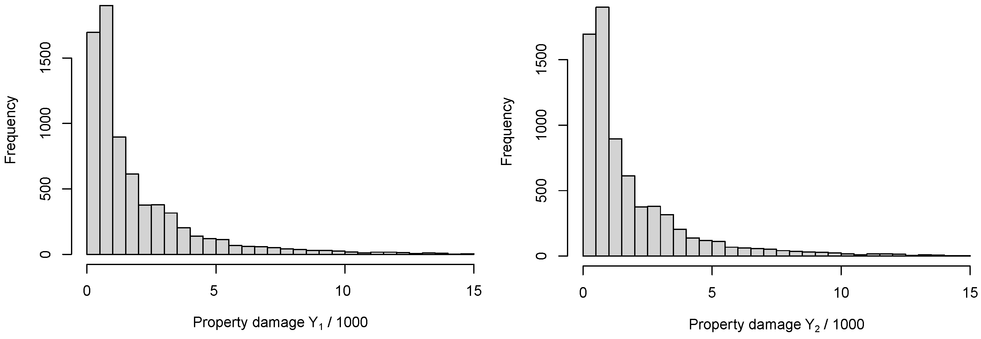
The summary statistics for $Y_1$ and $Y_2$ are shown in

Table 1. Summary statistics of two types of d claim amount. The correlation test is an one-sided test, where the alternative hypothesis is ’true correlation is greater than 0’.

Aggregated Claim	Min	Median	Mean	Max	Standard Deviation	Correlation	p-Value
$Y_1$	0.9	2413.4	11,017.3	251,958.2	27,128.85	0.1095	0.000
$Y_2$	6.2	1012.4	1871.2	14,818.2	2217.138

and Figure 1. As was expected, both $Y_1$ and $Y_2$ are positively skewed. Furthermore, the Pearson correlation test indicates that it is appropriate to model both types of claim costs based on a single bivariate model rather than two independent univariate models.

Furthermore, a description of the explanatory variables which we included in the regression analysis for $Y_1$ and $Y_2$ is provided below.

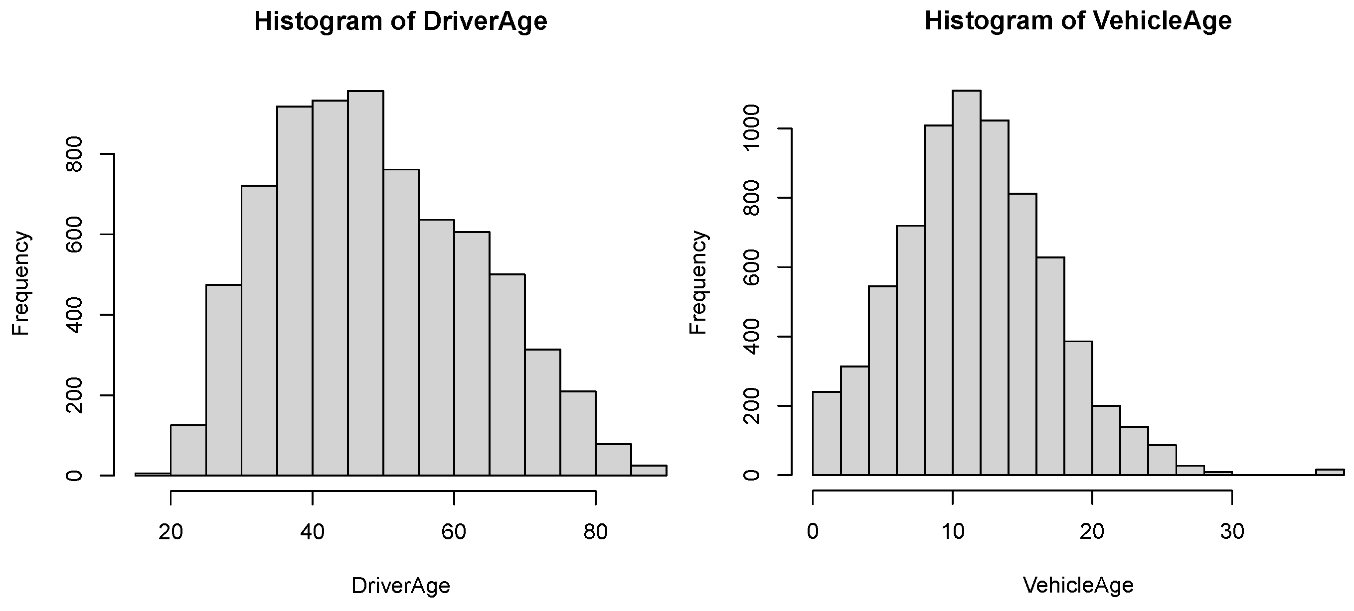
• The variable Driver’s age. Policyholders aged 18 to 90 years old.
• The variable Vehicle’s age. Vehicles aged 0 to 60 years old.
• The variable Car cubism, ’CC’, consists of four categories. Vehicles with horse power ’0–1299 cc’ (C1), ’1300–1399 cc’ (C2), ’1400–1599 cc’ and ’greater or equal 1600 cc’ (C3).
• The variable ’PT’ consisted of three types of policy, ’Economic type which includes only MTPL coverage’ (C1) , ’Middle type which includes apart from MTPL coverage other types of coverage’ (C2), and ’Expensive type—Own coverage’ (C3).
• The variable ’Region’ consisted of three board regions, ’Capital city’ (C1), ’province cities of the mainland’ (C2), and ’province cities of the island area’ (C3).

Additionally, the empirical distributions of the categorical and continuous explanatory variables are shown in

Table 2. Empirical distributions of categorical variables.

	Horse Power (CC)	Policy Type (PT)	Region
C1	2036	1144	4220
C2	2417	1940	2333
C3	1833	4179	710
C4	977	-	-

and Figure 2, respectively.

The BPA and BEIG regression models were fitted to the claim costs $\mathbf{Y}=(Y_1,Y_2)$. All computing was made using the R software. The vector of parameters $\Theta =\{{\beta }_1,{\beta }_2,\varphi \}$ was estimated using the EM algorithm which was presented in Section 3 and their standard deviations were obtained through expressions that were directly produced by the EM algorithm for the observed information matrix of each model. The fit of the competing models was compared by employing the classic hypothesis/specification tests Akaike information criterion (AIC) and Bayesian information criterion (BIC). The results are presented in

Table 3. Estimated parameters and standard errors in parentheses for the BPA and BEIG regressions model. AIC: Akaike information criterion; BIC: Bayesian information criterion.

	BPA		BEIG
Response	${\mathit{Y}}_{\mathbf{1}}$	${\mathit{Y}}_{\mathbf{2}}$	${\mathit{Y}}_{\mathbf{1}}$	${\mathit{Y}}_{\mathbf{2}}$
$\varphi$	0.5258		0.7905
	(0.0394)		(0.016)
Intercept	8.6756	8.0076	8.5108	7.8137
	(0.0979)	(0.0905)	(0.0905)	(0.0861)
Driver’s Age	0.0010	0.0028	0.0007	0.0028
	(0.0014)	(0.0012)	(0.0014)	(0.0013)
CC: C2	−0.0854	0.0761	−0.0523	0.0918
	(0.0486)	(0.0431)	(0.0481)	(0.0455)
CC: C3	0.0517	0.0661	0.0498	0.0615
	(0.0517)	(0.0463)	(0.0517)	(0.0489)
CC: C4	−0.0064	0.1104	0.0238	0.1183
	(0.0633)	(0.0564)	(0.0625)	(0.0595)
PT: C2	0.4555	−0.0352	0.3859	−0.0684
	(0.0614)	(0.0535)	(0.0599)	(0.0564)
PT: C3	0.4057	−0.0764	0.3622	−0.0989
	(0.0559)	(0.0482)	(0.0540)	(0.0506)
Vehcle’s Age	0.0155	−0.0015	0.0139	−0.0021
	(0.0035)	(0.0031)	(0.0035)	(0.0033)
Region: C2	−0.1552	0.0502	−0.1125	0.0736
	(0.0417)	(0.0369)	(0.0411)	(0.0389)
Region: C3	0.2422	−0.0306	0.2493	−0.0189
	(0.0644)	(0.0577)	(0.0643)	(0.0609)
AIC	267,937.7		267,843.1
BIC	268,082.4		267,987.8

. We see that the values of the estimated regression coefficients of the variables Driver’s Age, Vehicle’s Age and Region have a a similar effect (positive and/or negative) and are almost identical for both response variables in the case of the bivariate claim size models. Furthermore, we observe that the best fitting performances are provided by the BEIG regression models since according to a very well known rule of thumb, two models can be considered to be significantly different if the difference in their respective AIC and SBC values is greater than ten and five, respectively, see Anderson and Burnham (2004) and Raftery (1995), respectively.

Finally, we consider an extension of the proposed framework using copulas. In particular, the Gaussian copula is paired with the PA and EIG regression models. The copula-based models are compared to the BPA and BEIG regression models using two simulated datasets. The probability density functions of the univariate PA and EIG have similar definitions as those their bivariate counterparts. In particular, we have that

$$f_{PA}\left(y_{i,t}\right)=\frac{{\varphi }^{\varphi +1}(\varphi +1)}{{\mu }_{i,t}(\varphi +\frac{y_{i,t}}{{\mu }_{i,t}})},f_{EIG}\left(y_{i,t}\right)=\frac{{\varphi }^2{e}^{{\varphi }^2}}{{\mu }_{i,t}}2K_{-\frac{3}{2}}\left(\sqrt{{\varphi }^2\left({\varphi }^2+\frac{y_{i,t}}{{\mu }_{i,t}}\right)}\right){\left(\frac{{\varphi }^2}{{\varphi }^2+\frac{2y_{i,t}}{{\mu }_{i,t}}}\right)}^{\frac{3}{4}},$$

(20)

where $i=1,2$ for two marginals, $j=1,\cdots ,n$ for different policyholders and ${\mu }_{i,j}$ are the regression parameters which have the same definition as in Section 2. Two random samples of size $n=5000$ are generated from the bivariate Gaussian copula which is paired with the PA and EIG marginals, respectively. Then we consider two sets of explanatory variables ${\nu }_{1,i}-{\nu }_{4,i}$ that determine the size of ${\mu }_{i,j}$ for two marginals. In particular, we assume that ${\nu }_{1,i}$ take integer values within the ranges (18–75) and (0–20), respectively. The rest of the variables are considered to be categorical. In particular, we let ${\nu }_{2,1}$ have two categories while ${\nu }_{2,2}$ has three. Then, we consider that ${\nu }_{3,i}$ and ${\nu }_{4,i}$ have three and four categories, respectively. All the explanatory variables are generated from the uniform distribution with length n. The fitting results are shown in

Table 4. Model comparison between Gaussian copula with two PA marginals and BPA regression model. Data are generated from Gaussian copula with two PA marginals. The AIC and BIC values are for the bivariate model.

	${\mathit{Y}}_1$				${\mathit{Y}}_2$
	True	Copula with PA	BPA		True	Copula with PA	BPA
$\varphi$	2	2.0713	2.6455	$\varphi$	3	3.0353	2.6455
Intercept	−1	−1.0445	−1.0447	Intercept	−1.5	−1.5936	−1.5675
${\nu }_{1,1}$	0.0003	0.0012	0.0008	${\nu }_{1,2}$	0.003	0.0065	0.0070
${\nu }_{2,1}C2$	−0.4	−0.3527	−0.3603	${\nu }_{2,2}C2$	−0.3	−0.3182	−0.3152
${\nu }_{3,1}C2$	−0.05	0.0125	−0.0089	${\nu }_{2,2}C3$	−0.2	−0.2113	−0.2205
${\nu }_{3,1}C3$	0.1	0.0385	0.0190	${\nu }_{3,2}C2$	−0.05	−0.0329	−0.0227
${\nu }_{4,1}C2$	0.2	0.1422	0.1651	${\nu }_{3,2}C3$	0.15	0.1675	0.1628
${\nu }_{4,1}C3$	0.3	0.2438	0.2571	${\nu }_{4,2}C2$	0.25	0.2746	0.2700
${\nu }_{4,1}C4$	0.4	0.3157	0.3216	${\nu }_{4,2}C3$	0.35	0.4538	0.4366
				${\nu }_{4,2}C4$	0.45	0.5197	0.5063
$\rho$	0.2	0.1941
AIC		−4486.499	−4418.983	BIC		−4356.155	−4301.673

and

Table 5. Model comparison between Gaussian copula model with two EIG marginals and BEIG regression model. Data are generated from Gaussian copula with two EIG marginals. The AIC and BIC values are for the bivariate model.

	${\mathit{Y}}_1$				${\mathit{Y}}_2$
	True	Copula with EIG	BEIG		True	Copula with EIG	BEIG
$\varphi$	2	2.0168	2.1322	$\varphi$	3	2.7243	2.1322
Intercept	−1	−1.0676	−1.0694	Intercept	−1.5	−1.4777	−1.4709
${\nu }_{1,1}$	0.0003	0	−0.0002	${\nu }_{1,2}$	0.003	−0.0020	-0.0008
${\nu }_{2,1}C2$	−0.4	−0.3679	−0.0002	${\nu }_{2,2}C2$	−0.3	−0.2583	−0.2654
${\nu }_{3,1}C2$	−0.05	−0.0411	−0.0348	${\nu }_{2,2}C3$	−0.2	−0.1480	−0.1601
${\nu }_{3,1}C3$	0.1	0.1598	0.1676	${\nu }_{3,2}C2$	−0.05	−0.0230	−0.0279
${\nu }_{4,1}C2$	0.2	0.2485	0.2507	${\nu }_{3,2}C3$	0.15	0.1724	0.1661
${\nu }_{4,1}C3$	0.3	0.3525	0.3589	${\nu }_{4,2}C2$	0.25	0.2030	0.2083
${\nu }_{4,1}C4$	0.4	0.4232	0.4334	${\nu }_{4,2}C3$	0.35	0.3321	0.3378
				${\nu }_{4,2}C4$	0.45	0.4537	0.4450
$\rho$	0.2	0.1920
AIC		−3310.483	−3260.53	BIC		−3180.139	−3143.22

, respectively.

5. Concluding Remarks

In this paper, we developed a class of bivariate mixed Exponential regression models which can approximate moderate and large claim costs in an efficient manner based on the choice of mixing density. We illustrated our approach by fitting the BPA and BEIG regression models on MTPL data which were provided by a European insurance company. The proposed family of models can accommodate the positive correlation between MTPL bodily injury and property damage claims and their associated costs, when explanatory variables for each type of claims are taken into account through regression structure for their mean parameters.

The main achievement is that we developed an EM-type algorithm which is computationally efficient. This was demonstrated by obtaining reliable estimates when applying the models to the read data. Finally, the standard errors of estimated parameters were easily produced as byproducts of the algorithm.

References

- Abdallah, Anas, Jean-Philippe Boucher, and Hélène Cossette. 2016. Sarmanov family of multivariate distributions for bivariate dynamic claim counts model. Insurance: Mathematics and Economics 68: 120–33. [Google Scholar] [CrossRef] [Green Version]
- Anderson, David R., and Kenneth P. Burnham. 2004. Model Selection and Multi-Model Inference, 2nd ed. New York: Springer, vol. 63, p. 10. [Google Scholar]
- Bakar, S. A. Abu, Nor A. Hamzah, Mastoureh Maghsoudi, and Saralees Nadarajah. 2015. Modeling loss data using composite models. Insurance: Mathematics and Economics 61: 146–54. [Google Scholar]
- Baumgartner, Carolin, Lutz F. Gruber, and Claudia Czado. 2015. Bayesian total loss estimation using shared random effects. Insurance: Mathematics and Economics 62: 194–201. [Google Scholar] [CrossRef]
- Bermúdez, Lluís, Montserrat Guillén, and Dimitris Karlis. 2018. Allowing for time and cross dependence assumptions between claim counts in ratemaking models. Insurance: Mathematics and Economics 83: 161–69. [Google Scholar] [CrossRef]
- Bermúdez, Lluís, and Dimitris Karlis. 2011. Bayesian multivariate poisson models for insurance ratemaking. Insurance: Mathematics and Economics 48: 226–36. [Google Scholar] [CrossRef] [Green Version]
- Bermúdez, Lluís, and Dimitris Karlis. 2012. A finite mixture of bivariate poisson regression models with an application to insurance ratemaking. Computational Statistics & Data Analysis 56: 3988–99. [Google Scholar]
- Bermúdez, Lluís, and Dimitris Karlis. 2017. A posteriori ratemaking using bivariate poisson models. Scandinavian Actuarial Journal 2017: 148–58. [Google Scholar] [CrossRef] [Green Version]
- Bermúdez, Lluís, and Dimitris Karlis. 2021. Multivariate inar (1) regression models based on the sarmanov distribution. Mathematics 9: 505. [Google Scholar] [CrossRef]
- Blostein, Martin, and Tatjana Miljkovic. 2019. On modeling left-truncated loss data using mixtures of distributions. Insurance: Mathematics and Economics 85: 35–46. [Google Scholar] [CrossRef]
- Bolancé, Catalina, Montserrat Guillen, and Albert Pitarque. 2020. A Sarmanov distribution with beta marginals: An application to motor insurance pricing. Mathematics 8: 2020. [Google Scholar] [CrossRef]
- Bolancé, Catalina, and Raluca Vernic. 2019. Multivariate count data generalized linear models: Three approaches based on the Sarmanov distribution. Insurance: Mathematics and Economics 85: 89–103. [Google Scholar] [CrossRef] [Green Version]
- Calderín-Ojeda, Enrique, and Chun Fung Kwok. 2016. Modeling claims data with composite Stoppa models. Scandinavian Actuarial Journal 2016: 817–36. [Google Scholar] [CrossRef]
- Cockriel, William M., and James B. McDonald. 2018. Two multivariate generalized beta families. Communications in Statistics-Theory and Methods 47: 5688–701. [Google Scholar] [CrossRef]
- Cooray, Kahadawala, and Malwane M. A. Ananda. 2005. Modeling actuarial data with a composite lognormal-Pareto model. Scandinavian Actuarial Journal 2005: 321–34. [Google Scholar] [CrossRef]
- Denuit, Michel, Montserrat Guillen, and Julien Trufin. 2019. Multivariate credibility modelling for usage-based motor insurance pricing with behavioural data. Annals of Actuarial Science 13: 378–99. [Google Scholar] [CrossRef] [Green Version]
- Frees, Edward W. 2009. Regression Modeling with Actuarial and Financial Applications. Cambridge: Cambridge University Press. [Google Scholar]
- Fung, Tsz Chai, Andrei L. Badescu, and X. Sheldon Lin. 2019. A class of mixture of experts models for general insurance: Application to correlated claim frequencies. ASTIN Bulletin: The Journal of the IAA 49: 647–88. [Google Scholar] [CrossRef]
- Fung, Tsz Chai, Andrei L. Badescu, and X. Sheldon Lin. 2021. A new class of severity regression models with an application to ibnr prediction. North American Actuarial Journal 25: 206–31. [Google Scholar] [CrossRef]
- Gómez-Déniz, Emilio, and Enrique Calderín-Ojeda. 2021. A priori ratemaking selection using multivariate regression models allowing different coverages in auto insurance. Risks 9: 137. [Google Scholar] [CrossRef]
- Grün, Bettina, and Tatjana Miljkovic. 2019. Extending composite loss models using a general framework of advanced computational tools. Scandinavian Actuarial Journal 2019: 642–60. [Google Scholar] [CrossRef]
- Jeong, Himchan, and Dipak K. Dey. 2021. Multi-Peril Frequency Credibility Premium via Shared Random Effects. Available online: https://papers.ssrn.com/sol3/papers.cfm?abstract_id=3825435 (accessed on 13 April 2021).
- Jeong, Himchan, and Emiliano A. Valdez. 2020. Predictive compound risk models with dependence. Insurance: Mathematics and Economics 94: 182–95. [Google Scholar] [CrossRef]
- Laudagé, Christian, Sascha Desmettre, and Jörg Wenzel. 2019. Severity modeling of extreme insurance claims for tariffication. Insurance: Mathematics and Economics 88: 77–92. [Google Scholar] [CrossRef]
- Lee, Simon C. K., and X. Shelson Lin. 2010. Modeling and evaluating insurance losses via mixtures of Erlang distributions. North American Actuarial Journal 14: 107–30. [Google Scholar] [CrossRef]
- Miljkovic, Tatjana, and Bettina Grün. 2016. Modeling loss data using mixtures of distributions. Insurance: Mathematics and Economics 70: 387–396. [Google Scholar] [CrossRef]
- Nadarajah, Saralees, and S. A. Abu Bakar. 2014. New composite models for the Danish fire insurance data. Scandinavian Actuarial Journal 2014: 180–87. [Google Scholar] [CrossRef]
- Oh, Rosy, Himchan Jeong, Jae Youn Ahn, and Emiliano A. Valdez. 2021. A multi-year microlevel collective risk model. Insurance: Mathematics and Economics 100: 309–28. [Google Scholar] [CrossRef]
- Parodi, Pietro. 2020. A generalised property exposure rating framework that incorporates scale-independent losses and maximum possible loss uncertainty. Astin Bulletin 50: 513–53. [Google Scholar] [CrossRef]
- Pechon, Florian, Michel Denuit, and Julien Trufin. 2019. Multivariate modelling of multiple guarantees in motor insurance of a household. European Actuarial Journal 9: 575–602. [Google Scholar] [CrossRef] [Green Version]
- Pechon, Florian, Michel Denuit, and Julien Trufin. 2021. Home and motor insurance joined at a household level using multivariate credibility. Annals of Actuarial Science 15: 82–114. [Google Scholar] [CrossRef]
- Pechon, Florian, Julien Trufin, and Michel Denuit. 2018. Multivariate modelling of household claim frequencies in motor third-party liability insurance. Astin Bulletin 48: 969–93. [Google Scholar] [CrossRef] [Green Version]
- Pigeon, Mathieu, and Michel Denuit. 2011. Composite lognormal-Pareto model with random threshold. Scandinavian Actuarial Journal 2011: 177–92. [Google Scholar] [CrossRef]
- Raftery, Adrian E. 1995. Bayesian model selection in social research. Sociological Methodology 25: 111–163. [Google Scholar] [CrossRef]
- Reynkens, Tom, Roel Verbelen, Jan Beirlant, and Katrien Antonio. 2017. Modelling censored losses using splicing: A global fit strategy with mixed Erlang and extreme value distributions. Insurance: Mathematics and Economics 77: 65–77. [Google Scholar] [CrossRef] [Green Version]
- Scollnik, David P. M. 2007. On composite lognormal-Pareto models. Scandinavian Actuarial Journal 2007: 20–33. [Google Scholar] [CrossRef]
- Scollnik, David P. M., and Chenchen Sun. 2012. Modeling with Weibull-Pareto models. North American Actuarial Journal 16: 260–72. [Google Scholar] [CrossRef]
- Shi, Peng, and Emiliano A. Valdez. 2014a. Longitudinal modeling of insurance claim counts using jitters. Scandinavian Actuarial Journal 2014: 159–79. [Google Scholar] [CrossRef]
- Shi, Peng, and Emiliano A. Valdez. 2014b. Multivariate negative binomial models for insurance claim counts. Insurance: Mathematics and Economics 55: 18–29. [Google Scholar] [CrossRef]
- Tzougas, George, and Alice Pignatelli di Cerchiara. 2021a. Bivariate mixed poisson regression models with varying dispersion. North American Actuarial Journal, 1–31. [Google Scholar] [CrossRef]
- Tzougas, George, and Alice Pignatelli di Cerchiara. 2021b. The multivariate mixed negative binomial regression model with an application to insurance a posteriori ratemaking. Insurance: Mathematics and Economics 101: 602–25. [Google Scholar] [CrossRef]
- Tzougas, George, and Himchan Jeong. 2021. An expectation-maximization algorithm for the exponential-generalized inverse gaussian regression model with varying dispersion and shape for modelling the aggregate claim amount. Risks 9: 19. [Google Scholar] [CrossRef]
- Tzougas, George, and Dimitris Karlis. 2020. An em algorithm for fitting a new class of mixed exponential regression models with varying dispersion. Astin Bulletin 50: 555–83. [Google Scholar] [CrossRef]
- Tzougas, George, Spyridon Vrontos, and Nicholas Frangos. 2014. Optimal bonus-malus systems using finite mixture models. Astin Bulletin 44: 417–44. [Google Scholar] [CrossRef] [Green Version]
- Tzougas, George, Spyridon Vrontos, and Nicholas Frangos. 2018. Bonus-malus systems with two-component mixture models arising from different parametric families. North American Actuarial Journal 22: 55–91. [Google Scholar] [CrossRef]
- Yang, Xipei, Edward W. Frees, and Zhengjun Zhang. 2011. A generalized beta copula with applications in modeling multivariate long-tailed data. Insurance: Mathematics and Economics 49: 265–84. [Google Scholar] [CrossRef]
Figure 1.
Empirical distribution of two types of d claim amount.
Figure 2.
Empirical distributions of continuous explanatory variables.