Practice Oriented and Monte Carlo Based Estimation of the Value-at-Risk for Operational Risk Measurement

Abstract

We explore the Monte Carlo steps required to reduce the sampling error of the estimated 99.9% quantile within an acceptable threshold. Our research is of primary interest to practitioners working in the area of operational risk measurement, where the annual loss distribution cannot be analytically determined in advance. Usually, the frequency and the severity distributions should be adequately combined and elaborated with Monte Carlo methods, in order to estimate the loss distributions and risk measures. Naturally, financial analysts and regulators are interested in mitigating sampling errors, as prescribed in EU Regulation 2018/959. In particular, the sampling error of the 99.9% quantile is of paramount importance, along the lines of EU Regulation 575/2013. The Monte Carlo error for the operational risk measure is here assessed on the basis of the binomial distribution. Our approach is then applied to realistic simulated data, yielding a comparable precision of the estimate with a much lower computational effort, when compared to bootstrap, Monte Carlo repetition, and two other methods based on numerical optimization.

1. Introduction

International financial institutions typically calculate capital requirements for operational risk via the advanced measurement approach (AMA). The AMA is based on statistical models that are internally defined by institutions and comply with regulatory requirements (see European Parliament and Council of the European Union 2013). In particular, the regulations define which data sources must be used to measure operational risk:

• internal loss data;
• external loss data;
• scenario analysis; and
• business environmental and internal control factors.

Another significant requirement specifies that the capital charge has to be calculated at the 99.9% confidence level, with the holding period of one year. This means that the financial institution may experience an annual loss higher than the capital requirement once every 1000 years, on average.

The most-adopted implementation of AMA models is the loss distribution approach (see Frachot et al. 2001, 2007), where the objective is to estimate the probability distribution of the annual loss amount. In more detail, the loss data is categorized by Operational Risk Categories (ORCs), such that the independent and identical distribution (iid) hypothesis is applicable within each ORC. For each ORC, the severity distribution (i.e., the probability distribution of a single loss amount) and the frequency distribution (i.e., the probability distribution of the number of losses in one year) are estimated. The annual loss distribution for each ORC is obtained through a convolution process, and practically implemented with approximation or numerical techniques, since it is not usually feasible to represent the convolution function in closed form. For this aim, the main available approaches are:

• Monte Carlo method,
• Fourier transform-related methods,
• Panjer algorithm, and
• single loss approximation.

Naturally, these methodologies have their pros and cons, which have to be carefully considered when they are adopted. In particular:

• Monte Carlo method (see Owen 2013) is the most flexible and widely used technique, but it requires intensive computations and converges slowly to the correct result. In particular, the sampling error decreases proportionally to the square root of the number of steps.
• Fourier transform-related methods and the Panjer algorithm (see Klugman et al. 2012; Embrechts and Frei 2009) allow for a higher accuracy based on less intensive computations, but they require to carefully define the discretization of the severity distribution, to avoid underflow or overflow cases. The complexity of a valid discretization for the severity distribution has, usually, limited the usage of these techniques in the AMA models. In fact, while the slow convergence of the Monte Carlo method can affect the accuracy of the estimates, the underflow or overflow cases can potentially lead to totally unrealistic results.
• Single loss approximation (SLA) (see Böcker and Klüppelberg 2005; Böcker and Sprittulla 2006) allows approximating a high level quantile (corresponding to a probability close to 1) of the annual loss distribution on the basis of a particular quantile of the severity distribution and of the average of the frequency distribution. In particular, the SLA says that the 99.9% quantile of the annual loss distribution G can be approximated by the quantile of the severity distribution F at the level $1-(1-0.999)/\lambda$, where $\lambda$ is the average of the frequency distribution, i.e., $G^{-1}\left(0.999\right)\approx F^{-1}(1-(1-0.999)/\lambda )$. Therefore, the shape of the frequency distribution does not significantly affect the 99.9% quantile of the loss distribution. This technique is very useful to obtain a quick proxy for the 99.9% quantile of the annual loss distribution but, being an asymptotic result, it is valid only for high level quantiles and cannot be used to define the entire annual loss distribution.

As suggested by the SLA, the purpose of AMA models is to estimate the severity distribution. This calculation phase of the AMA models is heavily affected by the “extrapolation issue” (see Mignola and Ugoccioni 2006; Cope et al. 2009). In fact, since the 99.9% quantile of the annual loss distribution approximately corresponds to the $1-(1-0.999)/\lambda$ quantile of the severity distribution, this means that $\lambda /(1-0.999)=\lambda /0.001=1000\lambda$ losses would be needed to estimate the 99.9% quantile of the annual loss distribution without resorting to extrapolation. This is because, in order to calculate the quantile of probability p (where $0<p<1$) without extrapolation, we need at least $1/(1-p)$ data. In recent years, banks have been collecting data, besides reporting current losses, and an effort has been made to build data bases going back in time. In any case, no more than ten to fifteen years of loss data are available, and so the capital requirement needs a delicate extrapolation. To extrapolate beyond the data, therefore, parametric models for the severity distribution can be applied. In fact, non-parametric estimation does not provide any guidance outside of the range of observed data. Usually, parametric models are applied only above a sufficiently high loss threshold to fit the tail of the severity distribution; while the losses below the threshold (i.e., the body of the severity distribution) can be easily modeled using non-parametric methods, e.g., the empirical distribution. The lognormal, loglogistic, Weibull, Pareto and generalized Pareto are among the most common model choices (see Bolancel et al. 2012; Klugman et al. 2012). The parameters (e.g., $(\mu ,\sigma )$ for the lognormal distribution) can be estimated through the maximum likelihood method, adopting truncated or shifted distributions (see Cavallo et al. 2012; Luo et al. 2007) to fit the models above a specified threshold.

Many other methods have been proposed to reduce the issues due to the extrapolation, among them are the following ones:

• Internal loss data are complemented with external loss data and a scenario analysis in the estimation of the severity distributions. Such an integration can be coherently performed using Bayesian methods (see Lambrigger et al. 2007; Shevchenko 2011; Dalla Valle and Giudici 2008; Figini et al. 2014; Shevchenko and Wüthrich 2006).
• Robust methods are employed to yield model parameters, like the weighted likelihood or the Optimal B-Robust estimation method (see Colombo et al. 2015; Danesi and UniCredit Business Integrated Solutions 2015; Danesi et al. 2016, respectively).

The AMA methods usually incorporate a fitting procedure to select the best model and threshold (i.e., tail parametric model) for each ORC (see Chernobai et al. 2005; Lavaud and Leherisse 2014; Panjer 2006). It has to be noted that a sound procedure to select the best tail model should include measures of both the goodness-of-fit vs loss data and the uncertainty of the estimated capital requirement (see Larsen 2016, 2019).

Whenever the shape of the frequency distribution does not significantly affect the capital requirement, as it has been discussed in the SLA approach, then the frequency distribution is estimated through the simplest possible model, which is the Poisson distribution. This discrete probability distribution has only one parameter $\lambda$, representing both the average and the variance of the number of loss data in one year. Once, for each ORC, the severity and the frequency distributions have been estimated, the annual loss distribution can be approximated through one of the above mentioned techniques, e.g., the Monte Carlo method. Starting with the annual loss distributions of the ORCs as margins, the overall annual loss distribution is usually obtained by applying a copula function. In fact, on the basis of Sklar’s theorem, if F is an n-dimensional cdf with continuous margins $F_1,\dots ,F_n$, then it has the unique copula representation $F(x_1,\dots ,x_n)=C(F_1\left(x_1\right),\dots ,F_n\left(x_n\right))$, where C is the copula function, i.e., a multivariate cdf with margins uniformly distributed on [0,1], with the following properties:

• $C:{[0,1]}^n\to [0,1]$;
• C is grounded, i.e., $C_i\left(u\right)=C(u_1,\dots ,u_{i-1},0,u_{i+1},\dots ,u_n)=0$ for all $i=1,\dots ,n$, and n-increasing;
• C has margins $C_i(i=1,\dots ,n)$ satisfying $C_i\left(u\right)=C(1,\dots ,1,u,1,\dots ,1)=u$ for all $u\in [0,1]$.

In practice, we see that for continuous multivariate distribution functions, the univariate margins and the multivariate dependence structure can be separated. The dependence structure can be represented by a proper copula function, e.g., the Student t-copula (see Di Clemente and Romano 2004). The capital requirement is then, usually, defined through the Value-at-Risk (VaR) measure, as the 99.9% quantile of the overall annual loss distribution. Deductions for insurance (see Bazzarello et al. 2006) and expected losses are often considered in AMA models. For expected loss deduction, the European Parliament and Council of the European Union (2013) states that a financial institution shall calculate its capital requirement for operational risk as comprising both the expected loss and the unexpected loss, unless the expected loss is adequately captured in its internal business practices. We can see the 99.9% quantile of the overall annual loss distribution as the sum between the expected loss and the unexpected loss, from which the expected loss could be eventually deducted. To obtain this deduction, it is necessary to comply with the requirements reported in European Parliament and Council of the European Union (2018):

• the expected loss estimation process is done by ORC and is consistent over time;
• the expected loss is calculated using statistics that are less influenced by extreme losses, including median and trimmed mean, especially in the case of medium- or heavy-tailed data;
• the maximum offset for expected loss applied by the institution is bounded by the total expected loss;
• the maximum offset for expected loss in each ORC is bound by the relevant expected losses calculated according to the institution’s operational risk measurement system applied to that category;
• the offsets the institution allows for expected loss in each ORC are capital substitutes or available to cover expected loss with a high degree of certainty (e.g., provisions) over the one-year period;
• specific reserves for exceptional operational risk loss events, that have already occurred, cannot be used as expected loss offsets.

In case the annual loss distributions for the ORCs and the related overall annual loss distribution are obtained through the Monte Carlo method, such distributions have to be represented by a sufficiently high number of simulated data. Following the terminology adopted by the EU regulators, the number of Monte Carlo steps refers to the sample size. For example, with 5 million data points, the $99.9\%$ quantile can be estimated via the empirical estimator as the value at position 4,995,000 in the increasing ordered sequence of the simulated losses. It provides the capital requirement for operational risk.

2. The Monte Carlo Method: An Introduction

The Monte Carlo method has a long history in statistics, where it was also called ‘model sampling’. It was used to verify the properties of estimates by reproducing the settings for which they were designed. W. S. Gosset, writing as Student (1908), before deriving analytic result on Student’s t distribution, did some simulations, using height and left middle finger measurements from 3000 criminals as written on pieces of cardboard. Additional history on the Monte Carlo method can be found in Kalos and Whitlock (2008) including computations made by Fermi in the 1930s. This method became more important in the 1940s and early 1950s, when it was also used to solve problems in physics, related to atomic weapons. The name itself was assigned in this period, taken from the famous casino located in Monte Carlo.

There are several papers in which the Monte Carlo method is widely used for new problems. For example, Metropolis et al. (1953) presented the Metropolis algorithm, which was the first Markov chain Monte Carlo method. Boyle (1977) showed how to apply Monte Carlo methods to financial options pricing. Efron (1979) defined the bootstrap, using Monte Carlo method to derive statistical properties without specifying distributional assumptions.

Approximately during the same period, the Quasi-Monte Carlo techniques were defined. The term itself was assigned by Richtmyer (1952). He thought to improve Monte Carlo by using sequences with better uniformity than truly random sequences would have.

The uniform distribution on $[0,1]$ is fundamental in the theory of Monte Carlo method. In fact the simulation methods derive their randomness from sequences of independent, uniformly distributed, random variables on $[0,1]$. A continuous random variable U is uniformly distributed on $[0,1]$ if it has the following probability density function

$$f_U\left(u\right)=\left\{\begin{array}{cc}1,\hfill & \mathrm{if}u\in [0,1];\hfill \\ 0,\hfill & \mathrm{otherwise}.\hfill \end{array}\right.$$

(1)

In order to generate a realization from a non-uniform distribution, random numbers uniformly distributed on $[0,1]$ can be transformed in observations extracted from the desired distribution. Given a random variable X, its cumulative distribution function $F_X\left(x\right)$ is an increasing function on $[0,1]$. If $F_X\left(x\right)$ is continuous and strictly increasing (i.e., $F_X\left(x_1\right)<F_X\left(x_2\right)$ if $x_1<x_2$), then it assumes all the values between 0 and 1. In this case, the inverse function $F_X^{-1}\left(y\right)$ (i.e., the quantile function) can be defined, such that $y=F_X\left(x\right)$⟺$x=F_X^{-1}\left(y\right)$. More generally, the quantile function can be defined as $F_X^{-1}\left(y\right)=\inf \{x:F_X\left(x\right)\ge y\}$. Hence, to obtain a random number c from a random variable X, one can generate a number r from the uniform distribution on $[0,1]$ and calculate $c=F_X^{-1}\left(r\right)$.

Actually, no sequence generated through an algorithm, and hence through a computer, can be really considered ‘random’. In fact, we can only generate sequences of pseudo-random numbers, i.e., numbers which are apparently random. A pseudo-random sequence is built by a sequence of values $x_j$, for which the first k values $x_0,x_1,\dots ,x_{k-1}$ are chosen, and each of the next values $x_j$, $j\ge k$ is obtained by applying a function on the k previous values $x_{j-1},x_{j-2},\dots ,x_{j-k}$. The sequence of the first k values $x_0,x_1,\dots ,x_{k-1}$ is named ‘seed’. Therefore, the entire sequence of generated numbers depends on the value of the seed. Generally, the generation of random sequences is based on a linear congruential generator defined as follows

$$x_{j+1}=(a·x_j+b)\mathrm{mod}m$$

(2)

where a is the multiplier, b is the shift, and m is the module. The best of these quickly produce very long streams of numbers, and have fast and portable implementations in many programming languages. Among these high quality generators, the Mersenne twister, MT19937, of Matsumoto and Nishimura (1998) has become the most prominent, though it is not the only high quality random number generator. We also cite the ‘combined multiple-recursive generator’ from L’Ecuyer (1999).

In a simple Monte Carlo problem (see Owen 2013) we define the quantity to be estimated as the expected value of a random variable Y, i.e., $\mu =\mathbb{E}\left(Y\right)$. Please note that the estimation of average is the most basic application of Monte Carlo method, which is generally used to introduce the approach. The estimation of quantile, which is of main interest in operational risk measurement, will be discussed from the following sections. To begin with, we generate values $Y_1,\dots ,Y_n$ independently and randomly from the distribution of Y and take their average

$${\widehat{\mu }}_n=\frac{1}{n}\sum _{i=1}^n{Y}_i$$

(3)

as the estimate of $\mu$. Usually, we have $Y=f\left(X\right)$ where the random variable $X\in D\subset {\mathbb{R}}^d$ has a probability density function $p\left(x\right)$, and f is a real-valued function defined over D. Then $\mu ={\int }_{D}f\left(x\right)p\left(x\right)dx$.

The simple Monte Carlo is justified through the laws of large numbers, assuring that under simple conditions ($\mu$ has to exist), the sample-average estimator converges to the actual value. This tells us that Monte Carlo will eventually produce an error as small as we like, but it does not tell us how large n has to be for this to happen. Supposing that Y has a finite variance (${\sigma }^2<\infty$), ${\widehat{\mu }}_n$ is a random variable having mean

$$\mathbb{E}\left({\widehat{\mu }}_n\right)=\frac{1}{n}\sum _{i=1}^n\mathbb{E}\left(Y_i\right)=\mu ,$$

(4)

and variance

$$\mathbb{E}\left({({\widehat{\mu }}_n-\mu )}^2\right)=\frac{{\sigma }^2}{n}.$$

(5)

Therefore, the standard deviation of ${\widehat{\mu }}_n$ is equal to $\sqrt{\mathbb{E}\left({({\widehat{\mu }}_n-\mu )}^2\right)}=\frac{\sigma }{\sqrt{n}}$. This means that to get one more decimal digit of accuracy is equivalent to asking for a standard deviation one tenth as large, and that requires a 100-fold increase in computation. The value of ${\sigma }^2$ can be estimated by

$$s^2=\frac{1}{n-1}\sum _{i=1}^n{(Y_i-{\widehat{\mu }}_n)}^2.$$

(6)

The variance estimate $s^2$ tells us that the standard error is of the order of $s/\sqrt{n}$. From the central limit theorem (CLT), we also know that ${\widehat{\mu }}_n-\mu$ has approximately a normal distribution with mean 0 and variance $s^2/n$. This yields the familiar 95% confidence interval

$${\widehat{\mu }}_n-1.96\frac{s}{\sqrt{n}}\le \mu \le {\widehat{\mu }}_n-1.96\frac{s}{\sqrt{n}}.$$

(7)

Since the Monte Carlo method typically has an error variance of the form $\frac{{\sigma }^2}{n}$, we get a more accurate estimate by sampling with a larger value of n. However, the computing time grows with n. Therefore several techniques have been defined to reduce $\sigma$ (see Owen 2013; Kleijnen et al. 2010). To do this, new Monte Carlo methods can be constructed, having the same answer as the simple one but with a lower $\sigma$. These methods are known as variance reduction techniques:

• Antithetic sampling: let $\mu =\mathbb{E}\left(X\right)$ for $X\sim p$, where p is a symmetric density on the symmetric set D. Here, symmetry is with respect to reflection through the center point of D. If we reflect $x\in D$ through c we get the point $\tilde{x}$ with $\tilde{x}-c=-(x-c)$, that is $\tilde{x}=2c-x$. Symmetry means that $p\left(\tilde{x}\right)=p\left(x\right)$ including the constraint that $x\in D$ if and only if $\tilde{x}\in D$. The antithetic sampling estimate of $\mu$ is

  $${\widehat{\mu }}_{anti}=\frac{1}{n}\sum _{i=1}^{n/2}(f\left(X_i\right)+\tilde{f}\left(X_i\right)),$$

  (8)

  where $X_i\sim p$, and n is an even number. It can be proved that the variance in antithetic sampling is

  $$Var\left({\widehat{\mu }}_{anti}\right)=\frac{{\sigma }^2}{n}(1+\rho ),$$

  (9)

  where $\rho =Corr(f\left(X\right);\tilde{f}\left(X\right))$. From $-1\le \rho \le 1$ we obtain $0\le {\sigma }^2(1+\rho )\le 2{\sigma }^2$. In the best case, antithetic sampling gives the exact answer from just one pair of function evaluations. In the worst case it doubles the variance. Both cases do arise. It is clear that a negative correlation is favorable.
• Stratification: the idea in stratified sampling is to split up the domain D of X into separate regions, take a sample of points from each such region, and combine the results to estimate $\mathbb{E}\left(f\right(X\left)\right)$. Intuitively, if each region gets its fair share of points then we should get a better answer. One might be able to do better still by oversampling within the important strata and undersampling those in which f is nearly constant.
• Common Random Numbers (CRN): this technique applies when we are comparing two or more alternative configurations (of a system) instead of investigating a single configuration. CRN requires synchronization of the random number streams, which ensures that in addition to using the same random numbers to simulate all configurations, a specific random number used for a specific purpose in one configuration is used for exactly the same purpose in all other configurations.
• Control variate: control variates provide ways to exploit closed form results. With control variates we use some other problems, quite similar to our given one, but for which an exact answer is known. The precise meaning of ’similar’ depends on how we use this other problem, and more than one method is given below. As for ’exact’, we mean it literally, but in practice it may just mean known with an error negligible when compared to Monte Carlo errors.
• Importance sampling: the idea behind importance sampling is that certain values of the input random variables in a simulation have more impact on the parameters being estimated than others. If these ‘important’ values are sampled more frequently, then the variance can be reduced. The basic methodology in importance sampling is to choose a distribution which ‘encourages’ the important values. This use of ‘biased’ distributions will result in a biased estimator, if it is applied directly in the simulation. However, if the simulation outputs are weighted to correct for the use of the biased distribution, this will ensure that the new importance sampling estimator is unbiased. The weight is given by the likelihood ratio, that is, the Radon–Nikodym derivative of the true underlying distribution with respect to the biased simulation distribution. The fundamental issue in implementing importance sampling is the choice of a biased distribution which encourages the important regions of the input variables. Choosing a good biased distribution is the core part of importance sampling. The rewards for a good distribution can be huge run-time savings; the penalty for a bad distribution can be longer run times than for a simple Monte Carlo simulation without importance sampling.

We also mention the Quasi-Monte Carlo methods, which use low-discrepancy sequences (also called quasi-random sequences or sub-random sequences). This is in contrast to the simple Monte Carlo method, which is based on sequences of pseudorandom numbers. The advantage of using low-discrepancy sequences is a faster rate of convergence. Quasi-Monte Carlo has a rate of convergence of order $1/n$, whereas—as already mentioned above—the rate for the simple Monte Carlo method is $1/\sqrt{n}$.

In this paper we treat and apply the simple Monte Carlo method, which is also known as crude Monte Carlo to distinguish it from more sophisticated methods. In fact, all of the more sophisticated methods offer several promising technical venues for implementing the capital requirement estimation methods that we discuss. However, we have chosen the simple method because we have found it to be the easiest to be applied by practitioners working in the industry, where simplicity is often preferred to more complex methods. Moreover, calculations with simple Monte Carlo method can be easily distributed to more CPUs, allowing for a parallel computation, in order to make them less time consuming. In fact, most of adopted softwares in statistics offer built-in routines for parallel computations (e.g., parallel package in R by R Core Team (2016)), allowing reducing the calculation time of simple Monte Carlo proportionally to the number of used CPUs.

3. The Monte Carlo Method: Basic Definitions for Operational Risk Measurement

As mentioned in Section 1, Monte Carlo simulations are widely employed in the operational risk measurement. A detailed description of the Monte Carlo method applied to the calculation of annual loss distribution and capital requirement for operational risk can be found in Guharay et al. (2016). Here we will recall briefly the main idea behind it.

Let S be the random variable defined as

$$S=\sum _{i=1}^N{X}_i$$

(10)

describing the annual loss distribution, where $X_i$ is the random variable representing the severity of the i-th operational risk loss event, and N is the random variable representing the number of single operational risk loss events, for each year. On the basis of the above notation, the Monte Carlo method can be implemented by executing the following sequence of instructions at the generic step j:

• from the frequency distribution, draw a value $n_j$ representing the number of loss events for year j;
• from the severity distribution, draw the amounts $x_{1j},\dots ,x_{n_{j}j}$ of loss events;
• calculate the annual loss amount for year j, that is $s_j={\sum }_{i=1}^{n_j}{x}_{ij}$;

and iterate the above three steps for a sufficiently large number J of steps. The capital requirement can be evaluated as the empirical $99.9\%$ quantile of the simulated sample of the annual losses $s_1,s_2,\dots ,s_J$. In practice, after ordering the sequence ${\left\{s_j\right\}}_{j=1,\dots ,J}$ to obtain $s_{1:J}\le s_{2:J}\le \dots \le s_{J:J}$, the capital requirement corresponds to the annual loss $s_{j:J}$ with $j=99.9\%J$.

It is well known (as already mentioned in Section 2) that the sampling accuracy of the capital requirement, calculated through the Monte Carlo method, increases proportionally to the square root of the number of steps (see Owen 2013). In other words, increasing the number of steps by 100 times, the random sampling error is expected to decrease by 10 times. Therefore, when the annual loss distribution and the related 99.9% quantile are approximated by the Monte Carlo method, the good practice would require to consider and, possibly, measure the consequent sampling error. Moreover, the recently published EU Regulatory Technical Standards (European Parliament and Council of the European Union 2018) require that irrespective of the techniques adopted to obtain the annual loss distribution and the related 99.9% quantile, the institution adopts criteria that mitigate sampling and numerical errors and provides a measure of their magnitude. With reference to the Monte Carlo method, the Regulatory Technical Standards 2018/959 require that:

• the number of steps to be performed is consistent with the shape of the distributions and with the confidence level to be achieved;
• where the distribution of losses is heavy-tailed and measured at a high confidence level, the number of steps is sufficiently large to reduce sampling variability below an acceptable threshold.

To comply with these requirements, the sampling variability, i.e., the random sampling error, has to be assessed. Having estimated such an error, given the acceptable threshold (reasonably defined in terms of a low percentage of the 99.9% quantile), it is possible to verify whether the number of steps is sufficiently large and, consequently, consistent with the shape of the estimated distribution. It is worth mentioning that the topic of the sampling error related to the Monte Carlo method is also considered by Mignola and Ugoccioni (2006), based on the previous work of Chen and Kelton (2001).

There is a discussion in the recent literature on extreme quantile estimation and the adoption of some types of Monte Carlo techniques, as in Boos (1984); Danielsson and De Vries (1996); Peng and Qi (2006); Gomes and Pestana (2007). The proposed methodologies are mainly based on the Extreme Value Theory (EVT). However, in the operational risk measurement context, the EVT is no longer intensively used by practitioners, despite its interesting theoretical properties. In fact, when the EVT is applied to actual operational risk data, several practical problems arise, due to the failure of achieving the asymptotic regime described by the theory. Additionally, the capital requirement measures based on EVT are affected by the high volatility due to the use of Pareto-type tails (see Mignola and Ugoccioni 2005; Makarov 2006). In any case, EVT methods can be conjugated with the present approach, but such development is beyond the scope and purpose of this paper—it can be an interesting topic for further studies.

4. The Monte Carlo Error in Operational Risk Measurement

Suppose that using Monte Carlo techniques applied to historical data, we have obtained a set of n losses, which are positive real numbers, assuming that we do not take into account null values for losses. Hence, we are dealing with outcomes of n positive i.i.d. random variables (rv’s)

$$X_1,X_2,\dots ,X_n$$

(11)

with cdf $F\left(x\right)$ and quantile function $F^{-1}\left(p\right)$. The focus of actuaries is on large losses, and thus on large order statistics of the $Xs$. In this framework, percentiles are rich informative measures that can be represented using the order statistics $X_{1:n}\le X_{2:n}\le \dots \le X_{n:n}$ of rv’s (11). From the mathematical point of view, by ordering rv’s we obtain a monotone sequence and thus extract additional information from the original rv’s (11). In a general setting, we want to obtain a confidence interval for $VaR\left(p\right)=F^{-1}\left(p\right)$, for some p in (0,1), but the focus here is to measure the error when estimating a very high (an extreme) quantile $F^{-1}\left(p\right)$, say for $p=0.999$ for the operational risk measurement. Once we have a CI, we can define:

• the Monte Carlo error (E) as the width of the CI, and
• the relative Monte Carlo error (RE) as the ratio between the width of the CI and the best available estimate of the 99.9% quantile itself.

To construct a CI, we consider (and compare) the following methods:

• the method based on the binomial distribution applied on the quantile, as proposed by Owen (2013);
• the bootstrap (or re-sampling) method (i.e., the classical n-bootstrap and the m-out-of-n-bootstrap), where we get the probability distribution of the 99.9% quantile by drawing random samples with replacement from the annual loss distribution generated by the Monte Carlo method;
• the Monte Carlo repetition method, where we simulate the probability distribution of the 99.9% quantile, repeating several times the Monte Carlo method;
• two methods based on constrained optimization.

Since we suppose that the severity and the frequency distributions are already known or, in any case, already estimated, some typical operational risk distribution functions and parameterizations can be considered, in order to run the above mentioned methods and to analyze results. In particular, the lognormal pdf

$$f_X\left(x\right)=\frac{1}{x\sigma \sqrt{2\pi }}\exp \left(-\frac{{(\ln x-\mu )}^2}{2{\sigma }^2}\right),$$

$\mathrm{for}x>0,\mathrm{with}-\infty <\mu <+\infty \mathrm{and}\sigma >0$, can be used to model the severity (with, e.g., parameters $\mu =9$ and $\sigma =2$), and the Poisson distribution can be used to model the frequency (with, e.g., parameter $\lambda =100$, i.e., assuming 100 losses per year, on average). Such choices are motivated by previous works in the literature; see, for example, Frachot et al. (2001, 2007); Mignola and Ugoccioni (2005); Böcker and Sprittulla (2006).

Naturally, other models can be adopted for the severity distribution. We may for example consider, as a valuable alternative, the three-and four-parameter lognormal distributions, or gamma-type, or beta-type, or Pareto-type size distributions (see Kleiber and Kotz (2003) for a detailed review). Recent papers on thick-tailed distributions have adopted a semi-nonparametric approach (the so-called log-SNP, see, e.g., Cortés et al. (2017)) that generalizes the lognormal incorporating not only thick tails but also non-monotonic decay, multimodality and many other salient empirical features of the distribution of losses. This approach presents a valuable avenue for future research on operational risk.

For simplicity, we suppose that the overall annual loss distribution is generated on the basis of a single ORC, without affecting the generality of our results. Therefore, applying the Monte Carlo method, we simulate a sample of $n=5$ million annual losses. We obtain the estimated $99.9\%$ quantile as $VaR\left(0.999\right)=47.8037\times {10}^6$, and we are now ready to evaluate the different CIs for the latter.

4.1. The Binomial Distribution Method

To begin with, we employ the approach based on the binomial distribution (see Owen 2013). The idea behind this method is that the number of simulated annual losses below the 99.9% quantile follows the binomial distribution $B_{n,\theta }$, where n is the number of simulated annual losses and $\theta =0.999$.

Let S have a continuous distribution. Then $\mathbb{P}(S\le Q^{\theta })=\theta$ holds and so $Q^{\theta }=\eta$ if and only if $\mathbb{E}\left({\mathbb{1}}_{S\le \eta }\right)=\theta$. If $\theta$ is not included in the confidence interval for $\mathbb{E}\left({\mathbb{1}}_{S\le \eta }\right)$, then we can reject $Q^{\theta }=\eta$. As a result, we can obtain confidence intervals for $Q^{\theta }$ using confidence intervals for a binomial proportion. As a candidate value $\eta$ increases, the number of $S_i$ below it changes only when $\eta$ crosses one of the order statistics $s_{i:n}$ in the sample. As a result, the confidence interval takes the form $[s_{L:n},s_{R:n}]$ for integers L and R. Then

$$\mathbb{P}(s_{L:n}\le Q^{\theta }\le s_{R:n})=\mathbb{P}(L\le W\le R)$$

where $W={\sum }_{i=1}^n{\mathbb{1}}_{S_i\le Q^{\theta }}\sim B_{n,\theta }$.

This method allows defining a confidence interval for the 99.9% quantile given, e.g., the following information:

• ordered sample of simulated annual losses $s_{1:n}\le s_{2:n}\le \dots \le s_{n:n}$,
• confidence level $1-\alpha$,
• quantile level $\theta =99.9\%$,
• cdf $B_{n,\theta }$ of the $Binomial(n;\theta )$ distribution,

by adopting the following steps:

• $L=B_{n,\theta }^{-1}(\alpha /2)$,
• if $B_{n,\theta }\left(L\right)\le \alpha /2$, then $L=L+1$,
• $R=B_{n,\theta }^{-1}(1-\alpha /2)$,
• the confidence interval is defined as $[s_{L:n},s_{R:n}]$.

Please note that the cases $L=0$ and $R=n+1$ can occur when n is small. In these cases, the confidence interval can be defined by considering $s_{0:n}=0$ (since the losses are non-negative by definition) and $s_{n+1:n}=+\infty$, respectively. For numerical reasons, the test on L is not $B_{n,\theta }\left(L\right)=\alpha /2$, but it is $B_{n,\theta }\left(L\right)\le \alpha /2$. In fact, we could have $B_{n,\theta }\left(L\right)<\alpha /2$, even if it is actually $B_{n,\theta }\left(L\right)=\alpha /2$, just because of some rounding in the implementation of the method.

Applying the above described algorithm to 5 million simulated annual losses from the lognormal $(\mu =9,\sigma =2)$ severity and Poisson ($\lambda =100$) frequency, we obtain the following CI at the confidence level $1-\alpha =0.99$:

$$[L^{Bin};R^{Bin}]=[47.3667\times {10}^6;48.2897\times {10}^6].$$

(12)

We get the error

$$E^{Bin}=R^{Bin}-L^{Bin}=0.9231\times {10}^6$$

(13)

and the relative error

$$R{E}^{Bin}=(R^{Bin}-L^{Bin})/VaR\left(0.999\right)=0.019310=1.9310\%.$$

(14)

4.2. The n-Bootstrap Method

In this section we compare our previous results with those that can be obtained using the bootstrap method. The bootstrap is a resampling technique that allows estimating the standard error of an estimator. It can be used to estimate the variance of the estimator, its bias, construct confidence intervals, and test hypotheses by calculating p-values. The method was introduced by Efron (1979) and has been widely used, since it is easy to understand and implement. A very useful version of the method is the non-parametric bootstrap, which does not require any prior knowledge of the underlying distribution.

Consider a statistic $T_n$ calculated based on a sample of size n from a distribution F. Let $F_n$ be an estimator of F. The bootstrap method is based on generating a large number B of samples from $F_n$, i.e., drawing n elements with replacement from the original sample of size n, obtaining $X_1,\dots ,X_n$. In the case of non-parametric bootstrap, the empirical estimator $F_n\left(x\right)=\frac{1}{n}{\sum }_i^n{\mathbb{1}}_{[0,x]}{X}_i$ is the natural choice for estimating $F\left(x\right)$. The B samples are then used to estimate the sampling distribution of $T_n$, i.e., from each sample, a realization of $T_n$ is calculated until we obtain realizations $t_1,\dots ,t_B$, which are used to simulate the sampling distribution of $T_n$. If the estimator $F_n$ is “close” enough to F, then the bootstrap (hereafter n-bootstrap) method works. Other resampling techniques are the jackknife and cross-validation (see Efron 1979, 1982).

Therefore, given the empirical estimator of the distribution of annual losses, we simulate the distribution of the quantile by drawing $B=100$ random samples with replacement from the 5 million of simulated annual losses. We get the $99.9\%$ quantile estimate from the sample average of the estimated $99.9\%$ quantiles calculated on the 100 random samples:

$$Va{R}^{n-boot}\left(0.999\right)=47.7977\times {10}^6.$$

(15)

We employ the empirical $0.05$ and $0.95$ quantiles of the $B=100$ realizations of the $99.9\%$ quantiles obtained from the bootstrapped samples, in order to obtain the corresponding CI

$$[L^{n-boot};R^{n-boot}]=[47.2914\times {10}^6;48.2306\times {10}^6].$$

(16)

As before, we evaluate the error

$$E^{n-boot}=(R^{n-boot}-L^{n-boot})=0.9392\times {10}^6$$

(17)

and the relative error

$$R{E}^{n-boot}=(R^{n-boot}-L^{n-boot})/Va{R}^{n-boot}\left(0.999\right)=0.019649=1.9649\%.$$

(18)

Please note that this method provides very similar results to those obtained earlier using the binomial method.

4.3. The m-out-of-n-Bootstrap Method

There are cases where the bootstrap method, in its most classical version, fails. Guidelines to identify cases where we should have problems are reported by Bickel et al. (1997). However, it is not trivial to a priori identify cases where the bootstrap method could not work. When the classical bootstrap fails, several authors suggest to consider, instead, samples of size $m=o\left(n\right)$ (Bickel et al. 1997; Sakov 1998; Bickel and Sakov 2008; Gribkova and Helmers 2011). However, some issues arise:

• one does not know, a priori, whether or not the bootstrap works in each particular case;
• the choice of m can be crucial, in case the classical bootstrap fails.

Assume that $X_1,\dots ,X_n$ are i.i.d. random variables with distribution F. Let $T_n=T_n(X_1,\dots ,X_n;F)$ be an estimator with cdf $L_n\left(x\right)=\mathbb{P}(T_n\le x)$. We assume a known rate of convergence of $T_n$ to a non-degenerate limiting distribution L, i.e., $L_n\Rightarrow L$. We aim at estimating a confidence interval for $\theta =\gamma \left(L\right)$, where $\gamma$ is a functional.

The bootstrap method can be used to estimate $\theta$, which in turn is used to estimate L, applying the functional $\gamma$. For any positive integer m, let $X_1^{\ast },\dots ,X_m^{\ast }$ be a bootstrap sample drawn from the empirical cdf $F_n$, and denote the m-bootstrap version of $T_n$ by $T_m^{\ast }=T_m^{\ast }(X_1^{\ast },\dots ,X_m^{\ast };F_n)$, with the bootstrap distribution $L_{m,n}^{\ast }\left(x\right)={\mathbb{P}}^{\ast }(T_m^{\ast }\le x)=\mathbb{P}(T_m^{\ast }\le x|F_n)$.

We say that the bootstrap “works” if $L_{m,n}^{\ast }$ converges weakly to L in probability for all $m,n\to \infty$ and, in particular, for $m=n$. When the n-bootstrap does not “work,” using a smaller bootstrap sample size rectifies the problem. It has been proved that under minimal conditions, although $L_{n,n}^{\ast }$ does not have the correct limiting distribution, $L_{m,n}^{\ast }$ with “small” but not too small m does work (Bickel et al. 1997, Bickel and Sakov 2008). Please note that for any $m<n$, bootstrap samples may be drawn with or without replacement, and we adopt the second choice as it allows for the case of $m=n$.

Using a smaller bootstrap sample requires a choice of m, and the method is known as m-out-of-n-bootstrap. When m is in the “right range” of values, the bootstrap distributions for different possible samples are “close” to each other (Bickel and Sakov 2008). When m is “too large” or fixed, the bootstrap distributions can be different. This suggests looking at a sequence of values of m and their corresponding bootstrap distributions. A measure of discrepancy between these distributions should have large values when m is “too large” or fixed. The discrepancies should be small when m is of the “right order”.

The failure of the n-bootstrap is, usually, of the following type: $L_{n,n}^{\ast }$ when viewed as a probability distribution on the space of all probability distributions does not converge to a point mass at the correct limit L, but rather converges to a non-degenerate distribution, denote it by $L_1$ on that space. If $m\to \infty$, $m/n\to \lambda$, $0<\lambda <1$, one gets convergence to a non-degenerate distribution, say $L_{\lambda }$, which is typically different from $L_1$. We would expect that $L_0=L$. This behavior suggests the following adaptive rule for choosing m, which is described by Bickel and Sakov (2008).

• Consider a sequence of values for m, defined as follows:

  $$m_j=\left[q^{j}n\right],\mathrm{for}j=0,1,2,\dots ,0<q<1,$$

  (19)

  where $\left[\alpha \right]$ denotes the smallest integer $\ge \alpha$.
• For each $m_j$, find $L_{m_j,n}^{\ast }$ using the m-out-of-n-bootstrap.
• Let $\rho$ be some metric consistent with convergence in law, and set

  $$\widehat{m}=\underset{m_j}{\mathrm{argmin}}\rho (L_{m_j,n}^{\ast },L_{m_{j+1},n}^{\ast }).$$

  (20)

  If the difference is minimized for a few values of $m_j$, then pick the largest among them. Denote the j corresponding to $\widehat{m}$ by $\widehat{j}$.
• The estimator of L is $\widehat{L}=L_{m_{\widehat{j}},n}^{\ast }$. Estimate $\theta$ by ${\widehat{\theta }}_n=\gamma \left(\widehat{L}\right)$ and use the quantiles of $\widehat{L}$ to construct a confidence interval for $\theta$.

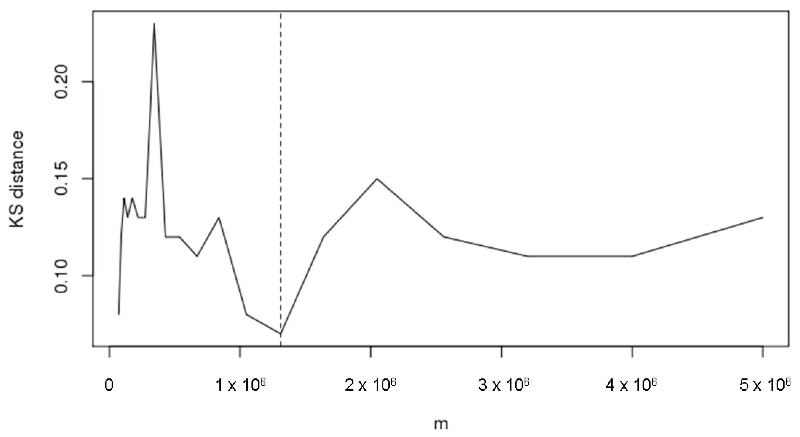
Bickel and Sakov (2008) propose to use the Kolmogorov-Smirnov distance, i.e., $\rho (F,G)={\sup }_x|F\left(x\right)-G\left(x\right)|$, for measuring the distance. The adaptive rule described above has been applied on our example to choose m (where n is equal to 5 millions), with parameter $q=0.8$ to define $m_j$. Figure 1 shows the Kolmogorov-Smirnov distances, calculated for each $m_j$ over the grid of values in 1–5 millions as in (19) with $q=0.8$, to select the value of $\widehat{m}$ which minimizes the discrepancies among bootstrap distributions. The Kolmogorov-Smirnov distance has been minimized for $\widehat{m}$ = 1,310,721.

We get the $99.9\%$ quantile estimate

$$Va{R}^{m-boot}\left(0.999\right)=47.8173\times {10}^6$$

(21)

from the sample average of the $B=100$ estimated $99.9\%$ quantiles calculated using the Monte Carlo samples of size $\widehat{m}$ = 1,310,721. We employ the empirical $0.05$ and $0.95$ quantiles of the $B=100$ realizations of the $99.9\%$ quantiles calculated using the Monte Carlo samples to obtain the CI

$$[L^{m-boot};R^{m-boot}]=[46.9388\times {10}^6;48.9690\times {10}^6].$$

(22)

As before, we evaluate the error

$$E^{m-boot}=(R^{m-boot}-L^{m-boot})=2.0302\times {10}^6$$

(23)

and the relative error

$$R{E}^{m-boot}=(R^{m-boot}-L^{m-boot})/Va{R}^{m-boot}\left(0.999\right)=0.042457=4.2457\%.$$

(24)

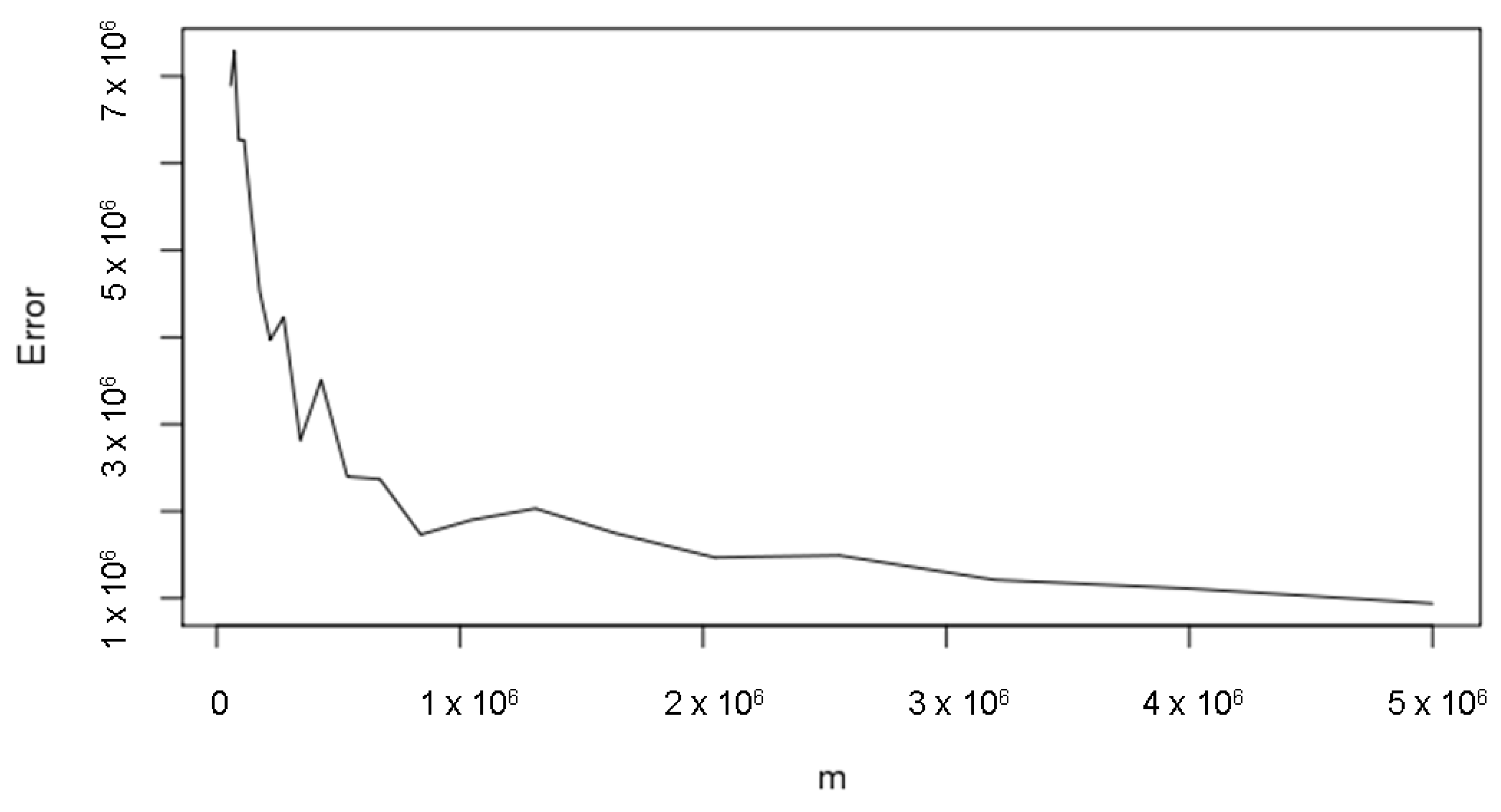
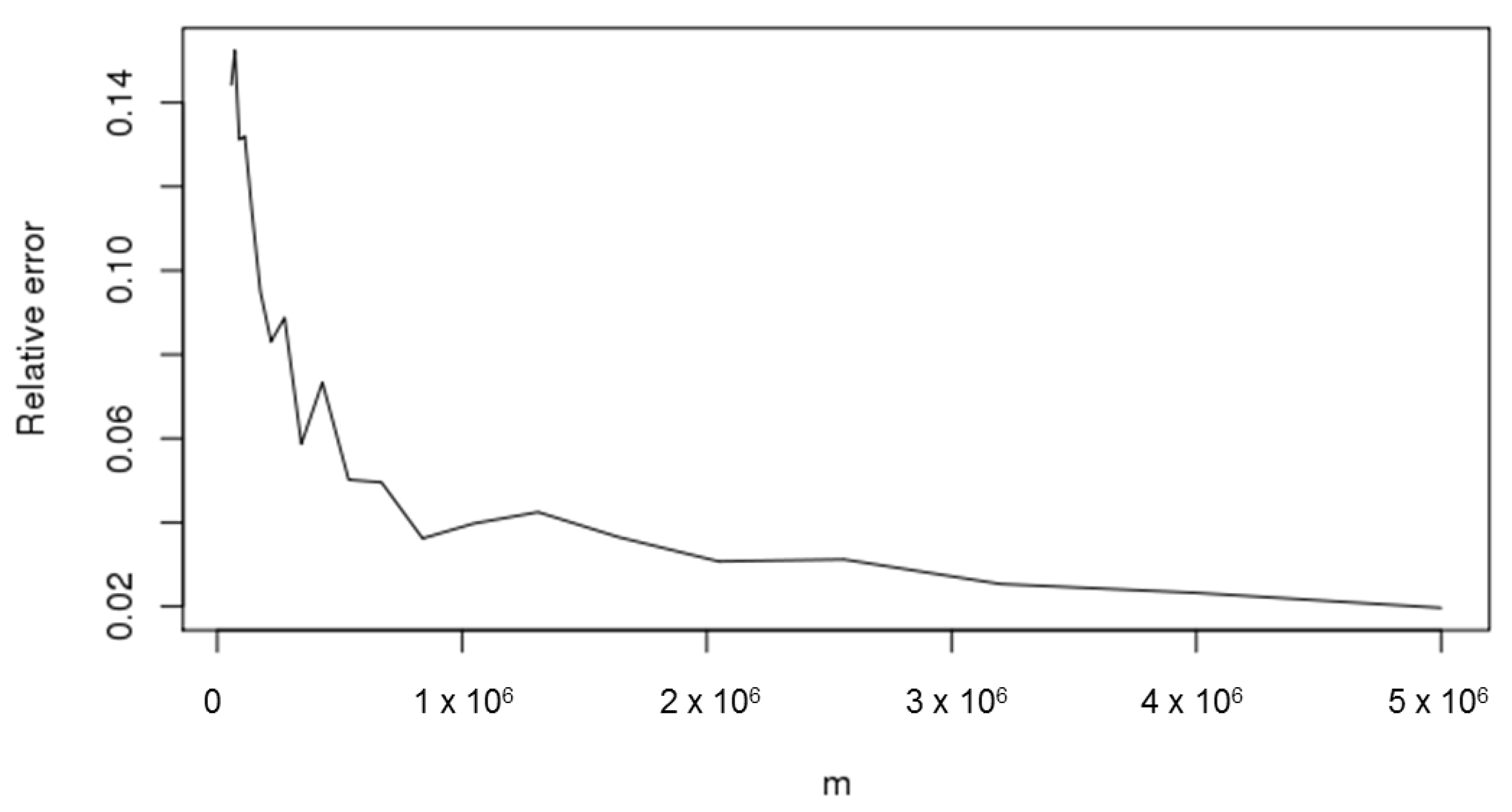
We note that by applying the m-out-of-n-bootstrap with $\widehat{m}$ = 1,310,721, the error and the relative error are slightly higher than the double of the same values calculated using the n-bootstrap. We can observe that this result is consistent with the fact that the Monte Carlo accuracy increases (decreases) proportionally to the square root of the number of steps: since the ratio between n = 5,000,000 and $\widehat{m}$ = 1,310,721 is equal to around 3.8, we can expect that the relative error increases by approximately $\sqrt{3.8}=1.95$, which is actually close to the observed result. To see the impact of the selection of $\widehat{m}$, Figure 2 and Figure 3 depict the errors and the relative errors of the CIs calculated on the grid of values of m as in (19).

We observe that the errors decrease as the value of m increases, which is consistent with the aforementioned square root rule for the Monte Carlo accuracy.

4.4. The Monte Carlo Repetition Method

In this section, we compare the previous results with those we shall next obtain using the Monte Carlo repetition method. We first note that repeating the Monte Carlo method several times, without fixing the initial seed of each repetition, provides a realistic probability distribution of the possible results that we can obtain using this numerical procedure. Please note that it is fundamental to initialize the seed only for the first repetition since, as reminded in Section 2, the seed defines the entire sequence of the generated random numbers. In fact, if we initialize the same seed for each Monte Carlo repetition, we will alway obtain the same results leading to a degenerate probability distribution. Although the Monte Carlo repetition method can be intuitively considered as the most accurate to estimate the Monte Carlo error (if the number of repetitions is sufficient), it cannot be extensively used because it is the most computationally intensive. Therefore, to compare the Monte Carlo repetition method with previous results, we simulate the distribution of the quantile by repeating 100 times the Monte Carlo method. We get the $99.9\%$ quantile estimate

$$Va{R}^{MC100}\left(0.999\right)=47.4246\times {10}^6$$

(25)

from the sample average of the 100 estimated $99.9\%$ quantiles, calculated on the 100 Monte Carlo samples. We employ the empirical $0.05$ and $0.95$ quantiles of the $99.9\%$ quantiles calculated from the 100 Monte Carlo samples to obtain the CI

$$[L^{MC100};R^{MC100}]=[47.0261\times {10}^6;47.8522\times {10}^6].$$

(26)

As before, we evaluate the error

$$E^{MC100}=(R^{MC100}-L^{MC100})=0.8261\times {10}^6$$

(27)

and the relative error

$$R{E}^{MC100}=(R^{MC100}-L^{MC100})/Va{R}^{MC100}\left(0.999\right)=0.017420=1.7420\%.$$

(28)

We note that the current method provides slightly lower errors than the previous two methods.

To see how the number of Monte Carlo repetitions affects the results, we have reapplied the current method by repeating 1000 times the Monte Carlo method. We obtain the following results:

$$Va{R}^{MC1000}\left(0.999\right)=47.4345\times {10}^6;$$

(29)

$$[L^{MC1000};R^{MC1000}]=[47.0207\times {10}^6;47.8503\times {10}^6];$$

(30)

$$E^{MC1000}=(R^{MC1000}-L^{MC1000})=0.8297\times {10}^6;$$

(31)

$$R{E}^{MC1000}=(R^{MC1000}-L^{MC1000})/Va{R}^{MC1000}\left(0.999\right)=0.017491=1.7491\%.$$

(32)

Please note that even though we have increased the number of repetitions from 100 to 1000, the error results basically remain the same.

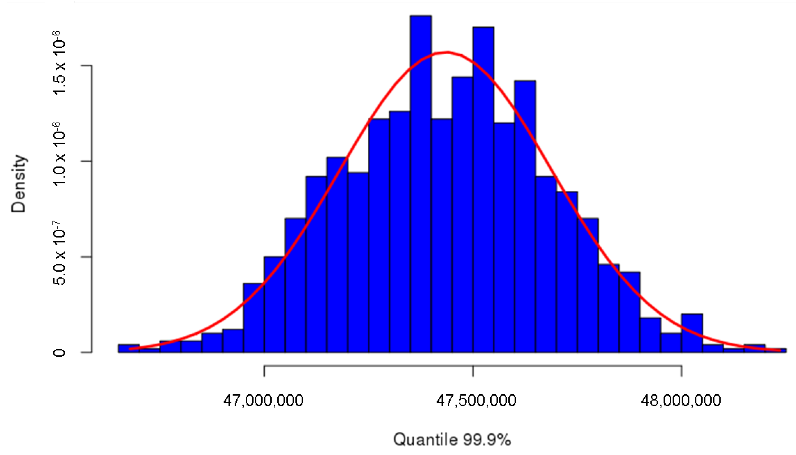
To obtain a further confirmation of the sufficiency of 1000 repetitions, we check the normality of the distribution of the 99.9% quantile. First of all, we estimate the parameter of the normal distribution from the sample average $\mu =47.4345\times {10}^6$ and the sample standard deviation $\sigma =0.2540\times {10}^6$. Figure 4 depicts the histogram of the simulated 99.9% quantiles derived from the 1000 samples. It is apparent that it follows the normal distribution.

As an additional check for the normality assumption, we apply the Shapiro-Wilk test using the R function shapiro.test, see R Core Team (2016). The p-value of the test is 0.4642, implying that the normality distribution cannot be rejected due to being considerably higher than 0.05.

4.5. Constrained Optimization Methods

In this section, we introduce two alternative methods for estimating the Monte Carlo error. In fact, we have not seen these methods introduced earlier in the literature.

Adopting the earlier notation introduced and setting $k=\left[np\right]$, it is natural to base the interval estimation for the $99.9\%$ quantile on the order statistic $X_{k:n}=F_n^{-1}\left(p\right)$. We look for the shortest interval $[a,b]\subset \mathbb{R}$ such that

$$\mathbb{P}\{a<X_{k:n}\le b\}=0.9.$$

(33)

Let $\alpha ,\beta \in [0,1]$ be such that and $F^{-1}\left(\alpha \right)=a$ and $F^{-1}\left(\beta \right)=b$, and let

$$\mathbb{P}\{a<X_{k:n}\le b\}=\mathbb{P}\{F^{-1}\left(\alpha \right)<X_{k:n}\le F^{-1}\left(\beta \right)\}=0.9.$$

(34)

We know that $\mathbb{P}\{X_{k:n}\le x\}={\sum }_{j=k}^n\left(\genfrac{}{}{0pt}{}{n}{j}\right)F^j\left(x\right){(1-F\left(x\right))}^{n-j}$. Therefore

$$\mathbb{P}\{F^{-1}\left(\alpha \right)<X_{k:n}\le F^{-1}\left(\beta \right)\}=\sum _{j=k}^n\left(\genfrac{}{}{0pt}{}{n}{j}\right){\beta }^j{(1-\beta )}^{n-j}-\sum _{j=k}^n\left(\genfrac{}{}{0pt}{}{n}{j}\right){\alpha }^j{(1-\alpha )}^{n-j}$$

and the CI for $F^{-1}\left(p\right)$ is obtained by searching for $\alpha$ and $\beta$ such that

• ${\sum }_{j=k}^n\left(\genfrac{}{}{0pt}{}{n}{j}\right){\beta }^j{(1-\beta )}^{n-j}-{\sum }_{j=k}^n\left(\genfrac{}{}{0pt}{}{n}{j}\right){\alpha }^j{(1-\alpha )}^{n-j}=0.9$, and
• $(\beta -\alpha )$ is minimal.

This constrained optimization problem can be solved numerically by considering a grid of $\alpha$ and $\beta$ values close to p.

Equivalently, we can restate our research question into the search of $\alpha$ and $\beta$ such that

• $\mathbb{P}\{\alpha <U_{k:n}\le \beta \}=0.9$, and
• $(\beta -\alpha )$ is minimal,

where $U_{k:n}=F\left(X_{k:n}\right)$ is a uniform r.v. on [0,1]. Here we have used the fact that if X is a continuous random variable with cdf F, then the random variable $U=F\left(X\right)$ has a uniform distribution on [0,1]. Therefore $\alpha$ and $\beta$ can be obtained by repeated draws from uniform random variables on [0,1].

Coming back to the CI for $VaR$, we have

$$\mathbb{P}\{F^{-1}\left(\alpha \right)<F_n^{-1}\left(p\right)\le F^{-1}\left(\beta \right)\}=0.9,$$

that is

$$\mathbb{P}\{F_n^{-1}\left(p\right)\le F^{-1}\left(\beta \right)\}-\mathbb{P}\{F_n^{-1}\left(p\right)\le F^{-1}\left(\alpha \right)\}=0.9.$$

(35)

Note the equations

$$\mathbb{P}\{F_n^{-1}\left(p\right)\le F^{-1}\left(\beta \right)\}=\mathbb{P}\left\{\frac{F^{-1}\left(p\right)}{F^{-1}\left(\beta \right)}{F}_n^{-1}\left(p\right)\le F^{-1}\left(p\right)\right\}$$

and

$$\mathbb{P}\{F_n^{-1}\left(p\right)\le F^{-1}\left(\alpha \right)\}=\mathbb{P}\left\{F_n^{-1}\left(p\right)\frac{F^{-1}\left(p\right)}{F^{-1}\left(\alpha \right)}\le F^{-1}\left(p\right)\right\}.$$

Consequently, Equation (35) becomes

$$\mathbb{P}\left\{\frac{F^{-1}\left(p\right)}{F^{-1}\left(\beta \right)}{F}_n^{-1}\left(p\right)\le F^{-1}\left(p\right)\le \frac{F^{-1}\left(p\right)}{F^{-1}\left(\alpha \right)}{F}_n^{-1}\left(p\right)\right\}=0.9$$

and implies the following CI

$$[L;R]=\left[\frac{{\left(F_n^{-1}\left(p\right)\right)}^2}{F_n^{-1}\left(\beta \right)};\frac{{\left(F_n^{-1}\left(p\right)\right)}^2}{F_n^{-1}\left(\alpha \right)}\right]$$

where $\beta$ and $\alpha$ are functions of n and p obtained using any of the two methods presented earlier.

Next are the results obtained using the first constrained optimization method:

$$Va{R}^{O1}\left(0.999\right)=47.8037\times {10}^6,$$

(36)

$$[L^{O1};R^{O1}]=[47.3399\times {10}^6;48.2386\times {10}^6],$$

(37)

$$E^{O1}=(R^{O1}-L^{O1})=0.8987\times {10}^6,$$

(38)

$$R{E}^{O1}=(R^{O1}-L^{O1})/Va{R}^{O1}\left(0.999\right)=0.018799=1.8799\%.$$

(39)

The second constrained optimization method yields the following results:

$$Va{R}^{O2}\left(0.999\right)=47.8037\times {10}^6,$$

(40)

$$[L^{O2};R^{O2}]=[47.4584\times {10}^6;49.0432\times {10}^6],$$

(41)

$$E^{O2}=(R^{O2}-L^{O2})=1.5848\times {10}^6,$$

(42)

$$R{E}^{O2}=(R^{O2}-L^{O2})/Va{R}^{O2}\left(0.999\right)=0.033153=3.3153\%.$$

(43)

We observe that the second method provides a higher relative error, probably due to the less accurate evaluation of $\alpha$, obtained by redrawing from the uniform distribution on [0,1]. In fact, while in the first constrained optimization method we used a grid of 10,000 points close to p, in the second one we drew 10,000 values from the uniform distribution on [0,1]. These configurations were used to have a comparable computational effort between the two methods. The obtained results suggest that the second constrained optimization method would require a higher computational effort to reach a relative error comparable to the first one.

4.6. Comparison among the Described Methods

All the results that we have obtained using the methods discussed in this paper are summarized in

Table 1. Estimated Monte Carlo errors (values in millions of Euro).

Method	VaR(0.999)	L	R	E	$\mathit{RE}$
Binomial	47.8037	47.3667	48.2897	0.9231	1.9310%
n-Bootstrap (100 samples)	47.7977	47.2914	48.2306	0.9392	1.9649%
m-out-of-n-Bootstrap (100 samples)	47.8173	46.9388	48.9690	2.0302	4.2457%
MC repetitions (100 samples)	47.4246	47.0261	47.8522	0.8261	1.7420%
MC repetitions (1000 samples)	47.4345	47.0207	47.8503	0.8297	1.7491%
Constrained optimization I	47.8037	47.3399	48.2386	0.8987	1.8799%
Constrained optimization II	47.8037	47.4584	49.0432	1.5848	3.3153%

. We applied different methodologies for constructing CI’s for the VaR to realistic data samples, mimicking annual loss distributions and obtained via the Monte Carlo method with 5 million steps based on the lognormal (9,2) severity distribution and the Poisson (100) frequency distribution. First of all, we see from Table 1 that all the approaches (apart from the m-out-of-n-bootstrap and the constrained optimization II, for the above mentioned reasons) are consistent with each other, and the method based on Monte Carlo repetitions is slightly less conservative than the other methods. On the other hand, the binomial method allows obtaining consistent results with the great advantage of requiring much less computational effort. In fact, the binomial method allows constructing the CI for the VaR using closed forms and, on the contrary to other methods, does not require to perform further simulations. Applying the Monte Carlo repetition method, in both cases considering 100 and 1000 samples, and the binomial, n-bootstrap and constrained optimization I methods, we obtain a relative error not higher than 2%. Therefore, whenever we fix the tolerance threshold for the relative error equal to 2%, we can conclude that 5 million steps are sufficient to mitigate sampling errors, as prescribed in EU Regulation 2018/959. For tolerance thresholds lower than 2%, we presumably have to increase the number of Monte Carlo steps or, alternatively, we have to adopt more sophisticated approaches, such as the variance reduction techniques or the Quasi-Monte Carlo methods.

5. Conclusions and Further Work

Motivated by the recently published EU Regulatory Technical Standards on AMA models, we have analyzed and compared six methods to estimate the Monte Carlo error when estimating VaR in operational risk measurement. The purpose is to assess the capital charge for the financial institution, usually defined through the VaR measure as the 99.9% quantile of the annual loss distribution with the holding period of one year. Presently, financial analysts and regulators are more and more focused on how to mitigate sampling errors, and this concerns the assessment of CI’s for the Value-at-Risk along the lines of EU Regulation 959/2018. In this paper we have aimed at offering to practitioners an easy-to-follow rule of thumb for choosing approaches to evaluate such CI’s and, if needed, for tuning them in terms of the number of required Monte Carlo replications. In particular, we started with the more straightforward method based on the binomial distribution, and we compared it with other methods such as the n-bootstrap, the m-out-of-n-bootstrap, the Monte Carlo repetition method, and two other techniques based on constrained optimization. All the methods have been applied to realistic simulated data. Our results show that the method based on Monte Carlo repetitions is slightly less conservative than the other methods. Furthermore, we have seen that the m-out-of-n-bootstrap and the second method based on constrained optimization give less precise results, in terms of relative error. The binomial method, which requires a much lower computational effort, seems to be particularly useful for the purpose, due to its precision. In fact, the binomial method is just slightly more conservative than the Monte Carlo repetition method, which can be intuitively considered as the most accurate for estimating the Monte Carlo error. Moreover, it is worth mentioning that the more sophisticated Monte Carlo methods, such as the variance reduction techniques and Quasi-Monte Carlo methods, offer several promising technical avenues for implementing the operational risk capital requirement estimation methods that we discussed. They can be subjects for future research.

References

- Bazzarello, Davide, Bert Crielaard, Fabio Piacenza, and Aldo Soprano. 2006. Modeling insurance mitigation on operational risk capital. Journal of Operational Risk 1: 57–65. [Google Scholar] [CrossRef]
- Bickel, Peter J., and Anat Sakov. 2008. On the choice of m in the m out of n bootstrap and confidence bounds for extrema. Statistica Sinica 18: 967–85. [Google Scholar]
- Bickel, Peter J., Friedrich Götze, and Willem R. van Zwet. 1997. Resampling fewer than n observations: Gains, losses, and remedies for losses. Statistica Sinica 7: 1–31. [Google Scholar]
- Böcker, Klaus, and Claudia Klüppelberg. 2005. Operational VaR: A closed-form approximation. Risk Magazine 18: 90–93. [Google Scholar]
- Böcker, Klaus, and Jacob Sprittulla. 2006. Operational VaR: Meaningful means. Risk Magazine 19: 96–98. [Google Scholar]
- Bolancé, Catalina, Montserrat Guillén, Jim Gustafsson, and Jens Perch Nielsen. 2012. Quantitative Operational Risk Models. Abingdon: CRC Press, Taylor & Francis Group. [Google Scholar]
- Boos, Dennis D. 1984. Using extreme value theory to estimate large percentiles. Technometrics 26: 33–39. [Google Scholar] [CrossRef]
- Boyle, Phelim P. 1977. Options: A monte carlo approach. Journal of Financial Economics 4: 323–38. [Google Scholar] [CrossRef]
- Cavallo, Alexander, Benjamin Rosenthal, Xiao Wang, and Jun Yan. 2012. Treatment of the data collection threshold in operational risk: A case study with the lognormal distribution. Journal of Operational Risk 7: 3–38. [Google Scholar] [CrossRef]
- Chen, E. Jack, and W. David Kelton. 2001. Quantile and histogram estimation. Paper Presented at the 2001 Winter Simulation Conference, Arlington, VA, USA, December 9–12. [Google Scholar] [CrossRef]
- Chernobai, Anna, Svetlozar T. Rachev, and Frank J. Fabozzi. 2005. Composite goodness-of-fit tests for left-truncated loss samples. Handbook of Financial Econometrics and Statistics, 575–96. [Google Scholar] [CrossRef]
- Colombo, Andrea, Alessandro Lazzarini, and Silvia Mongelluzzo. 2015. A weighted likelihood estimator for operational risk data: Improving the accuracy of capital estimates by robustifying maximum likelihood estimates. Journal of Operational Risk 10: 47–108. [Google Scholar] [CrossRef]
- Cope, Eric W., Giulio Mignola, G. Antonini, and R. Ugoccioni. 2009. Challenges in Measuring Operational Risk From Loss Data. Technical Report. Torino: IBM Zurich Research Lab, Intesa Sanpaolo SpA. [Google Scholar]
- Cortés, Lina M., Andrés Mora-Valencia, and Javier Perote. 2017. Measuring firm size distribution with semi-nonparametric densities. Physica A 485: 35–47. [Google Scholar] [CrossRef]
- Dalla Valle, Luciana, and Paolo Giudici. 2008. A bayesian approach to estimate the marginal loss distributions in operational risk management. Computational Statistics & Data Analysis 52: 3107–27. [Google Scholar]
- Danesi, Ivan Luciano, and UniCredit Business Integrated Solutions. 2015. Robust Estimators for Operational Risk: A Computationally Efficient Approach. Technical Report. Working Paper Series No. 63; Milano: UniCredit & Universities. [Google Scholar]
- Danesi, Ivan Luciano, Fabio Piacenza, Erlis Ruli, and Laura Ventura. 2016. Optimal B-robust posterior distributions for operational risk. Journal of Operational Risk 11: 1–20. [Google Scholar] [CrossRef]
- Danielsson, Jon, and Casper G. De Vries. 1996. Tail index and quantile estimation with very high frequency data. Journal of Empirical Finance 4: 241–57. [Google Scholar] [CrossRef]
- Di Clemente, Annalisa, and Claudio Romano. 2004. A copula-extreme value theory approach for modelling operational risk. In Operational Risk Modelling and Analysis: Theory and Practice. Edited by M. Cruz. London: Risk Books, vol. 9, pp. 189–208. [Google Scholar]
- Efron, Bradley. 1979. Bootstrap methods: Another look at the jackknife. The Annals of Statistics 7: 1–26. [Google Scholar] [CrossRef]
- Efron, Bradley. 1982. The Jackknife, the Bootstrap and Other Resampling Plans. Number 38 in Regional Conference Series in Applied Mathematics; Philadelphia: Society for Industrial and Applied Mathematics. [Google Scholar]
- Embrechts, Paul, and Marco Frei. 2009. Panjer recursion versus fft for compound distributions. Mathematical Methods of Operations Research 69: 497–508. [Google Scholar] [CrossRef]
- European Parliament and Council of the European Union. 2013. Capital Requirement Regulations. Technical Report, European Union. Available online: https://eur-lex.europa.eu/eli/reg/2013/575/oj (accessed on 26 June 2013).
- European Parliament and Council of the European Union. 2018. Regulatory Technical Standards of the Specification of the Assessment Methodology Under Which Competent Authorities Permit Institutions to Use AMA for Operational Risk. Technical Report, European Union. Available online: https://eur-lex.europa.eu/legal-content/GA/TXT/?uri=CELEX:32018R0959 (accessed on 14 March 2008).
- Figini, Silvia, Lijun Gao, and Paolo Giudici. 2014. Bayesian operational risk models. Journal of Operational Risk 10: 45–60. [Google Scholar] [CrossRef]
- Frachot, Antoine, Pierre Georges, and Thierry Roncalli. 2001. Loss Distribution Approach for Operational Risk. Technical Report. Lyonnais. Available online: http://www.thierry-roncalli.com/download/lda-practice.pdf (accessed on 7 May 2003).
- Frachot, Antoine, Olivier Moudoulaud, and Thierry Roncalli. 2007. Loss distribution approach in practice. In The Basel Handbook: A Guide for Financial Practitioners. Edited by Michael Ong and Jorg Hashagen. London: Risk Books, pp. 527–55. [Google Scholar]
- Gomes, M. Ivette, and Dinis Pestana. 2007. A sturdy reduced-bias extreme quantile (var) estimator. Journal of the American Statistical Association 102: 280–92. [Google Scholar] [CrossRef]
- Gribkova, Nadezhda V., and Roelof Helmers. 2011. On the consistency of the m < < n bootstrap approximation for a trimmed mean. Theory of Probability and Its Applications 55: 42–53. [Google Scholar]
- Guharay, Sabyasachi, K. C. Chang, and Jie Xu. 2016. Robust estimation of value-at-risk through correlated frequency and severity model. Paper presented at 19th International Conference on Information Fusion, Heidelberg, Germany, July 5–8. [Google Scholar]
- Kalos, Malvin H., and Paula A. Whitlock. 2008. Monte Carlo Methods. New York: Wiley. [Google Scholar]
- Kleiber, Christian, and Samuel Kotz. 2003. Statistical Size Distributions in Economics and Actuarial Sciences. New York: Wiley. [Google Scholar]
- Kleijnen, Jack P. C., Ad A. N. Ridder, and Reuven Y. Rubinstein. 2010. Variance reduction techniques in monte carlo methods. Encyclopedia of Operations Research and Management Science, 1598–610. [Google Scholar] [CrossRef]
- Klugman, Stuart A., Harry H. Panjer, and Gordon E. Willmot. 2012. Loss Models: From Data to Decisions, 4th ed. New York: Wiley. [Google Scholar]
- Lambrigger, Dominik D., Pavel V. Shevchenko, and Mario V. Wüthrich. 2007. The quantification of operational risk using internal data, relevant external data and expert opinion. Journal of Operational Risk 2: 3–27. [Google Scholar] [CrossRef]
- Larsen, Paul. 2016. Operational risk models and asymptotic normality of maximum likelihood estimation. Journal of Operational Risk 11: 55–78. [Google Scholar] [CrossRef]
- Larsen, Paul. 2019. Maximum likelihood estimation error and operational value-at-risk stability. Journal of Operational Risk 14: 1–23. [Google Scholar] [CrossRef]
- Lavaud, Sophie, and Vincent Lehérissé. 2014. Goodness-of-fit tests and selection methods for operational risk. Journal of Operational Risk 9: 21–50. [Google Scholar] [CrossRef]
- L’ecuyer, Pierre. 1999. Good parameters and implementations for combined multiple recursive random number generators. Operations Research 47: 159–64. [Google Scholar] [CrossRef]
- Luo, Xiaolin, Pavel V. Shevchenko, and John B. Donnelly. 2007. Addressing the impact of data truncation and parameter uncertainty on operational risk estimates. Journal of Operational Risk 2: 3–26. [Google Scholar] [CrossRef]
- Makarov, Mikhail. 2006. Extreme value theory and high quantile convergence. Journal of Operational Risk 1: 51–57. [Google Scholar] [CrossRef]
- Matsumoto, Makoto, and Takuji Nishimura. 1998. Mersenne twister: A 623-dimensionally equidistributed uniform pseudo-random number generator. ACM Transactions on Modeling and Computer Simulation 8: 3–30. [Google Scholar] [CrossRef]
- Metropolis, Nicholas, Arianna W. Rosenbluth, Marshall N. Rosenbluth, Augusta H. Teller, and Edward Teller. 1953. Equations of state calculations by fast computing machines. Journal of Chemical Physics 21: 1087–91. [Google Scholar] [CrossRef]
- Mignola, Gulio, and Roberto Ugoccioni. 2005. Tests of extreme value theory. Operational Risk 6: 32–35. [Google Scholar]
- Mignola, Gulio, and Roberto Ugoccioni. 2006. Sources of uncertainty in modeling operational risk losses. Journal of Operational Risk 1: 33–50. [Google Scholar] [CrossRef]
- Owen, Art B. 2013. Monte Carlo Theory, Methods and Examples. Stanford: Department of Statistics, Stanford University. [Google Scholar]
- Panjer, Harry H. 2006. Operational Risk: Modeling Analytics. New York: Wiley. [Google Scholar]
- Peng, Liang, and Yongcheng Qi. 2006. Confidence regions for high quantiles of a heavy tailed distribution. Ann. Statist. 34: 1964–86. [Google Scholar] [CrossRef]
- R Core Team. 2016. R: A Language and Environment for Statistical Computing. Vienna: R Foundation for Statistical Computing. [Google Scholar]
- Richtmyer, Robert D. 1952. The Evaluation of Definite Integrals, and a Quasi-Monte Carlo Method Based on the Properties of Algebraic Numbers. Technical Report, LA-1342. Los Angeles: University of California. [Google Scholar]
- Sakov, Anat. 1998. Using the m out n Bootstrap in the Hypothesis Testing. Berkeley: University of California. [Google Scholar]
- Shevchenko, Pavel V. 2011. Modelling Operational Risk Using Bayesian Inference. New York: Springer. [Google Scholar]
- Shevchenko, Pavel V., and Mario V. Wuthrich. 2006. The structural modelling of operational risk via bayesian inference: Combining loss data with expert opinions. Journal of Operational Risk 1: 3–26. [Google Scholar] [CrossRef]
- Student. 1908. The probable error of a mean. Biometrika 6: 1–25. [Google Scholar] [CrossRef]
Figure 1.
Choice of the optimal m in terms of KS distance from bootstrap distributions (n = 5,000,000).
Figure 2.
Error for different m values.
Figure 3.
Relative error for different m values.
Figure 4.
Histogram of 99.9% quantiles derived from 1000 Monte Carlo repetitions, compared with the estimated normal distribution.