Joshi’s Split Tree for Option Pricing


1
Department of Mathematics, American University of Sharjah, P.O. Box 26666, Sharjah, UAE
2
Department of Mathematics, University of Kaiserslautern, 67653 Kaiserslautern, Germany
*
Author to whom correspondence should be addressed.
Risks 2020, 8(3), 81; https://0-doi-org.brum.beds.ac.uk/10.3390/risks8030081
Submission received: 6 July 2020
/
Revised: 22 July 2020
/
Accepted: 24 July 2020
/
Published: 1 August 2020
(This article belongs to the Special Issue Computational Finance and Risk Analysis in Insurance)
Abstract
:In a thorough study of binomial trees, Joshi introduced the split tree as a two-phase binomial tree designed to minimize oscillations, and demonstrated empirically its outstanding performance when applied to pricing American put options. Here we introduce a “flexible” version of Joshi’s tree, and develop the corresponding convergence theory in the European case: we find a closed form formula for the coefficients of and in the expansion of the error. Then we define several optimized versions of the tree, and find closed form formulae for the parameters of these optimal variants. In a numerical study, we found that in the American case, an optimized variant of the tree significantly improved the performance of Joshi’s original split tree.
1. Motivation and Outline
There is a vast collection of literature describing numerical methods for evaluating options. Among the most popular ones is the binomial tree method which is broadly used because of its simplicity and flexibility. In most binomial models, the price of a call/put option is connected to the price of the same call/put option in the Black–Scholes model via an equation of the form
where is bounded but usually not constant, as it depends on n. When is constant, one can use Richardson extrapolation to achieve convergence at a speed of order . For European options, models have been found Joshi (2009b); Leduc (2016a) for which the error has the form
for an arbitrary value of . Obviously, there is a well-known closed form formula for the price of European put/call options in the Black–Scholes model. However, this is not the case for the American put. Yet techniques developed for path-independent European options proved to extend to the study of path-dependent options—for instance, in Bock and Korn (2016); Carbone (2004); Grosse-Erdmann and Heuwelyckx (2016); Heuwelyckx (2014); Leduc and Palmer (2019); Lin and Palmer (2013). Note that the behavior of American options is also connected to the behavior of European options: the American put can be expressed as the sum of a European put and an integral of digital options Carr, Jarrow and Myneni (1992).
Many binomial trees have been suggested in the literature for computing option prices—among others, Chance (2008); Chang and Palmer (2007); Chriss (1996); Cox, Ross and Rubinstein (1979); Diener and Diener (2004); Jarrow and Rudd (1983); Jarrow and Turnbull (2000); Joshi (2009a, 2010); Korn and Müller (2013); Lamberton (1998); Leduc (2016b); Leisen and Reimer (1996); Tian (1993, 1999); Trigeorgis (1991); Van Den Berg and Koudjeti (2000); Walsh (2003); Wilmott (1998). In addition to the intellectual curiosity of understanding how tree models converge to their limits (which is part of the important study of random sums of random variables), the interest in tree methods for pricing security derivatives is motivated by those cases where no simple closed form formula exists. This is the case for American options, for which explicit values for the coefficients in the expansion of the error
are unknown, and finding them is a challenging and interesting problem. Even the speed of convergence of binomial trees to its Black–Scholes limit remains a long lasting and difficult problem Lamberton (1998, 2002, 2018). Thus far, only convergence has been established Amin and Khanna (1994); Jiang and Dai (2004); Lamberton (1993). However, Joshi (2009b) pointed out that trading houses need to efficiently price thousands of American options, and that understanding which tree is the best at doing so is an important problem. Because of the lack of theoretical results, such questions and a lot of the insight about the behavior of the convergence of tree methods for American put options have been assessed through empirical studies, such as Broadie and Detemple (1996); Chan et al. (2009); Chen and Joshi (2012); Hull and White (1988); Joshi (2009b, 2012); Staunton (2005); Tian (1999). Joshi (2009b) studied a broad collection of trees for pricing American options, and found that the most effective ones are the one from Tian (1993) and the split tree which was specifically designed by Joshi to minimize the oscillations of the error. However, the convergence theory for the split tree has never been done. The goal of this paper is to describe and generalize the split tree, analyze and optimize its convergence in the European case, and numerically verify that variants of the split tree introduced in this paper significantly improve the convergence of Joshi’s original split tree in the American case.
First we introduce a “flexible” version of Joshi’s original split tree. In Joshi’s original split tree, a drift parameter is used in the binomial model up to a split time , after which the tree becomes a Cox Ross Rubinstein (CRR) tree. Moreover, Joshi sets the split time to be the first time step greater than or equal to half of the maturity, and he sets the drift parameter in such a way that after the split, half the nodes of the tree are located on each side of the strike K. We relax these constraints on and for the flexible split tree, and we only require that the strike be exactly halfway between two nodes in the log-space, in order to maintain smoothness of the convergence. Joshi’s original split tree is illustrated in Figure 1 where, for simplicity, the log-transformed values of the tree are displayed.
Next we analyze the convergence of the split tree in the European case. For self-similar binomial trees (those for which the up and down mechanism is identical at every time step) the coefficients in the expansion of the error (1) can be calculated with great generality using Diener and Diener (2004) or Chang and Palmer (2007). However, the split tree is not self-similar because it is the mixture of two trees: a flexible binomial tree as in Chang and Palmer (2007), and the Cox Ross Rubinstein (CRR) tree. Hence Diener and Diener (2004) or Chang and Palmer (2007) cannot be used to calculate . The calculation of is the first result of this paper. To the best of our knowledge, it is the first time that an explicit error formula has been found for non-self-similar trees.
Then we define optimal versions of the split tree. When fixing all the parameters of a split tree except its split time , we say that a split time is the optimal split time if the magnitude of the coefficient in (1) is minimized when the split time is . When is the optimal split time, we say that the tree is an optimal split tree. First we prove a general result which provides a close form formula for the optimal split time . However, there are many optimal split trees, even when the parameters , K, r, , and T are fixed. We consider optimal split trees under three natural constraints. The first constraint is to have all the nodes in the final layer of the tree centered around the strike K, as in Joshi’s original split tree. Joshi’s arbitrarily fast converging tree for European vanilla options Joshi (2010) is also centered around the strike. This motivates studying the optimal split tree under this natural constraint, and we call it the optimal centered split tree. However, the “centered” constraint sometimes prevents us from getting . This is our motivation for the maximal range optimal split tree, which is the optimal split tree under the constraint that the range of values of the spot for which at the optimal split time is maximized. Now, the maximal range optimal split tree may result in a very small optimal split time and a large drift . If is very small and the number of time steps n is not large, there can be very few time steps prior to the split time, which may result in increased oscillations of the error. This is the motivation for our last optimal split tree. In the optimal split tree near , we seek to choose the drift in such a way that occurs at a split time which is as close as possible to some target .
Finally, we test our split trees in the American case. Our numerical results suggest that one of our optimal split trees is capable of significantly improving the accuracy of the convergence of Joshi’s original split tree for the American put. We explain how this increased accuracy translates in a measure of increased speed. In this measure, our numerical result suggests that one of our optimal split trees could be significantly faster than Joshi’s original tree.
2. The Split Tree
In the setting of put or call options in the Black–Scholes model with spot price , strike K, risk free rate r, volatility , and maturity T, the binomial tree method with n time steps, is equivalent to replacing the Black–Scholes geometric Brownian motion with a process such that at every positive time t which is a multiple , the process jumps from its current position to with probability p, and jumps to with probability . Such trees are called self-similar because the jumping mechanism is identical at every time step.
Binomial trees typically exhibit an oscillatory convergence, and numerous choices of and p have been proposed to smooth and accelerate this convergence. In the Cox Ross Rubinstein (CRR) model Cox, Ross and Rubinstein (1979), the choices are
In the flexible binomial trees, Chang and Palmer (2007); Tian (1999), the values of u, d, and p are given by
where the additional drift parameter may depend on n but must remain bounded.
Let . In the split tree with split time and drift parameter , the process follows a flexible binomial tree with parameter on the interval , and it follows the CRR model thereafter. This means that the values of d and p used to calculate
at time are constant for and . In fact, the split tree uses u, d, and p from (4) for , and it uses (3) for . Seeking good convergence properties, the split tree requires that falls exactly halfway between two nodes in the log-space. Here is any number in the interval . However, given a split time , the actual time at which the values of u and d switch from (4) to (3) can only be a multiple of . When is not a multiple of , we round it to the nearest multiple of . In this manner, we can assume that is a multiple of . Note that the cases where and correspond to no splitting, which is treated in Chang and Palmer (2007). Thus, in order to simplify the exposition, when calculating the coefficient of the error in
we make the assumption that
As for , we can express it in the form
where, for some integer depending on n,
or equivalently
The parameter is actually a practical way of determining because one of the defining properties of the split tree is that falls exactly halfway between two nodes in the log-space and this is guaranteed by (7) and (8). To see this, consider first the special case where n is even, and where with m even. Then an even number of time steps, , is left until maturity T. At time , the tree is centered around
This means that, if at time the total number of up movements is equal to the total number of down movements in the tree, then the value of is . As an even number of time steps is left until maturity, it follows that in the CRR model (and therefore in the split tree) is a terminal node. Hence, in the log space, the terminal nodes of the tree have the form
The cases and give the two neighbors of . Thus, falls exactly halfway between two nodes in the log-space, as claimed. The other cases (n even and m odd, n odd and m odd, and n odd and m even) can be treated in a similar manner. Throughout this paper we make the assumption that satisfies
or equivalently
The simplest way to specify a split tree is via the split time and the implicit parameter ℓ. Here is a formal definition.
Definition 1
(Split tree with parameters and ℓ). Consider a spot price , a strike K, a risk free rate r, a volatility σ, a maturity T, and a number of time steps . Given a split time , and some integer ℓ, define by (8), and define λ by (7). Define also , , and by
Finally, define the time steps , for , by . The split tree with parameter τ and ℓ is the stochastic process which is constant on each interval , such that , and which at every time step , jumps from its current position to with probability , and jumps to with probability .
Definition 2.
We say that a split tree is centered if .
Definition 3.
Joshi’s original split tree is the special case where , and τ is the smallest time step greater than or equal to .
3. Rate of Convergence of the Split Tree
In this section, we provide two expressions for the coefficient of in the expansion in powers of of the error for the split tree value of a call option , against the Black–Scholes price . We also show that the coefficient of is null. Given splitting parameters and , we find an explicit formula for the value of in . Here c is a smooth function of and . In Section 3.1 we provide a generic expression for c, and in Section 3.2 we transform this generic expression into an explicit closed-form formula.
3.1. Generic Expressions for the Coefficients of in the Error
We use the semigroup notation introduced by Leduc in Leduc (2013). Consider any Markov process, for instance, a discrete Markov process , with for some process with independent increments. Consider now , the conditional expectation given that . Then for any non-negative measurable function f, any , and any , the Markov property gives that
Obviously, with
we obtain the discounted expectation semigroup operator. It satisfies
In other words, is the price of an option with maturity t and payoff function f, when .
As always, the strike K, spot price , maturity T, risk free rate r, and volatility are fixed. We denote by the flexible binomial model of Chang and Palmer (2007) with parameter and n time-steps until maturity. Hence is the stochastic process associated with and p given by (4). We denote by its semigroup operator. Note that the CRR model corresponds to a flexible binomial model where . Given a split time and drift parameter , we denote by and the stochastic process and semigroup operator associated with the corresponding split tree. Finally, denotes the semigroup operator associated with the geometric Brownian motion.
To shorten expressions we set
Then
and the price of a call option with maturity T in the split tree model can be written as
Motivated by our extension of the results in Leduc (2013), Theorem A2 in Appendix C, we introduce another abbreviation: given a non negative measurable bounded function h, we write:
where
If h is smooth enough then Theorem A2 says that is the coefficient of in the expansion of the error for an option with payoff h evaluated in the flexible model with parameter when .
Moreover, for every and , we also use the notation
where and are as in Chang and Palmer’s Theorem A1 given in Appendix B; that is,
Note that is the coefficient of in the expansion of the error of a call option in the CRR model when .
Let be the price of a call option in the Black–Scholes model of the option, when the maturity is t, the strike is K, the risk free rate is r, the volatility is , and the spot price is x. The next proposition provides a generic expression that connects the option’s price in the split model to the price in the Black–Scholes model.
Proposition 1.
Consider a European call option with strike K, spot price , maturity T, risk free rate r, and volatility σ. Let the split time , , be bounded away from 0 and T. Moreover, let the drift be bounded and of the form for some of the form (8). Then the price in the Black–Scholes model is related to the price in the split tree model by the equation
where
3.2. Explicit Expressions for the Coefficients of in the Error
It follows from (12) that
The derivatives with respect to the spot price of a call option in the Black–Scholes model are well known, and from there we see that for ,
where is as in Section 3.1, and
The following theorem, proved in Appendix A, provides an explicit closed form formula for the coefficient of in the expansion of the error of a call option evaluated with the split tree.
Theorem 1.
Consider a European call option with strike K, spot price , maturity T, risk free rate r, and volatility σ. Let the split time , , be bounded away from 0 and T. Moreover, let the drift be bounded and of the form for some of the form (8). Then the price in the Black–Scholes model is related to the price in the split tree model by the equation
where
with
Note that when and n is odd, , and regardless of the value of , there is no splitting since the process is CRR throughout. Our error formula therefore coincides with the formula in Chang and Palmer (2007); that is,
Note also that the case does not fall under the assumption of Theorem 1 above. However, when there is actually no splitting and because K is exactly halfway between two nodes; the oscillating term in the formula of Chang and Palmer (2007) vanishes. Simple algebraic manipulations show again that our formula coincides with the formula in Chang and Palmer (2007) (see Theorem A1 in Appendix B); that is
The following provides another expression for which we will use for defining optimal split trees.
Lemma 1.
For , the term can be rewritten as
where
Proof.
This follows from minor algebraic manipulation of (22) after replacing by . ☐
4. Optimal Split Trees
It is natural to optimize the splitting parameters and (or equivalently and ℓ) for performance: we want to minimize the value of in
In fact, we will show in this section that unless is deeply in or out of the money, the splitting parameters can always be chosen in such a way that .
All parameters being fixed except the split time , we say that a split time is the optimal split time if the magnitude of is minimized when is equal to . When the split time is equal to the optimal split time, we say that the tree is an optimal split tree.
In this section we study optimal split trees under three constraints, and under these constraints we find closed form formulae for the optimal split time and the optimal drift parameter .
- For centered trees, where , we find the optimal split time , which minimizes .
- We find and , which maximize the range of values of for which .
- We find and , which minimize the magnitude of under the constraint that is as close as possible to some specific value .
4.1. The Optimal Split Time Given ℓ
Before defining our optimal split trees, we a need a general result which is the topic of this section. Recall that
and that, given a split time ,
Proposition 2
(Minimum of given ℓ). Consider a European call option with strike K, spot price , maturity T, risk free rate r, and volatility σ. Let
Assume that , and consider integers such that is bounded and bounded away from 0. Then the magnitude of the function defined by (25) is minimized when τ takes the value given by
Proof.
We use Lemma 1 to write
If (or equivalently ) then the value of does not depend on . Hence minimizes . Note that . Hence it is clear that for every . Thus, if , then the magnitude of is minimized when . It remains to consider the case where and . Then because and . Moreover, when takes the value . Since and , it is clear that is always strictly positive. It remains to show that . In fact, because is a strictly increasing function of , , and . ☐
Theorem 2
(Optimal splitting time given ℓ). Consider a European call option with strike K, spot price , maturity T, risk free rate r, and volatility σ. Let , , be defined by
Assume that , and consider integers such that is bounded, bounded away from 0, and converges to as . Let , , and be the limits of respectively , , and . When , assume additionally that n is large enough so that . Let given by
Round into , the nearest multiple of in the interval , and consider the value of a call option evaluated in the split tree with parameters ℓ and . If and , then converges to its Black–Scholes limit at a speed of order . Otherwise, the convergence occurs at a speed of order .
Proof.
When , the tree is not a split tree but rather a flexible binomial tree with parameter and the rate of convergence is , as shown in Chang and Palmer (2007).
We just need to consider the case where and . In this case we assume that n is big enough so that is bounded away from 0, and . Note that is bounded. Thus is bounded away from 0. It follows that is also bounded away from 0. From Lemma 1
Because we see that . Note, furthermore, that it is not possible that when , because otherwise
Thus is also bounded away from T. We have shown that is bounded away from 0 and from T.
Finally, the rounding of into its nearest strictly positive time step, , affects the value of
by an amount of order , since is continuously differentiable for and its first derivative, , is bounded. Thus
Theorem 1 then yields that
as wanted. ☐
Remark 1.
When considering optimal split tree with maturity T, the case where can be seen as a degenerate case of the split tree. Trees of this family, introduced by Chang and Palmer (2007), are called flexible trees. We set when the magnitude of the coefficient of in the expansion of the error (5) is not minimized by any split tree but is rather minimized by a flexible tree.
4.2. The Optimal Centered Split Tree
Joshi’s original split tree is a centered split tree because . However, in general, Joshi’s tree is not the optimal centered split tree because it does not minimize the magnitude of the coefficient of in the expansion of the error. This is because is not, in general, the optimal split time. The optimal split time is given by Theorem 2. Note that, obviously, when ,
When noting that , , and converge to where
it is easy to apply Theorem 2 in order to find the optimal split time.
Definition 4
(Optimal centered split tree). Consider a European call option with strike K, spot price , maturity T, risk free rate r, and volatility σ. Let , assume that for every n, and let be as in Theorem 2. The optimal centered split tree is defined to be the split tree with parameters ℓ and .
4.3. The Maximal Range Optimal Split Tree
Recall that if is the price of a call option in a split tree model, and is the corresponding Black–Scholes price, then
In the optimal centered split tree, unless is too deep in or out of money. Otherwise, the value of is minimized. This occurs under the constraint that . Here we want to lift that constraint in order to maximize the range of values of for which can be achieved.
Recall that for split trees
Assume that is bounded, bounded away from zero, and converges to as . Recall and from Theorem 2. Then the optimal time takes the form and when
A glance at (25) reveals that is a polynomial of degree 2 in , and the coefficient of is negative. Alternatively, can also be seen as a polynomial of degree 2 in ,
and again the coefficient of is negative. We want to find the value of (or the corresponding value of ) which maximizes . This maximizes the range of values of for which and are guaranteed.
As a function of , achieves its maximum whenever reaches its maximum. Now is just a polynomial of degree two in ,
Hence it reaches its maximum at
Through the formula (30) and (31), the optimal drift translates into an optimal choice of ℓ given by
or equivalently
We can also write as
where
However, may not be integer, so we round it to the nearest integer . This is essential to preserve the structure of a split tree. Let us write . Obviously . It is easy to verify that
Hence
In this manner we can define the maximal range optimal split tree in a similar manner as we defined the optimal centered split tree.
Definition 5
(Maximal range optimal split tree). Consider a European call option with strike K, spot price , maturity T, risk free rate r, and volatility σ. Let , let be as in (33), let be the nearest integer to , and set for every n. Let be as in Theorem 2. The maximal range optimal split tree is defined to be the split tree with parameters and .
4.4. The Optimal Split Tree Near
Here our goal is to choose as close as possible to in such a way that , or if this cannot be achieved, we want to choose in a way that minimizes .
Let . Then , where
We need to consider three cases. Case (1) . Then it is possible to choose a real value of such that . There are two choices for which are given by
Case (2) and . This implies that . Now if we replace by then . Note that
Note also that the roots of are 0 and . Since , this means that if and only if . Thus . Now there are two possibilities: either or . In the first case the value of that we want is given by
since it gives . In the second case, We understand that for every value of . Hence we want to maximize . This means choosing
Case (3) and . This implies that . In this case, for every x, and thus for every value of and . However, we know from Lemma 1 that regardless of the value of the parameter ℓ, if for every then is maximized when . Hence we select , and we want to maximize . The maximum occurs at
The three cases can be summed up in the following definitions:
and
Using the (30) and (31), with replaced by their approximations we obtain
which can be re-written as
where
In order to preserve the structure of a split tree, is rounded to the nearest integer . From , we obtain as
We define . Obviously . Then
and
The rounded value of appears to be a good estimate of , but nothing guarantees that it is accurate. We need to apply Theorem 2 in order to find from . However, there can be two values of (corresponding to the possible two different values for ). It turns out that we can carefully choose in order to further smooth out the convergence. Note that the choice of exists only when . In this case, Theorem 2 says that
where
Because has oscillations of order , so does . The best choice of D is the one for which these oscillations are minimized. Hence we determine the value of D (and therefore the values of , , , and ) by choosing the value of D for which the magnitude of is minimized. Now
By simplifying, we obtain
where
(Note that the case where is irrelevant since it corresponds to a situation in Theorem 2 where . In this case we can arbitrarily choose the largest value of D.) The following sums up the definition of the optimal split tree near .
Definition 6
(Optimal split tree near ). Consider a European call option with strike K, spot price , maturity T, risk free rate r, and volatility σ. Let , Let be as in (37). In the case where (37) gives two definitions of , choose the one corresponding to the smallest value of (39). Should in (39), choose the largest value of D. Next, let be the nearest integer to , and set for every n. Finally, let be as in Theorem 2. The optimal split tree near τ is defined to be the split tree with parameters and .
5. American Put
5.1. Measuring the Magnitude of the Oscillations of the Error
The split tree was invented by Joshi with the aim Joshi (2009b) of minimizing the oscillations in the convergence of the American put. If is the price of a put option in a tree method and is the price in the Black–Scholes model, then we say that the convergence is smooth if
for some constant . It has been observed—although not proven yet—that models with smooth convergence in the European case also display smooth convergence in the American case. When the convergence is smooth we can use Richardson extrapolation to obtain a value satisfying
where is bounded. Define
The optimal model among a collection of models to be compared is the one for which the quantity is minimized. This is analogous to Korn and Muller’s optimal drift Korn and Müller (2013) which minimizes in (40), where can be written as
and the optimal drift model is the model which minimizes the value of among all those flexible models with smooth convergence. Here is estimated using , with calculated with Joshi’s original split tree. We estimate using
We will compare the value of calculated using Joshi’s original split tree to the the value of calculated with our optimal split trees.
The following lemma provides a connection between the magnitude of the oscillations, , and the computational effort required to estimate the price of an option. We define the computational effort needed to calculate the price of a put option in a binomial tree model with n time-steps to be equal to the number of nodes in the tree, which is .
Lemma 2.
For , let be the value of in model 1 and model 2, respectively. Assume that . Suppose also that, given , the number of time-steps n in model i is chosen in such a way that in the worst case scenario the error is less than ε, that is, in such a way that . Then, asymptotically as , the quotient of the computational effort required with model 1 over the computational effort required in model 2 is . That is, model 2 is times as fast as model 1, or said in other words, model 2 is faster than model 1.
5.2. Numerical Results
We now illustrate numerically our findings for American put options. We consider the optimal centered split tree, the maximal range optimal split tree, and the optimal split tree near . Calculations were perform using the classical Richardson extrapolation; that is, we calculated using
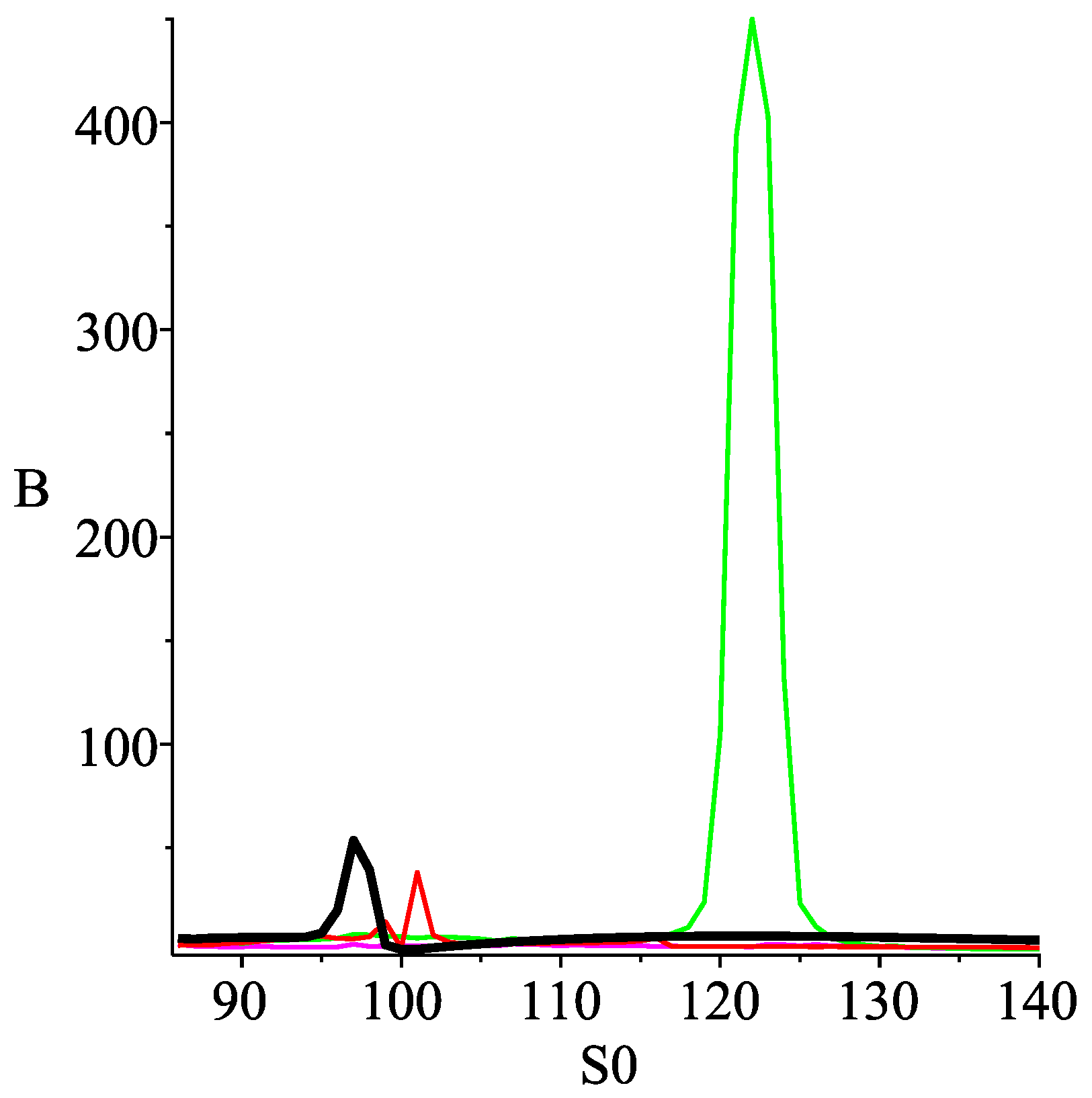
for n even. With , , , , we calculated the values of , estimated by (42), for all integer values of such that , that is, for , where is the price of the option in the Black–Scholes model estimated using Joshi’s original split tree with classical Richardson extrapolation and time steps. The results are shown in Figure 2 and Figure 3.
In Figure 2, we see that the value of for the maximal range optimal split tree spikes at 450 when . The value of in Joshi’s original split tree, traced in a bold font, reaches a maximum of when . Next, the value of peeks at when , for the optimal centered split tree. At the very bottom, the curve for the optimal split tree near is hard to spot. That makes it the best amongst all the models.
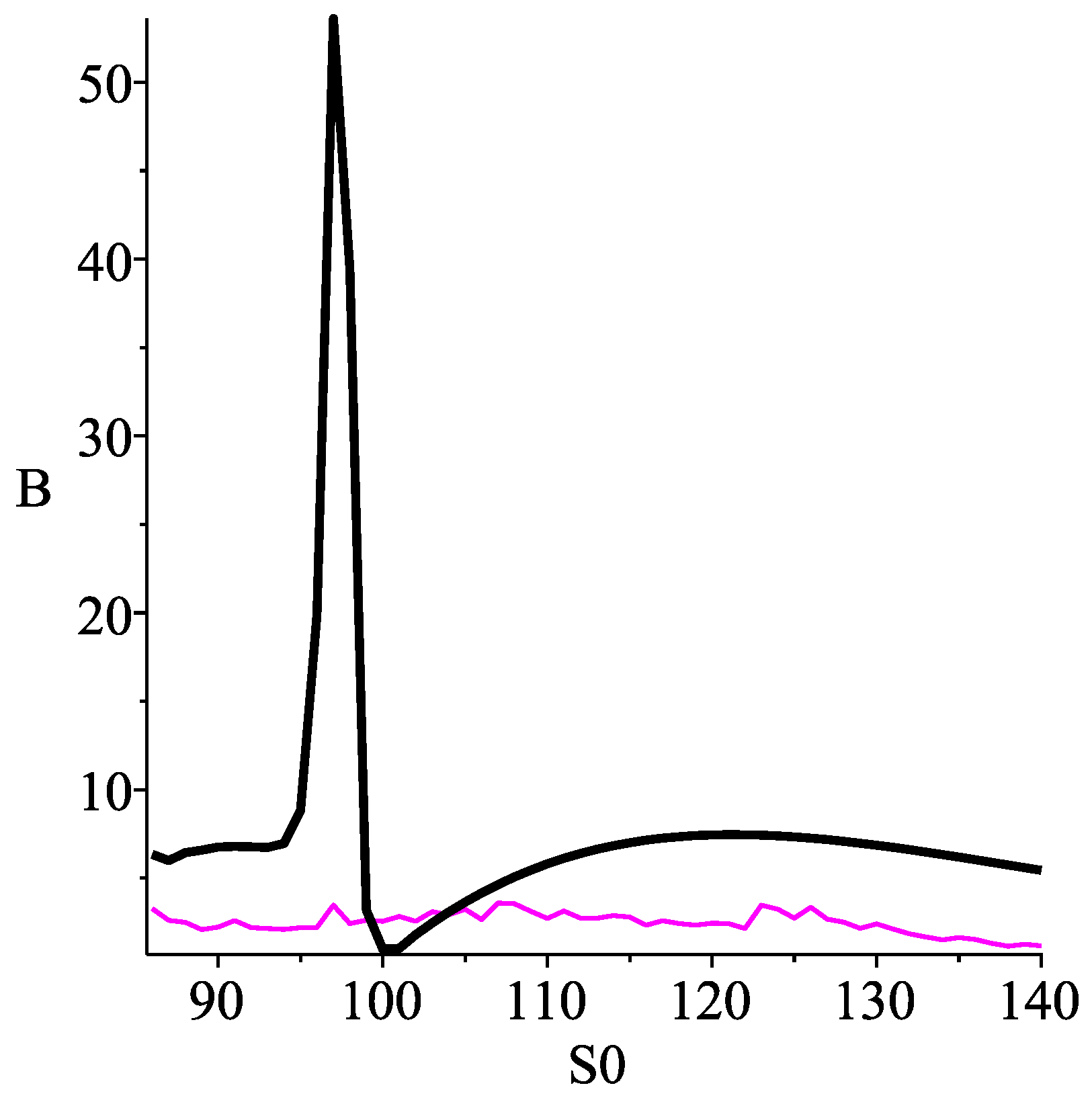
In Figure 3, we zoom in and display only the curves for Joshi’s original split tree (in bold) and the optimal split tree near . We note that, except in a very small interval around the strike, the values of for Joshi’s original split tree are larger than those in the optimal split tree near . On average the value of in Joshi’s original split tree is times the value of in the optimal split tree near . Given , Lemma 2 can be used to translate the quotient of the values of in the two models into a measure of the relative computational effort required by both models. In this measure we obtain that, on average, over the values of , the computational effort used for Joshi’s original split tree is times as much as the computational effort used for the optimal split tree near . Said another way, the optimal split tree near is on average faster than Joshi’s original tree.
More strikingly, unlike Joshi’s original tree, the optimal split tree near does not exhibit a huge spike in the value of for some unfavorable spot prices . If we define
then the value of in Joshi’s original split tree is , and it is in the optimal split tree near . This gives a quotient of . Hence if for every , n is chosen in such a way that , in order to guarantee that, uniformly in , n is large enough to insure an error smaller than , then Lemma 2 says that the optimal split tree near results in calculations which are times faster than in Joshi’s original split tree.
6. Conclusions
In this paper we introduced a flexible version of Joshi’s original split tree and we developed the corresponding convergence theory in the European case. Our flexible split trees are characterized by two additional parameters: the drift and the split time. This allowed us to define optimal values of these parameters under different constraints. For European options, we found an explicit formula for the coefficients of and in the expansion of the error, and we found closed form formulae for the parameters of our optimal split trees. Numerical results suggest that the optimal split tree near can significantly improve the convergence of Joshi’s original split tree.
Because stock options prices are quoted in the Black–Scholes model, binomial tree methods apply naturally to them, as a numerical method to price them when a closed form formula is not available. However, for real options requiring the modeling for several uncertainty sources, the Monte Carlo approach introduced in Longstaff and Schwartz (2001) can be the best choice (see, for instance, Lomoro et al. (2020), Pellegrino et al. (2019), or Sun et al. (2019)). The finite difference method (see, for instance, Wilmott (1998)) is another broadly used numerical tool to price options. An empirical study in the style of Joshi (2009b) that could compare, analyze, quantify, and contextualize the respective advantages of the Monte Carlo approach, the finite difference method, and the tree method, would be an broad and interesting project.
Author Contributions
Both authors contributed to all aspects of this research. Both authors have read and agreed to the published version of the manuscript.
Funding
This research was funded by the American University of Sharjah Faculty Research Grants FRG16-T-09, FRG18-T-09, and FRG20-S-S83.
Acknowledgments
The paper started to take form in Melbourne, in August 2016, following numerous discussions with Mark Joshi, during a one month visit of the authors. We are greatly indebted to Ralf Korn from whom the idea of this paper originates, and who provided suggestions, advice, and comments at every stage of its writing. Guillaume Leduc thanks the American University of Sharjah for the Faculty Research Grants (FRG16-T-09, FRG18-T-09, FRG20-S-S83) which supported this research. Merima Nurkanovic Hot thanks the Research Center (CM) and the DFG-Research Training Group 1932 at the University of Kaiserslautern for support.
Conflicts of Interest
The authors declare no conflict of interest.
Appendix A. A1 Proofs
Appendix A.1. Proof of Proposition 1
First we recall some notation from Section 3.1, and to shorten expressions we set . We denote by the stochastic process corresponding to a flexible binomial model with drift parameter (see Appendix B), and by is its discounted expectation semigroup operator. Note that corresponds to the CRR case. We denote by the stochastic process corresponding to a split tree model with split time and drift , and by its discounted expectation semigroup operator, which is given by (11). We denote by the discounted expectation semigroup operator of a geometric Brownian motion. denotes the price of a call option in a split model with split time and drift , and denotes the price of the same option in the geometric Brownian motion. Finally, denotes the payoff function of a call option with strike K. Recall that
Let be the number of time steps until the split. Then , and the number of time steps remaining until maturity is . Recall Chang and Palmer’s from (A4) in Appendix B. Now suppose that both and are even. All the nodes of have the form
for some integers . This yields
It is not difficult to see that, regardless of the parity of and , we always have for every possible value of . Recall from (13). With Chang and Palmer’s Theorem A1 and Lemma A2 in Appendix B we obtain that
where
and the term is uniform in . Since,
we get
Note that is bounded away from 0 and that both functions and are infinitely differentiable and when multiplied by , for , their derivatives evaluated at x are also uniformly bounded, for . We obtain from Theorem A2 in Appendix C that
Hence
It follows from Theorem A2 in Appendix C that
Therefore
which is exactly what we wanted to prove.
Appendix A.2. Proof of Theorem 1
Recall that denotes geometric Brownian motion and that is its discounted expectation semigroup operator. To shorten the expressions, set . We already have a closed form formula for the term in (18). We need an explicit expression for
where
Recall that,
where is a standard normal random variable. Note that
where
We write in the form
with
On the other hand, with
we get
In this notation,
With Gaussian integrals we obtain
Tedious but otherwise trivial algebraic manipulations yield
Appendix A.3. Proof of Lemma 2
Fix . Under our assumption on the choice of n, we need in model i, with n rounded up. However, the total number of fundamental steps in calculating a tree is equal to the total number of nodes in the tree which is polynomial of degree 2. Let be this polynomial. Then the quotient of the required effort in model 1 over the effort in model 2 is
Appendix B. Flexible Binomial Tree
Let be the fractional part of x, and define and as
Moreover, set
and
Recall that in the flexible binomial model with drift parameter ,
Theorem A1
(Chang and Palmer (2007)). In the flexible model with bounded drift parameter , the value of a call option with spot price , strike price K, risk free rate r, volatility σ, and maturity T satisfies
where is the value of the same option in the Black–Scholes model and
where
Now let
The quantities and are connected through the relation
The quantity is what drives the oscillations in the coefficients of the expansion of the error in Chang and Palmer’s formula (A6). The quantity serves the same purpose in the equivalent formula in Diener and Diener (2004). Leduc (2016b) provides and explicit expressions for the coefficient of in the expansion of the error of the call options in a binomial model where and p are given by
The special case of the CRR model corresponds to in the flexible model and to in Leduc (2016b). Both Chang and Palmer (2007) and Leduc (2016b) are special cases of Diener and Diener (2004), and thus, although expressed in different notation, the formulae in all three papers coincide in the CRR case. We also refer to Huang (2011) where an explicit formula for the coefficient of is found.
Lemma A1.
In the CRR case, if or , or equivalently or , then the term in (A6) can be replaced by .
Proof.
This follows trivially by replacing by 0 or in the formula for the third coefficient of the expansion of the error provided in (Leduc 2016b, p. 1332), together with , which corresponds to the CRR case. ☐
Assume that or . If is a parameter of the CRR model, that is, if is or any combination of them, then we say that the term in (A6), which depends on , is ”uniform in “ if
Lemma A2.
In the CRR case, if or , or equivalently or , the term in (A6) can be replaced by , and moreover, it is uniform in .
Proof.
It was already pointed out in Leduc (2016b) that the O-terms in the asymptotic expansion of the error in powers of are uniform in most parameters, providing that these parameters stay in a closed bounded interval and that also remains bounded. Following the argument in Diener and Diener (2004), the proof of uniformity in is similar to the proof of uniformity in . Only trivial modifications are required. The key here is that, as noted in (Leduc 2016b, p. 1342), all terms of the expansion of the error are factored by where is defined by Diener and Diener as the coefficient of in the expansion of
in powers of . In the CRR case, this gives . The term
guarantees in a straightforward manner that, in the argument in Diener and Diener (2004), one can take the supremum over all values of . ☐
Appendix C. Error Expansion for Very Smooth Payoff Functions
Here again the risk free rate r, the volatility , the spot price , and the maturity T are fixed. Recall the flexible models from Appendix B. We denote by the stochastic process corresponding to a flexible binomial model with drift parameter , and by its discounted expectation semigroup operator. denotes geometric Brownian motions, and denotes the corresponding discounted expectation semigroup operator. We consider European options with maturity T and payoff functions depending on the number of time-steps n. For every time step , we define1 , the error at maturity given that the spot price is x, as
We also define the identity function , and we set . From Leduc (2013), and in a more general setting in Leduc (2016a) where the proof is detailed, we have
where
The following is an extension of Theorem 3.1 in Leduc (2013). It shows that when the payoff functions are uniformly very smooth, the -term in the expansion of the error is rather than .
Theorem A2.
Suppose that payoff functions , , are 9 times continuously differentiable and such that, for , is uniformly bounded. Let be a multiple of , and assume that . Then
where .
Proof.
This is an adaptation of a reasoning in Leduc (2013). Here the payoff functions are very smooth, and the maturity, , is allowed to float within the interval . Note that we can write , for some integer . Then each time step until maturity has the form . It follows from Theorem 2.1 in Leduc (2013) and the commutativity and semigroup properties of , that for every integers , the error at any time step can be localized into single time-step errors:
Additionally, since , this is the same as
Using the assumption that is uniformly bounded, and the fact that we obtain that
Note that this equation is trivial when , since . Specializing with and , for , we see that
Putting this back into (A12) and using we get
Using the well known formula for the sum of the first integers, , yields
Since is uniformly very smooth, it is easy to see that
Because , this gives
References
- Amin, Kaushik, and Ajay Khanna. 1994. Convergence of American option values from discrete-to continuous-time financial models. Mathematical Finance 4: 289–304. [Google Scholar] [CrossRef]
- Bock, Alona, and Ralf Korn. 2016. Improving convergence of binomial schemes and the Edgeworth expansion. Risks 4: 15. [Google Scholar] [CrossRef] [Green Version]
- Broadie, Mark, and Jerome Detemple. 1996. American option valuation: New bounds, approximations, and a comparison of existing methods. The Review of Financial Studies 9: 1211–50. [Google Scholar] [CrossRef] [Green Version]
- Carbone, Raffaella. 2004. Binomial approximation of Brownian motion and its maximum. Statistics and Probability Letters 69: 271–85. [Google Scholar] [CrossRef]
- Carr, Peter, Robert Jarrow, and Ravi Myneni. 1992. Alternative Characterizations of American Put Options. Mathematical Finance 2: 87–106. [Google Scholar] [CrossRef]
- Chan, Jiun Hong, Mark Joshi, Robert Tang, and Chao Yang. 2009. Trinomial or binomial: Accelerating American put option price on trees. Journal of Futures Markets 29: 826–39. [Google Scholar] [CrossRef]
- Chance, Don M. 2008. A synthesis of binomial option pricing models for lognormally distributed assets. Journal of Applied Finance 18: 38–56. [Google Scholar] [CrossRef]
- Chang, Lo-Bin, and Ken Palmer. 2007. Smooth convergence in the binomial model. Finance and Stochastics 11: 91–105. [Google Scholar] [CrossRef]
- Chen, Ting, and Mark S. Joshi. 2012. Truncation and acceleration of the Tian tree for the pricing of American put options. Quantitative Finance 12: 1695–708. [Google Scholar] [CrossRef]
- Chriss, N. 1996. Black-Scholes and Beyond: Option Pricing Models. New York: McGraw-Hill. [Google Scholar]
- Cox, John C., Stephen A. Ross, and Mark Rubinstein. 1979. Option pricing: A simplified approach. Journal of Financial Economics 7: 229–63. [Google Scholar] [CrossRef]
- Diener, Francine, and Marc Diener. 2004. Asymptotics of the price oscillations of a European call option in a tree model. Mathematical Finance 14: 271–93. [Google Scholar] [CrossRef]
- Grosse-Erdmann, Karl, and Fabien Heuwelyckx. 2016. The pricing of lookback options and binomial approximation. Decisions in Economics and Finance 39: 33–67. [Google Scholar] [CrossRef] [Green Version]
- Heuwelyckx, Fabien. 2014. Convergence of European lookback options with floating strike in the binomial model. International Journal of Theoretical and Applied Finance 17: 1450025. [Google Scholar] [CrossRef] [Green Version]
- Huang, K. M. 2011. Analysis of Higher Order Error in the Binomial Model. Master’s Thesis, National Taiwan University, Taipei, Taiwan. [Google Scholar]
- Hull, John, and Alan White. 1988. The use of the control variate technique in option pricing. Journal of Financial and Quantitative Analysis 23: 237–51. [Google Scholar] [CrossRef]
- Jarrow, Robert A., and Andrew T. Rudd. 1983. Option Pricing. Homewood: Richard D Irwin. [Google Scholar]
- Jarrow, Rober A., and Stuart McLean Turnbull. 2000. Derivative Securities. Cincinnati: South-Western Pub. [Google Scholar]
- Jiang, Lishang, and Min Dai. 2004. Convergence of binomial tree methods for european/american path-dependent options. SIAM Journal on Numerical Analysis 42: 1094–109. [Google Scholar] [CrossRef] [Green Version]
- Joshi, Mark S. 2009a. Achieving smooth asymptotics for the prices of European options in binomial trees. Quantitative Finance 9: 171–76. [Google Scholar] [CrossRef]
- Joshi, Mark S. 2009b. The convergence of binomial trees for pricing the American put. The Journal of Risk 11: 87–108. [Google Scholar] [CrossRef]
- Joshi, Mark S. 2010. Achieving higher order convergence for the prices of European options in binomial trees. Mathematical Finance 20: 89–103. [Google Scholar] [CrossRef]
- Joshi, Mark S. 2012. On the analytical/numerical pricing of American put options against binomial tree prices. Quantitative Finance 12: 17–20. [Google Scholar] [CrossRef]
- Korn, Ralf, and Stefanie Müller. 2013. The optimal-drift model: An accelerated binomial scheme. Finance and Stochastics 17: 135–60. [Google Scholar] [CrossRef]
- Lamberton, Damien. 1993. Convergence of the critical price in the approximation of american options. Mathematical Finance 3: 179–90. [Google Scholar] [CrossRef]
- Lamberton, Damien. 1998. Error estimates for the binomial approximation of American put options. Annals of Applied Probability 8: 206–33. [Google Scholar] [CrossRef]
- Lamberton, Damien. 2002. Brownian optimal stopping and random walks. Applied Mathematics and Optimization 45: 283–324. [Google Scholar] [CrossRef]
- Lamberton, Damien. 2018. On the binomial approximation of the American put. Applied Mathematics & Optimization, 1–34. [Google Scholar]
- Leduc, Guillaume, and Ken J. Palmer. 2019. Path independence of exotic options and convergence of binomial approximations. Journal of Computational Finance 23: 73–102. [Google Scholar] [CrossRef]
- Leduc, Guillaume. 2013. A European option general first-order error formula. The ANZIAM Journal 54: 248–72. [Google Scholar] [CrossRef] [Green Version]
- Leduc, Guillaume. 2016a. Option convergence rate with geometric random walks approximations. Stochastic Analysis and Applications 34: 767–91. [Google Scholar] [CrossRef]
- Leduc, Guillaume. 2016b. Can high-order convergence of European option prices be achieved with common CRR-type binomial trees? Bulletin of the Malaysian Mathematical Sciences Society 39: 1329–42. [Google Scholar] [CrossRef]
- Leisen, D. P. J., and M. Reimer. 1996. Binomial models for option valuation-examining and improving convergence. Applied Mathematical Finance 3: 319–46. [Google Scholar] [CrossRef]
- Lin, Jhihrong, and Ken Palmer. 2013. Convergence of barrier option prices in the binomial model. Mathematical Finance 23: 318–38. [Google Scholar] [CrossRef]
- Longstaff, Francis A., and Eduardo S. Schwartz. 2001. Valuing American options by simulation: A simple least-squares approach. The Review of Financial Studies 14: 113–47. [Google Scholar] [CrossRef] [Green Version]
- Lomoro, Antonella, Giorgio Mossa, Roberta Pellegrino, and Luigi Ranieri. 2020. Optimizing risk allocation in public-private partnership projects by project finance contracts. the case of put-or-pay contract for stranded posidonia disposal in the municipality of bari. Sustainability 12: 806. [Google Scholar] [CrossRef] [Green Version]
- Pellegrino, Roberta, Nicola Costantino, and Danilo Tauro. 2019. Supply chain finance: A supply chain-oriented perspective to mitigate commodity risk and pricing volatility. Journal of Purchasing and Supply Management 25: 118–33. [Google Scholar] [CrossRef]
- Staunton, Mike. 2005. Efficient estimates for valuing American options. The Best of Wilmott 2: 91–97. [Google Scholar]
- Sun, Hui, Shuhua Jia, and Yuning Wang. 2019. Optimal equity ratio of bot highway project under government guarantee and revenue sharing. Transportmetrica A: Transport Science 15: 114–34. [Google Scholar] [CrossRef]
- Tian, Yisong. 1993. A modified lattice approach to option pricing. Journal of Futures Markets 13: 563–77. [Google Scholar] [CrossRef]
- Tian, Yisong. 1999. A flexible binomial option pricing model. Journal of Futures Markets 19: 817–43. [Google Scholar] [CrossRef]
- Trigeorgis, Lenos. 1991. A log-transformed binomial numerical analysis method for valuing complex multi-option investments. Journal of Financial and Quantitative Analysis 26: 309–26. [Google Scholar] [CrossRef]
- Van Den Berg, Imme, and F. Koudjeti. 2000. Principles of Infinitesimal Stochastic and Financial Analysis. Singapore: World Scientific. [Google Scholar]
- Walsh, John B. 2003. The rate of convergence of the binomial tree scheme. Finance and Stochastics 7: 337–61. [Google Scholar] [CrossRef]
- Wilmott, Paul. 1998. Derivatives: The theory and Practice of Financial Engineering. Chichester: John Wiley & Sons. [Google Scholar]
| 1 |
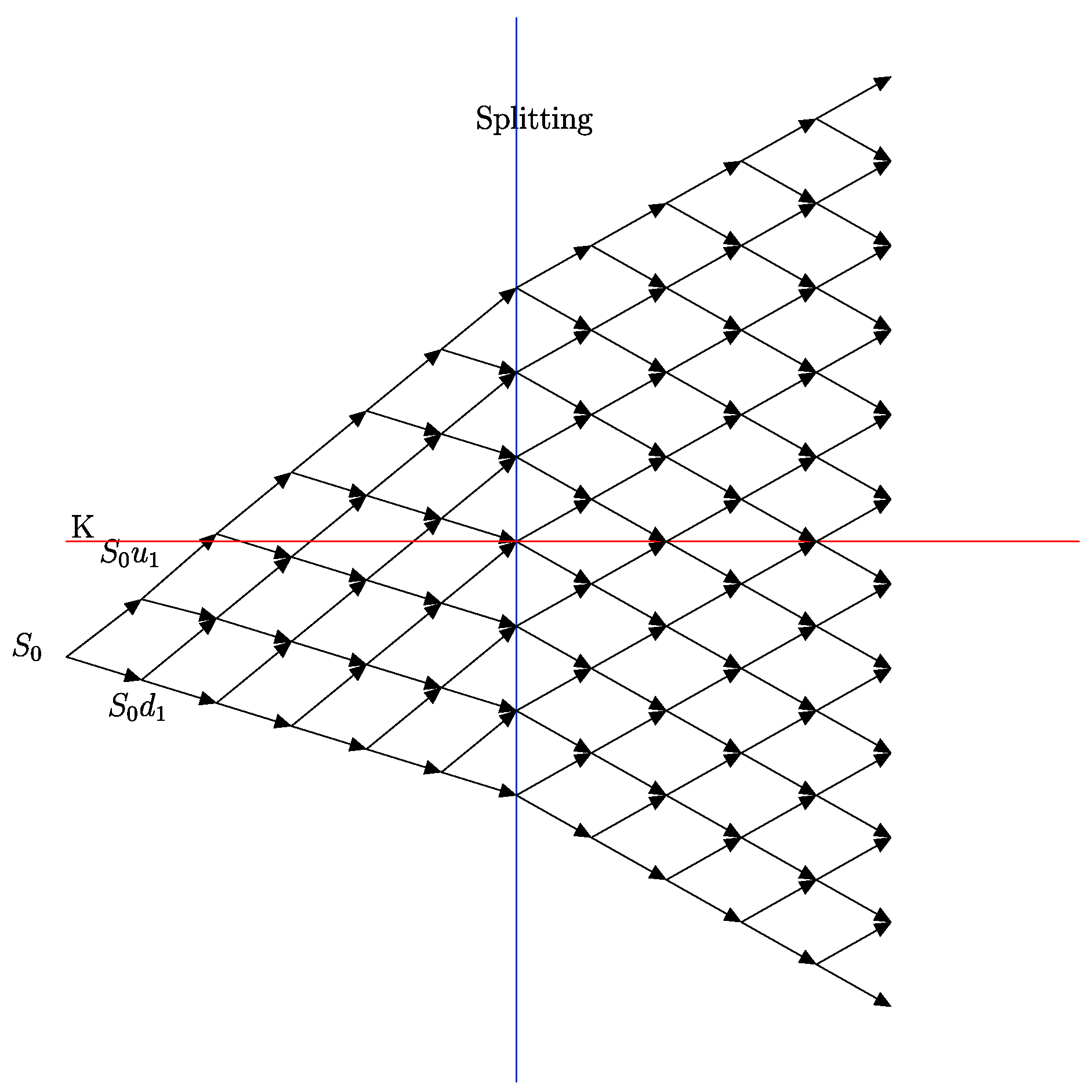
Figure 1.
Values of the split tree in the log-space for Joshi’s original split tree. Here , and from time step onward, the tree is centered around the strike K.
Figure 1.
Values of the split tree in the log-space for Joshi’s original split tree. Here , and from time step onward, the tree is centered around the strike K.

Figure 2.
The value of as a function of , for all the optimal models.

Figure 3.
The value of as a function of , for Joshi’s original split tree (bold) and the the optimal split tree near .
Figure 3.
The value of as a function of , for Joshi’s original split tree (bold) and the the optimal split tree near .

© 2020 by the authors. Licensee MDPI, Basel, Switzerland. This article is an open access article distributed under the terms and conditions of the Creative Commons Attribution (CC BY) license (http://creativecommons.org/licenses/by/4.0/).
Share and Cite
MDPI and ACS Style
Leduc, G.; Nurkanovic Hot, M. Joshi’s Split Tree for Option Pricing. Risks 2020, 8, 81. https://0-doi-org.brum.beds.ac.uk/10.3390/risks8030081
AMA Style
Leduc G, Nurkanovic Hot M. Joshi’s Split Tree for Option Pricing. Risks. 2020; 8(3):81. https://0-doi-org.brum.beds.ac.uk/10.3390/risks8030081
Chicago/Turabian StyleLeduc, Guillaume, and Merima Nurkanovic Hot. 2020. "Joshi’s Split Tree for Option Pricing" Risks 8, no. 3: 81. https://0-doi-org.brum.beds.ac.uk/10.3390/risks8030081
Note that from the first issue of 2016, this journal uses article numbers instead of page numbers. See further details here.