Observable Cyber Risk on Cournot Oligopoly Data Storage Markets


1
RISE Research Institutes of Sweden, P.O. Box 1263, SE-164 29 Kista, Sweden
2
KTH Royal Institute of Technology, SE-100 44 Stockholm, Sweden
3
Department of Mathematics, Uppsala University, P.O. Box 480, SE-751 06 Uppsala, Sweden
4
Länsförsäkringar, SE-106 50 Stockholm, Sweden
*
Author to whom correspondence should be addressed.
Risks 2020, 8(4), 119; https://0-doi-org.brum.beds.ac.uk/10.3390/risks8040119
Submission received: 26 August 2020
/
Revised: 23 October 2020
/
Accepted: 9 November 2020
/
Published: 12 November 2020
(This article belongs to the Special Issue Cyber Risk and Security)
Abstract
:With the emergence of global digital service providers, concerns about digital oligopolies have increased, with a wide range of potentially harmful effects being discussed. One of these relates to cyber security, where it has been argued that market concentration can increase cyber risk. Such a state of affairs could have dire consequences for insurers and reinsurers, who underwrite cyber risk and are already very concerned about accumulation risk. Against this background, the paper develops some theory about how convex cyber risk affects Cournot oligopoly markets of data storage. It is demonstrated that with constant or increasing marginal production cost, the addition of increasing marginal cyber risk cost decreases the differences between the optimal numbers of records stored by the oligopolists, in effect offsetting the advantage of lower marginal production cost. Furthermore, based on the empirical literature on data breach cost, two possibilities are found: (i) that such cyber risk exhibits decreasing marginal cost in the number of records stored and (ii) the opposite possibility that such cyber risk instead exhibits increasing marginal cost in the number of records stored. The article is concluded with a discussion of the findings and some directions for future research.
Keywords:
Cournot market; oligopoly; market concentration; cyber risk; data breach; digital services1. Introduction
With the growth of very large, global digital service providers, recent years have seen increasing concerns about digital oligopolies or monopolies and their potentially harmful effects on for instance competition, the labor market, entrepreneurship and consumer rights (Autor et al. 2020; de Reuver et al. 2018; Kenney and Zysman 2016; Kerber 2016). So profound are the possible ramifications, that The Economist named competition a subject where “economists are rethinking the basics” in the inaugural piece in a series on such issues (Economist 2020). Furthermore, competition in digital services is a top priority of political decision-makers. On 29 July 2020, the CEOs of Amazon, Alphabet (Google’s parent company), Apple, and Facebook were summoned to a much publicized hearing before the US Congress House Judiciary Subcommittee on Antitrust, Commercial, and Administrative Law.1
One particular concern related to market concentration in digital services is cyber security—broadly speaking, the risk that information stored and used in digital systems will be seen by the wrong eyes (confidentiality), be manipulated by the wrong hands (integrity), or not be there when needed (availability). Though the relation between market concentration and cyber security has perhaps received less attention in the public debate, it is at the top of minds of insurers and reinsurers, to whom it represents an important part of the accumulation risk accepted when underwriting the cyber risks of their insureds. The Geneva Association has described accumulation risk as being “at the heart of many concerns about cyber risk”.2
It is not difficult to understand why market concentration in digital services might entail greater accumulation risk to insurers: if many insureds depend on the same digital service provider and that provider experiences a cyber incident, then there will be many claims at the same time, increasing the insurer’s risk, possibly dramatically. A study from 2018, commissioned by Lloyd’s, considered scenarios where major cloud service providers (Google, Amazon, Microsoft, or IBM) experienced interruptions of some 3–6 days. The resulting total ground-up losses were between $6.9 and $14.7 billion and between $1.5 and $2.8 billion in industry insured losses in the US alone (Lloyd’s 2018). Such scenarios raise serious questions about putting all the proverbial eggs in the same basket.
It is the intersection of these important concerns—market concentration and cyber risk—that motivates this paper. More precisely, we are inspired by a recent analysis by Geer et al. (2020), who carefully discuss the relation between market concentration and cyber risk, concluding that “there is often a malign association between trends in market concentration and the location and level of cyber risk within the system” (p. 25). Since Geer et al. do not present a formal theory, our aim is to consider one particular part of their argument more closely, formalizing it within the context of Cournot oligopoly theory, and see what consequences can be derived. Embarking on such a formalization necessitates some simplifications; sacrificing some realism to obtain mathematical rigor. Acknowledging this, we find the results sufficiently interesting to make the theory worthwhile, though as with all formal theories, it has to be applied with care and judgment.
The rest of this paper, which is based on the master thesis of the second author, is structured as follows: Section 2 introduces the Cournot oligopoly model extensively, with a focus on the complications brought by strictly concave production cost. Section 3 then develops some theory about what happens when an additional cyber risk cost is introduced onto a Cournot oligopoly market of data storage service providers, proving that some results are related to convex cyber risk cost. Section 4 reviews some evidence of whether cyber risk cost is in fact convex or concave, discusses the implications, and gives some numerical examples. Section 5 concludes the paper and offers some directions for future research.
2. Preliminaries: The Cournot Oligopoly Market
In the following, we introduce the Cournot model of an oligopoly market. This section makes no claims to profound originality, and is based on standard game theory and economics textbooks (Lindahl 2017; Varian 1992). However, some effort has been spent to construct Example 3 as a pedagogical illustration of the difficulties with strictly concave production cost.
In the Cournot model of an oligopoly market, rival firms produce a homogeneous product at production costs that are increasing in the quantity produced. The market determines the price at which the product is sold, modeled by an inverse demand (price) function P that is decreasing in the total quantity of product produced. Each firm maximizes profits by independently choosing its production quantity. The complication, of course, is that the market price depends on the decisions of all the producers. The resulting equilibrium is a Nash equilibrium in quantities, known as a Cournot equilibrium.
Remark 1.
In general, P need not be strictly decreasing, but can have plateaus where it is flat. In such regions, price will be unaffected by production quantities, and, locally, producers will not face a game but a decision-problem. In the remainder of this article, we will ignore this complication and assume that P is strictly decreasing.
To facilitate the analysis of cyber risk to be undertaken in the next section, let the profit of service-provider firm i thus depend on the income from selling storage of records of data at the market price on a market where the total number of records stored by n competitors is and the production cost is . The profit becomes:
For differentiable (in the following, we always assume differentiability as needed, unless otherwise stated) cost functions , first-order conditions for the equilibrium quantities are found by differentiation and setting to zero, as in the following system of equations:
Now, subtract row j from row i. We have:
With identical differentiable convex (affine or strictly convex) cost functions, Equation (3) implies that is the unique solution to these first-order conditions. In the affine case, , so it can be immediately observed that . In the strictly convex case, assume without loss of generality that . Then, by convexity, , which leads to contradiction since the left- and right-hand-sides obtain different signs (recall that P is strictly decreasing so that ). With inequality thus excluded, . It follows that the last line of Equation (2) is , and the optimal quantity can be found by solving any of the previous n lines as a single variable equation:
To verify that the first-order conditions expressed in Equation (2) identify maximum rather than minimum profits, differentiating once more gives the second-order conditions, that must hold:
Example 1.
Let the cost function be linear and let the inverse demand function decrease linearly in until it becomes zero:
Observe that if total production , then any production is a loss, and firm can unilaterally improve by cutting production to . Thus, this is not a Nash equilibrium, and we can conclude that in the vicinity of the Nash equilibrium, .
Differentiating and and plugging into Equation (4), we have the equilibrium quantities:
Verifying the second-order conditions, we have simply:
Turning instead to different convex production cost functions, Equation (3) means that differences in produced quantity are negatively proportional to the differences in marginal production cost, which is very intuitive.
Example 2.
However, when production costs are not increasing convex functions but rather increasing strictly concave, the situation is more complicated. While the simple procedures used above can still be used to find local maximum profit points for the firms if they exist, these points are not necessarily global ones (Muu et al. 2008). Furthermore, as illustrated in the following example, there may be no Nash equilibria, or there may be multiple Nash equilibria—some of which may be symmetric, and some of which may be asymmetric.
Example 3.
Let be as in Example 1, but let the production cost function for all firms be . The production cost is thus an increasing concave function for all permissible production quantities . For ease of exposition, we consider the duopoly case of two firms.
If, for symmetry, it is assumed that , Equation (4) becomes:
Each of the two solutions to this quadratic equation represents a symmetric point where the first-order conditions are met.
If instead it is assumed that , Equation (3) becomes:
Having thus related the two optimal production quantities to each other, we can express either firm’s first order conditions, from Equation (2), as an equation in a single variable:
Here, the two solutions to the quadratic equation (call them and ) together represent a single asymmetric point where the first-order conditions are met.
The second-order conditions for firm i become:
Thus, depending on the values of b and , Equations (10) and (12) may identify minimum, inflection, or maximum points in the profits of the firms.
Now, one complication that can arise is the absence of Nash equilibria. Let and . Equation (10) suggests a single symmetric solution: a double root at zero production. However, the second-order conditions are not met, as . Thus, this is a point of minimum, not maximum, profits. Equation (12) has complex solutions and in this case, there are no Nash equilibria.
Another complication is multiple Nash equilibria. Let and . Equation (10) gives one positive and one negative solution, the latter of which can immediately be discarded, as it involves negative production quantities. The positive solution yields a Nash equilibrium where the duopolists produce each, with the second-order conditions verifying that any infinitesimal unilateral deviation ε decreases profit. (As pointed out by Muu et al. (2008), with concave costs, such a local maximum is not necessarily a global one, but inspecting the reaction curves confirms that in this case, it is.)
However, Equation (12) suggests another solution: , i.e., an asymmetric solution where one firm produces 1 and the other 0. The second-order condition for the ‘dominating’ firm is satisfied as . The second-order condition for the ‘dominated’ firm is . This is actually an inflection point of the ‘auxiliary’ profit function that allows , with an upwards slope for and a downwards slope for . However, as negative production is not allowed, zero production is actually a profit maximum for the dominated firm, and any unilateral (positive) deviation from it causes its profit to go from zero into the negative.
Thus, there are two Nash equilibria in this case: a symmetric one where the two duopolists split the market equally, and an asymmetric one where one duopolist captures the whole market and the other does better not to enter. Unsurprisingly, the profit of the dominating firm in the asymmetric equilibrium () is greater than the profit of a single firm in the symmetric equilibrium (), and is in fact about twice the total market profit in that case (). It is also noteworthy, however, that for consumers, the effects of the asymmetric case are much less dramatic: the asymmetric market price of is higher than the symmetric duopoly market price of , but not by much compared to the effects on profits.
3. Theory of Convex Cyber Risk on Cournot Oligopoly Markets
Having introduced the Cournot model in the previous section, we now consider the introduction of observable cyber risk. As mentioned in the introduction, the motivating concern here is the risk of data breach, which can be very costly to the parties involved. The simplifying assumption of observability means that, just like production cost, the cyber risk is known from the outset and affects market behavior. While this is an obvious simplification, it is a useful starting point, as it allows building a theory which can then be modified to include the more realistic case where cyber risk (just like production cost or inverse demand) is only imperfectly observable.
Let be a differentiable and strictly increasing function () of the number of records R stored, representing the expected cost of data breach. Firm i now instead maximizes the following profit:
We first prove the straightforward result that an affine cyber risk, i.e., a constant marginal cyber risk cost, does not affect the differences between optimal quantities produced.
Proposition 1
(Affine cyber risk). Let the market have an affine inverse demand function and let each firm i have a distinct production cost function . Then the introduction of an affine cyber risk cost function has no effect on the differences between optimal quantities produced compared to the case without cyber risk cost.
Proof.
Differentiating, forming the system of equations, and subtracting row j from row i as before, the denominator in Equation (3) will also include , which is zero by affinity of . □
Remark 2.
Note that in Proposition 1, we do not even have to assume that production cost functions are convex. Concave production cost may well give rise to complications, such as those illustrated in Example 3, but these are the same with or without an affine .
As will be discussed in Section 4, affine cyber risk is probably not the typical case. The more interesting question is: What happens when the marginal cyber risk cost is not constant? Against the background of concerns about market concentration in digital services, it makes sense to investigate whether the presence of a cyber risk cost can increase or decrease the differences between the optimal quantities produced. We now prove that a strictly convex cyber risk, i.e., an increasing marginal cyber risk cost, decreases these differences under certain conditions.
Proposition 2
(Strictly convex cyber risk). Let the market have an affine inverse demand function and let each firm i have a distinct convex production cost function . Let the difference between two production cost functions be affine. Then, the introduction of a strictly convex cyber risk cost function decreases the differences between the optimal quantities produced compared to the case without cyber risk cost, unless this difference is already zero.
Proof.
Differentiating, forming the system of equations, and subtracting row j from row i gives
Since the difference is affine, the derivative of this difference is constant, and it is convenient to write it as a difference of two constants, corresponding to constant marginal production costs: .
First, we note the equivalence . The ⇒ direction follows from Equation (15) since and the remaining numerator must be zero. The ⇐ direction follows from the same argument as in the absence of cyber risk cost: unless , the left- and right-hand sides get different signs. Thus, the difference between the optimal quantities is zero if, and only if, the difference in marginal production cost is zero, whether there is a cyber risk cost or not.
Now, without loss of generality, assume instead that . Assume that . Then, by convexity of , , where . Thus,
So, by contradiction, we know that . Knowing that , by convexity of , , where . Thus,
As seen, the difference between optimal quantities produced (to the left in the inequality in Equation (17)) is smaller than the corresponding difference without a cyber risk cost function (to the right in the inequality in Equation (17)). Note that since is affine, the denominator is constant even as changes. □
Remark 3.
The assumption that the difference between two production cost functions is affine is a restriction. The main intuition behind it is that it covers the cases where the production cost functions themselves are affine; this affinity is preserved under subtraction. However, imposing the affinity requirement on the difference rather than the production cost functions themselves also allows a few further cases that may of interest. One such case is where the production technology is identical but different jurisdictions impose different affine taxes on firms depending on where data are stored. The difference between total production cost is then affine: (affinity preserved under subtraction). Another possible case is when the production technology is affine and firm-specific , but a progressive (i.e., convex) identical tax is imposed on all firms (e.g., to counter market concentration). Again, the difference between total production costs is affine: (affinity preserved under subtraction).
This result is intuitive: while a firm with a lower marginal production cost can store more records than its competitor with a higher marginal production cost, an increasing cyber risk marginal cost affecting them offsets this advantage, to some extent.
In Proposition 2, we only require that the cyber risk cost function be strictly convex. However, if is also everywhere twice differentiable (on the open interval between end-points), its first derivative is continuous at the end-points, and is either convex or concave, the magnitude of the difference between optimal quantities produced by different firms can be bounded by use of the mean-value theorem.
Proposition 3
(Strictly convex twice differentiable cyber risk with convex/concave first derivative). Let the market have an affine inverse demand function and let each firm i have a distinct convex production cost function . Let the difference between two production cost functions be affine and non-zero. Then, for a strictly convex cyber risk cost function that is twice differentiable on its entire open interval and has a first derivative that is continuous at the end-points and convex, the differences between two optimal quantities produced is bounded as follows:
If the first derivative is instead concave, the differences between two optimal quantities produced are bounded as follows:
Proof.
Assume without loss of generality that (and equivalently ) as in the proof of Proposition 2. By the mean-value theorem, there exists some , such that . With convex , , so . Conversely, with concave , , so . The results follow from plugging the inequalities into Equation (17) and rearranging. We show one of the inequalities in the convex case explicitly (recall that since , to get an upper bound, we add the smallest possible additional term in the numerator):
Note that division by preserves inequalities, since if it were negative, it would imply that , contrary to hypothesis (see also the proof of Proposition 2). The other inequalities follow mutatis mutandis. □
To see why the convexity (or concavity) of is important, consider the case where the convexity of on the interval is unknown. The mean-value theorem still holds, but can be anywhere in the interval, is unknown, and so cannot be used to bound the difference . Knowing that is convex (or concave), however, means knowing that is monotonously increasing (or decreasing) on the interval, meaning that , regardless of its location, can be bounded by the values of at the endpoints, and thus used to bound the difference as well. Furthermore, if is affine, the lower and upper bounds coincide, giving an exact expression:
Corollary 1
(Strictly convex twice differentiable cyber risk with affine first derivative). It follows immediately that if, under the same conditions as in Proposition 3, the first derivative is both convex and concave, i.e., is affine, the second derivative is constant and the exact difference between two optimal quantities is:
Above, we have developed some basic results about convex cyber risk on Cournot data storage markets. Briefly stated, the presence of such convex cyber risk either leaves the market unaffected (constant marginal cyber risk) or decreases the differences between the amount of data stored by each service provider (increasing marginal cyber risk).
However, the possibility of concave cyber risk must also be considered. Concave cyber risk might make overall cost (i.e., the sum of production cost and cyber risk cost) concave as well, or give it a more complicated form with changing convexity properties. As is known from the literature and explained in the previous section, such overall cost might upend the market significantly compared to a situation without cyber risk. In the next section, we therefore examine some empirical evidence of cyber risk cost, and discuss its implications.
Remark 4.
It should be mentioned that the results developed in this section are not per se limited to cyber risk cost, but apply to any additional cost introduced into the Cournot model. However, as will be explained in Section 4, this theory should be particularly relevant to cyber risk.
4. Discussion in Light of Empirical Evidence of Cyber Risk Cost
In recent years, several empirical papers on data breaches have been published. A publicly available source of data is the Privacy Rights Clearinghouse (PRC) Chronology of Data Breaches,3 which is used by, e.g., Edwards et al. (2016); Wheatley et al. (2016); Eling and Loperfido (2017); Xu et al. (2018); and Carfora et al. (2019). However, this PRC data set does not include economic losses, forcing much of the literature to simply use the number of records exposed as the measure of incident severity, or refer to analyses of nonpublic data.
The two most popular such analyses were performed by Jacobs (2014) and Romanosky (2016), respectively. In both cases, the authors find linear relationships between the logarithms of the number of records exposed and the economic loss. For example, according to the regression analysis on nonpublic Ponemon data by Jacobs (2014), losses l from a data breach of r records are described by Equation (22):
Letting and , we can equivalently state that . We immediately observe that this is indeed a cyber risk cost function that is concave in r. Romanosky (2016), with nonpublic Advisen data, investigates more independent regression variables, but finds, with respect to the number of records, a similar model, albeit with a smaller (and, of course, a different constant term). As mentioned, these analyses use nonpublic data, so the validity of the precise models developed are difficult to ascertain. However, the fact that both Jacobs and Romanosky find concave costs () gives strong support for the concavity of data breach cost, even if the exact parameter values remain uncertain.
Should it then be concluded that cyber risk cost is concave in the number of records? It can certainly not be ruled out. However, risk is not just the magnitude l of the loss, but also the probability p that the loss will occur. Clearly, if the probability is constant with respect to the number of records, and the loss is an increasing, concave function, then so is the overall risk. However, what if the probability is not constant, but is affected by the number of records at stake?
Recently, Geer et al. (2020, section 4.2) have convincingly argued precisely this: That highly valuable targets with troves of data are subject to more attacks. Attackers keep trying, meaning that even though the probability of defense against any one attack is high, the joint probability of successful defense against many attacks is smaller. Thus, define a baseline probability that a single attack succeeds, but let the number of attacks suffered be determined by the number of records r at stake, so that the joint probability becomes:
is a parameter governing how attractive the records are to attackers. Using a MacLaurin expansion, the joint probability p can be approximated as follows:
Note that Equation (24) is not valid for too large . As r might span many orders of magnitude (from a small customer database with a few dozens of customers, to the Facebook user database with data on billions of individuals), the approximation only applies for small enough with respect to r.
Here, it should immediately be recognized that Equation (23) assumes that multiple attacks are independent. There are at least two reasonable arguments for this assumption: First, if attackers do indeed try over and over again to get past the defenses of high value targets, it is reasonable to assume that they tweak their means of attack somewhat after each failure. Second, even if lazy attackers do not bother to consciously tweak attacks, conditions will be different anyway, as the number of states that any realistic target can be in is very, very large, and it is highly improbable that the target remains in any one state for very long. Thus, a repeated attack is unlikely to be just a deterministic replay of the previous attack (which would end the same way). Instead, it is reasonable to perceive each attack as a new trial under different conditions (even though the differences may be very small).
We are now in the position to construct a simple model of the observable cyber risk cost of a digital service provider. To do so, recall first that the cost of data breaches discussed above pertain to the owners of the data (not their service-providers) and second that observable risk in this context means that it is known from the outset and affects market behavior. This means that if the cyber risk of a service-provider indeed increases with the total number of records stored with that provider, that provider will have to lower the price or, equivalently, reimburse customers for losses to remain competitive. Otherwise, the customers will go to someone storing fewer records (from other customers), being a less attractive target.
Given these assumptions and the Jacobs (2014) regression, the observable cyber risk cost of a service provider i that stores records on behalf of its m customers becomes:
To be able to work with the cyber risk cost as a function of all records stored rather than as a function of the m-element vector , it is convenient to bound by a best case, lowest cyber risk (a single customer owns all records) and a worst case, highest cyber risk (m customers each owning just a single record each). Letting , we have:
Here, to the left, the sums in Equation (25) contain just a single term, and to the right, all the , since all .
Whether (Jacobs 2014) or (Romanosky 2016), we see that the convexity conditions on posed in Propositions 2 and 3 are met. Furthermore, in the worst case, the additional condition posed in Corollary 1 is also met, as and .
Example 4.
Let be as in Example 1, , as in the worst case described above, and let the service providers have different linear production cost functions , such that , i.e., so that each of their marginal production costs is an integer multiple of c.
With strictly convex total cost (production cost plus cyber risk cost), we know that there is a single Nash equilibrium, and by Corollary 1, we immediately know that in this equilibrium:
Given the particular production cost structure, we can find , the difference in optimal production quantities between consecutive firms:
Total production can now be found as an arithmetic sum, starting from the production of the n:th firm with the greatest production cost and adding one for each firm until the first firm with the smallest production cost is reached:
can then be found to be solving the first order conditions of firm n, i.e., by differentiating Equation (14) and setting it to zero:
Once is known, the corresponding problem for any of the other firms can also be solved by adding the appropriate number of :
Example 4 was selected for its analytical tractability, where the particular production cost structure was selected so that the arithmetic sum allows us to find exact solutions. However, in the best case (and indeed all the more realistic cases in-between), the first-order conditions form a non-linear system of equations, where the difference is not constant, despite constant differences in marginal production cost, but depends on R. More precisely, subtracting row j from row i in the best case, we have:
In the following example, we contrast numerical solutions of the best case (Equation (32) and ) with the analytical solutions of the worst case (as in Example 4) and the baseline case with no (observable) cyber risk (as in Example 2).
Example 5.
Let be as in Example 1, let the production costs of the service providers be as in Example 4, and consider three different cyber risk cost functions : The worst and best cases, respectively, from Equation (26) (both convex), and no (observable) cyber risk at all as a baseline. As in Example 4, the total cost (production cost plus cyber risk cost) is convex in all three cases, so we know that each has a a single Nash equilibrium.
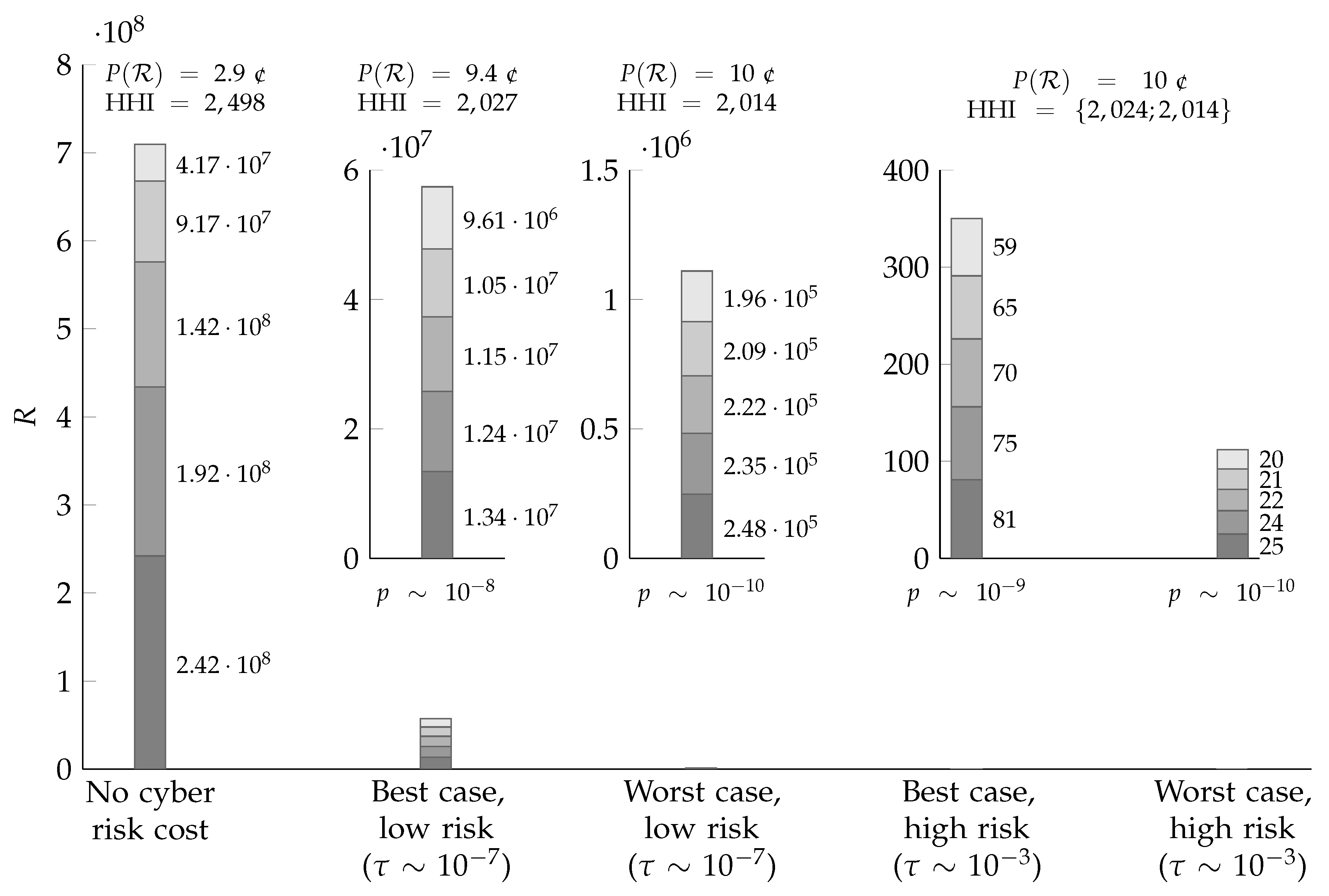
To construct a reasonably realistic example, let there be firms, and let , , and . Furthermore, following Jacobs (2014), let and .
In Figure 1, the optimal numbers of records stored by the five firms are compared in different scenarios, along with the market price per record expressed in cents (1 ¢—the Jacobs regression being in dollars). Recall that the price is a gross price—as remarked above, the observability of cyber risk costs means that each firm also has to offer a discount or reimbursement to compensate for the cyber risk costs entailed by storing a large amount of records. The ‘no cyber risk cost’ scenario is the baseline case. In the ‘low risk’ scenario, , so that . In the ‘high risk’ scenario, , so that .
Figure 1 illustrates the theory developed in Section 3: First, the presence of cyber risk restricts optimal quantities, so that fewer records are stored than in the baseline case. Second, this effect is greater in the worst case than in the best case. Third, the difference between the optimal numbers of records stored decreases in the presence of cyber risk. To illustrate this, the Herfindahl–Hirschman Index (HHI), a common measure of market concentration, is shown in the figure. The HHI is the sum of the squares of each firm’s market share expressed as a percentage (Hirschman 1964). With five firms, it thus ranges from (perfect monopoly) to 2000 (five equal shares). As seen in Figure 1, the presence of observable cyber risk pushes the market towards much more equal shares (of a much smaller market). Whereas firm 1 (marginal cost c) stores almost six times the number of records of firm 5 (marginal cost ) in the ‘no cyber risk cost’ scenario, observable cyber risk almost completely removes this advantage. Intuitively, this can be understood, since production cost, as a share of total cost, decreases relative to cyber risk cost.
The effect depicted in Figure 1 is dramatic—hence the need to use separate inset plots with different axis scales. From storing some 700 million records of data in the absence of observable cyber risk, the market collapses to storing some 60 million (best case) or just a single million (worst case) records in the low risk scenario. By Equation (24), the corresponding breach probability p is in the order of for the number of records stored in the best case, and in the order of for the number of records stored in the worst case.
The even more dramatic collapse in the high risk scenario, where the number of records stored is just a few hundred, compensates for the increase in , so that the resulting probabilities of breach p for the (minuscule) number of records stored are the same for the worst case and an order of magnitude smaller in the best case.
To put these probabilities in context, it should be mentioned that the ‘high risk’ scenario was deliberately designed so that the breach probability for the largest service provider in the ‘no cyber risk cost’ baseline would become if cyber risk would suddenly become observable. A probability in the order of one per cent is aligned with the approximate ratio of cyber insurance premiums to indemnity limits (Franke 2017), giving a hint of how the insurance market assesses this probability. In, the ‘low risk’ scenario, by contrast, the corresponding breach probability for the largest service provider is four orders of magnitude smaller, about .
It should be stressed that Example 5 is just an example. The numerical values must be taken with a large grain of salt, as must the dramatic quantitative impact of (observable) cyber risk found. Nevertheless, the example, and the broader discussion in this section, highlight the importance of further empirical investigation. The next section summarizes the conclusions of the paper and suggests such future work.
5. Conclusions and Outlook
Against the background of growing concerns about both (i) oligopolies in digital services and (ii) cyber security and market concentration, the previous sections have developed some theory about how convex cyber risk affects Cournot oligopoly markets of data storage. We have shown that with constant or increasing marginal production cost, the addition of increasing marginal cyber risk cost decreases the differences between the optimal numbers of records stored by the oligopolists, in effect offsetting the advantage of lower marginal production cost. Furthermore, we have considered the empirical literature on data breach cost, finding both (i) the prima facie possibility that such cyber risk exhibits decreasing marginal cost in the number of records stored and (ii), by the elaboration of an argument originally made by Geer et al. (2020), the opposite possibility that such cyber risk instead exhibits increasing marginal cost in the number of records stored.
These results open several interesting possibilities:
- If data storage production cost is convex (with constant or increasing marginal production cost), then (sufficiently) concave cyber risk cost may turn the resulting Cournot market into the complicated case where no, a single, or multiple Nash equilibria may exist. Prima facie concavity of cyber risk cost is very possible.
- If data storage production cost is convex (with constant or increasing marginal production cost), then convex cyber risk cost will instead make oligopolists with different marginal production costs more equal, offsetting the advantage of a low marginal production cost. Such convex cyber risk cost is also very possible, if more data stored attracts more attacks.
- If data storage production cost is instead concave (with economies of scale implying decreasing marginal production cost) as is certainly possible, then (sufficiently) convex cyber risk cost may turn the resulting Cournot market into the straightforward, single Nash equilibrium case, if the total cost becomes convex.
- More generally, combinations of convex or concave production and cyber risk costs may produce a total cost that is (globally) convex or concave, or one that changes convexity, so that it is (locally) sometimes convex, sometimes concave. On such a market, the existence and uniqueness of Nash equilibria are not guaranteed.
These possibilities call for further empirical investigation. More precisely, at least the following topics deserve more research:
- Data breach cost in general should be further investigated. While current research such as that by Jacobs (2014) and Romanosky (2016) is often based on nonpublic data, public data would be preferable, even though it may be difficult to obtain. With advances in this area, we will have an ever better appreciation of the properties, including the magnitudes of cyber losses.
- Convexity properties of data breach cost should be given specific attention. In particular, empirical investigation of the circumstances under which more data attracts more attacks are of particular importance to determine the properties of probabilities of cyber losses occurring.
- Convexity properties of non-data breach cyber incident cost, e.g., from business interruption should not be forgotten. Antagonistic business interruption incidents may follow a similar logic to antagonistic data breach—greater actors attract more attacks. However, it is perfectly possible that non-antagonistic business interruption incidents also include amplifying logic, e.g., related to incidents spreading through interconnected information systems (Wang and Franke 2020).
- Convexity properties of data storage production cost also deserve more investigation. While it is clear that the marginal production cost of data storage is close to zero, its convexity properties are not equally clear. This is particularly true if the service produced is not pure storage, but also includes other services further up the value-chain, such as analytics, legal compliance, or cyber warranties (Woods and Simpson 2018).
With a greater understanding of these empirical questions, the practical consequences of the theory set forth in Section 3 and illustrated in Section 4 will become clearer. This is of particular relevance to insurers and reinsurers. To see why, recall that the theory we have developed makes the simplified assumption that cyber risks are fully observable to market actors. However, since this is clearly far from the case in practice, there is a considerable risk that decisions are made as if there were no cyber risks, even though there are. However, if insurers could better observe cyber risks, they have the ability to nudge and incentivize their customers towards less risk. For example, if cyber risk cost is indeed convex in the number of records stored, than insurers might be well advised to raise the premiums for customers storing their data with the largest cloud service providers. Conversely, if cyber risk cost is concave in the number of records stored, those premiums should be lowered instead. Thus, insurers might play an important role in making cyber risk more observable. However, this hinges crucially on more research into the topics listed above.
Two final remarks should be made about how the theory proposed could be made more realistic:
- Risk aversion could be introduced so that actors (service providers, their customers, insurers etc.) do not just care about the expected values of cyber risks, but about their full distribution.
These extensions remain future work.
Author Contributions
Conceptualization, U.F. and A.H.; formal analysis, U.F. and A.H.; writing—original draft preparation, U.F. and A.H.; writing—review and editing, U.F.; visualization, U.F. and A.H.; supervision, U.F.; project administration, U.F.; funding acquisition, U.F. All authors have read and agreed to the published version of the manuscript.
Funding
This research was funded by the Swedish Foundation for Strategic Research, grant no. SM19-0009 (U.F.) and Länsförsäkringar (A.H.).
Acknowledgments
Daniel Woods of the University of Innsbruck read an early draft and made useful comments that improved the manuscript substantially. Additional valuable remarks were made by the three anonymous reviewers.
Conflicts of Interest
The authors declare no conflict of interest. The funders had no role in the design of the study; in the collection, analyses, or interpretation of data; in the writing of the manuscript, or in the decision to publish the results.
References
- Akerlof, George A. 1970. The Market for “Lemons”: Quality Uncertainty and the Market Mechanism. Quarterly Journal of Economics 84: 488–500. [Google Scholar] [CrossRef]
- Autor, David, David Dorn, Lawrence F. Katz, Christina Patterson, and John Van Reenen. 2020. The fall of the labor share and the rise of superstar firms. The Quarterly Journal of Economics 135: 645–709. [Google Scholar] [CrossRef] [Green Version]
- Carfora, Maria Francesca, Fabio Martinelli, Francesco Mercaldo, and Albina Orlando. 2019. Cyber risk management: An actuarial point of view. Journal of Operational Risk 14: 77–103. [Google Scholar] [CrossRef]
- de Reuver, Mark, Carsten Sørensen, and Rahul C. Basole. 2018. The digital platform: A research agenda. Journal of Information Technology 33: 124–35. [Google Scholar] [CrossRef] [Green Version]
- Economist. 2020. A healthy dose of competition: From hospitality to hipsterism. The Economist 436: 53–54. [Google Scholar]
- Edwards, Benjamin, Steven Hofmeyr, and Stephanie Forrest. 2016. Hype and heavy tails: A closer look at data breaches. Journal of Cybersecurity 2: 3–14. [Google Scholar] [CrossRef] [Green Version]
- Eling, Martin, and Nicola Loperfido. 2017. Data breaches: Goodness of fit, pricing, and risk measurement. Insurance: Mathematics and Economics 75: 126–36. [Google Scholar] [CrossRef]
- Franke, Ulrik. 2017. The cyber insurance market in Sweden. Computers & Security 68: 130–44. [Google Scholar] [CrossRef]
- Geer, Dan, Eric Jardine, and Eireann Leverett. 2020. On market concentration and cybersecurity risk. Journal of Cyber Policy 5: 9–29. [Google Scholar] [CrossRef]
- Hirschman, Albert O. 1964. The paternity of an index. The American Economic Review 54: 761–62. [Google Scholar]
- Jacobs, Jay. 2014. Analyzing Ponemon Cost of Data Breach. Data Driven Security. Available online: http://datadrivensecurity.info/blog/posts/2014/Dec/ponemon/ (accessed on 12 December 2019).
- Kenney, Martin, and John Zysman. 2016. The rise of the platform economy. Issues in Science and Technology 32: 61–69. [Google Scholar]
- Kerber, Wolfgang. 2016. Digital markets, data, and privacy: Competition law, consumer law and data protection. Journal of Intellectual Property Law & Practice 11: 856–66. [Google Scholar] [CrossRef] [Green Version]
- Lindahl, Lars-Åke. 2017. Spelteori [Game Theory]. Uppsala University. The Cournot Model Is Treated in Chapter 3 on pp. 51–57. Available online: http://www2.math.uu.se/~lal/kompendier/Spelteori2014.pdf (accessed on 25 March 2020).
- Lloyd’s. 2018. Cloud Down: Impacts on the US Economy. Technical Report, Lloyd’s of London. Available online: https://www.lloyds.com/news-and-risk-insight/risk-reports/library/technology/cloud-down (accessed on 19 March 2018).
- Muu, Le D., V. H. Nguyen, and N. V. Quy. 2008. On Nash–Cournot oligopolistic market equilibrium models with concave cost functions. Journal of Global Optimization 41: 351–64. [Google Scholar] [CrossRef]
- Romanosky, Sasha. 2016. Examining the costs and causes of cyber incidents. Journal of Cybersecurity 2: 121–35. [Google Scholar] [CrossRef] [Green Version]
- Varian, Hal R. 1992. Microeconomic Analysis, 3rd ed. The Cournot model is treated in Chapter 16, primarily on pp. 285–91. New York: WW Norton. [Google Scholar]
- Wang, Shaun S., and Ulrik Franke. 2020. Enterprise IT Service Downtime Cost and Risk Transfer in a Supply Chain. Operations Management Research 13: 94–108. [Google Scholar] [CrossRef] [Green Version]
- Wheatley, Spencer, Thomas Maillart, and Didier Sornette. 2016. The extreme risk of personal data breaches and the erosion of privacy. The European Physical Journal B 89: 1–12. [Google Scholar] [CrossRef] [Green Version]
- Woods, Daniel W., and Andrew C. Simpson. 2018. Cyber-warranties as a quality signal for information security products. In International Conference on Decision and Game Theory for Security. Cham: Springer, pp. 22–37. [Google Scholar] [CrossRef]
- Xu, Maochao, Kristin M. Schweitzer, Raymond M. Bateman, and Shouhuai Xu. 2018. Modeling and predicting cyber hacking breaches. IEEE Transactions on Information Forensics and Security 13: 2856–71. [Google Scholar] [CrossRef]
| 1. | Online Platforms and Market Power, Part 6: Examining the Dominance of Amazon, Apple, Facebook, and Google, House Event 110883, https://www.congress.gov/event/116th-congress/house-event/110883, accessed 21 August 2020. |
| 2. | The Geneva Association, Addressing cyber accumulation risk, 16 August 2018, https://www.genevaassociation.org/addressing-cyber-accumulation-risk, accessed 25 February 2019. |
| 3. |
Figure 1.
Stacked bar plots of optimal number of records stored by five different firms with different marginal production costs under different scenarios. Note that the four risky cases with too small quantities depicted accurately in the main plot are also separately depicted in inset plot.
Figure 1.
Stacked bar plots of optimal number of records stored by five different firms with different marginal production costs under different scenarios. Note that the four risky cases with too small quantities depicted accurately in the main plot are also separately depicted in inset plot.

Publisher’s Note: MDPI stays neutral with regard to jurisdictional claims in published maps and institutional affiliations. |
© 2020 by the authors. Licensee MDPI, Basel, Switzerland. This article is an open access article distributed under the terms and conditions of the Creative Commons Attribution (CC BY) license (http://creativecommons.org/licenses/by/4.0/).
Share and Cite
MDPI and ACS Style
Franke, U.; Hoxell, A. Observable Cyber Risk on Cournot Oligopoly Data Storage Markets. Risks 2020, 8, 119. https://0-doi-org.brum.beds.ac.uk/10.3390/risks8040119
AMA Style
Franke U, Hoxell A. Observable Cyber Risk on Cournot Oligopoly Data Storage Markets. Risks. 2020; 8(4):119. https://0-doi-org.brum.beds.ac.uk/10.3390/risks8040119
Chicago/Turabian StyleFranke, Ulrik, and Amanda Hoxell. 2020. "Observable Cyber Risk on Cournot Oligopoly Data Storage Markets" Risks 8, no. 4: 119. https://0-doi-org.brum.beds.ac.uk/10.3390/risks8040119
Note that from the first issue of 2016, this journal uses article numbers instead of page numbers. See further details here.