Nonparametric Malliavin–Monte Carlo Computation of Hedging Greeks


1
Department of Economics and Management, University of Firenze, 50127 Firenze, Italy
2
Department of Economics and Management, University of Parma, 43125 Parma, Italy
*
Author to whom correspondence should be addressed.
Risks 2020, 8(4), 120; https://0-doi-org.brum.beds.ac.uk/10.3390/risks8040120
Submission received: 12 October 2020
/
Revised: 5 November 2020
/
Accepted: 9 November 2020
/
Published: 13 November 2020
(This article belongs to the Special Issue Computational Methods in Quantitative Risk Management)
Abstract
:We propose a way to compute the hedging Delta using the Malliavin weight method. Our approach, which we name the -method, generally outperforms the standard Monte Carlo finite difference method, especially for discontinuous payoffs. Furthermore, our approach is nonparametric, as we only assume a general local volatility model and we substitute the volatility and the other processes involved in the Greek formula with quantities that can be nonparametrically estimated from a given time series of observed prices.
1. Introduction
In finance, the numerical computation of the option price sensitivities, named Greeks, has attracted much attention in the last few years, as the knowledge of the Greeks and their implementation as risk management tools have paramount importance when trading financial derivatives. However, their numerical computation using the Monte Carlo finite difference method is particularly inefficient in the case when the option payoff is represented by a discontinuous function of the underlying asset, as it is often the case.
In their seminal paper, Fournié et al. (1999) show that the stochastic calculus of variations, also referred as the Malliavin calculus (see Malliavin 1997), is the correct tool for computing hedging Greeks as it allows us to consider the effects of perturbations of the model (e.g., perturbation on the initial data, volatility process, …) on functionals of random variables expressing the payoff. Fournié et al. (1999), (2001) propose to exploit the integration by parts formula based on the Malliavin calculus to avoid computing the derivatives of possibly non differentiable payoff functionals as a strategy to get efficient Monte Carlo methods for computing the Greeks. The integration by parts formula can be performed in different ways, producing alternative weights, which are numerically more or less efficient. Even if the different expressions are equivalent from a mathematical point of view, when performing numerical computations they slightly differ, even if the same random series is used. The problem of the optimality of the weight—i.e., providing the minimal variance—is addressed in Kohatsu-Higa and Monteiro (2001) and Benhamou (2003).
Furthermore, the practical implementation of the Malliavin–Monte Carlo method requires the knowledge of the precise form of the diffusion function of the underlying process—i.e., the latent volatility process. This is a crucial point both for pricing and hedging, as demonstrated by the huge amount of literature on determining the correct specification of the underlying model—see Aït-Sahalia (1996). Moreover, the specification of the functional form of the diffusion function is even harder to determine. In this respect, the use of a nonparametric estimator of the volatility can be substantial in terms of avoiding misspecification of the hedging Greeks. Hedging errors due to model misspecification have been investigated from different points of view—see Bouleau (2003); Hayashi and Mykland (2005) and the references therein.
In this paper, we address both issues. We propose a way to compute the weight in the Malliavin weight method that yields a faster convergence rate. Furthermore, our approach is nonparametric, as we only assume a general local volatility model and we substitute the volatility and the other processes involved in the Greek formula with quantities that can be nonparametrically estimated given the time series of observed prices. This result can be achieved by expressing the weight using the rescaled variation which has been introduced in Barucci et al. (2003); Malliavin and Mancino (2002b).
An important advantage of expressing the Malliavin weight in terms of the rescaled variation relies in the fact that this function satisfies an ordinary differential equation instead of a stochastic differential equation. This result has an impact on the numerical efficiency of the Malliavin–Monte Carlo method. In fact, as long as the method is applied only to the case in which the underlying process is a Black–Scholes model, as in Elie et al. (2007); Fournié et al. (1999), the numerical computation of the weight involves only one Itô integral. Nevertheless, this is a very special case: as the underlying SDE is linear, the linearized SDE for the variation process and for the log-normal process are the same. The situation is drastically different if the underlying model is non-linear, as for the local volatility models as well as for stochastic volatility models. Under these models, the expression of the weight involves more than one stochastic integral. The simplest numerical approximation to these stochastic integrals is given by the Euler–Maruyama method. It is well known that this method has strong order of convergence 0.5 and weak order of convergence 1 for Itô stochastic integrals, while it is of order for Riemann integrals. Therefore, when we consider an underlying model which is not log-normal, Fournié et al. (1999) account for numerically computing a double stochastic integral, while our approach requires us only to compute one stochastic integral.
In this paper, we assume an underlying local volatility model,; namely, we model volatility as a level-dependent quantity (i.e., a deterministic function of the asset price). There are different motivations for this kind of model. For instance, in a single asset, market volatility depends on the asset price and, therefore, the market is complete. Moreover, this way to model asset price volatility is well suited to capture the relationship between volatility and asset price-returns (leverage effect). The simplest way to model the negative relation between asset-price returns and volatility is to assume a constant elasticity of variance (CEV) model—see Cox and Ross (1976). Furthermore, level dependent volatility has also been employed to reproduce the implied volatility smile, see Derman and Kani (1994); Dupire (1994); Hobson and Rogers (1998).
The paper is organized as follows. In Section 2, we describe the Malliavin weight approach to Greek computation and its nonparametric application; moreover, the Black–Scholes model and the CEV model are briefly analyzed. In Section 3, we show the computational advantage of computing the weight function by a single stochastic integral instead of a double stochastic integral; in addition, we show the computational efficiency of the method when compared to the standard finite difference Monte Carlo method. Finally, in Section 4 we illustrate an empirical nonparametric implementation of our approach for the EUR/USD exchange rate options on the period from 29 February 2016 to 3 June 2016. Section 5 concludes. The Appendix A resumes the mathematical computation of the rescaled variation and its model-free expression.
2. Greeks Computation via Malliavin Calculus and the Rescaled Variation
In this section we recall the main ingredients for the computation of the Greeks using the Malliavin calculus, referring to Fournié et al. (1999) and Malliavin and Thalmaier (2006) for details. The underlying asset price is described by a diffusion process whose dynamic is described under the risk neutral probability by the following SDE1
where is a deterministic function of the asset price, r the constant risk-free interest rate and W a Brownian motion on a filtered probability space.
Consider a contingent claim with a payoff function of the form for some function f. The no-arbitrage price of the contingent claim is given by
where E is the expectation under the risk neutral probability and the notation denotes the solution of (1) at time which has initial condition .
From a mathematical point of view, the Greeks formulae are given by the directional variations of in response to a perturbation of the initial datum (in the case of ), of the volatility coefficients (in the case of ) or of different parameters. In the present paper we focus on the computation of , the first derivative of with respect to the initial datum. Consider the variation of the initial condition , for which the is given by
If the expression (3) does not have an explicit-closed formula (because in most cases the distribution of is not known—see Remark 2), we may think of using Monte Carlo simulations in order to compute the expectation. Moreover, as the function f is usually not smooth, we can resort to the computation of difference quotients (i.e., finite differences) to perform the derivative in (3).
Fournié et al. (1999) showed that it is possible to accelerate the rate of convergence of the Monte Carlo method and to overcome the lack of classical differentiability of the payoff function f, if we are able to express the differentiation involved in the Greeks formulae—e.g., (3), as the expectation of the payoff function multiplied by a weight , which does not depend on the payoff function itself. The authors study numerical applications of the method in the case where the volatility is constant, showing its efficiency. We sketch the idea behind this approach.
In the context of stochastic calculus of variation (see Malliavin (1997)), a perturbation of the initial condition propagates along the trajectory W as
where and the process is the rescaled variation defined as the ratio between the variation process associated to (1) and the diffusion coefficient of (1), namely
Remember that the variation process follows an SDE, which is the linearized equation of the SDE (1) driving the price2
Then, we have
where is the Malliavin derivative along the direction h and the last equality is obtained by means of the integration by parts formula (see Malliavin (1997)). The function can be arbitrarily chosen but it must satisfy . For simplicity we will consider .
Therefore, the weight is equal to and it does not depend on the payoff function. Furthermore, formula (7) does not require us to differentiate the payoff function.3
The computation of the weight in (7) is far from being trivial. In fact, it is worth noting that apriori the computation of the weight involves a double stochastic integral, as the rescaled variation is the solution to an SDE. However, in Malliavin and Mancino (2002b); Malliavin and Thalmaier (2006) it is proven that the rescaled variation actually evolves in time according to a linear ordinary differential equation. More precisely, the rescaled variation is differentiable with respect to t and it holds that
where
The general case of this result in stated in Appendix A as Theorem A1.
In practice, the Greeks can be calculated in a parametric framework as follows: first determine a parametric model, as a general diffusion process on the underlying process, that can produce the best fit, and estimate the parameters in the model; then, calculate the Greeks using the selected model. We take a nonparametric approach instead. The function contains terms, such as the volatility function and its derivatives, which are latent and should be estimated from the data. Following Barucci et al. (2003); Malliavin and Mancino (2002b), it can be expressed in terms of three factors which can be estimated nonparametrically given high frequency asset return data using the Fourier methodology introduced by Malliavin and Mancino (2002a, 2009). Therefore, the rescaled variation is expressed by means of quantities which can be empirically estimated using the price process observations. More precisely, the function in (9) can be expressed by means of terms which are iterated cross volatilities. The result is the following:
Denoting by the quadratic (co-)variation operation, define the following cross-volatilities:
then the function in (9) has the following expression
The general case of this result is stated in Appendix A as Theorem A2.
On their turn, these cross volatilities are stochastic functions that can be estimated using the Fourier estimation method—see Mancino et al. (2017). In particular, consistent estimators of the stochastic functions , and have been studied in Mancino and Sanfelici (2020).
The next subsection illustrates the methodology by means of two examples, the first one is the Black–Scholes model, the second is a level dependent volatility model, the Constant Elasticity of Variance (CEV) model.
2.1. Two Examples
We illustrate the methodology first on the Blac-k-Scholes model, then on the CEV model in the case of the European-type options.
2.1.1. The Black–Scholes Model
Under the risk neutral probability, let follow a Black–Scholes model
Note that this is a linear SDE, thus the SDE for coincides with that of , with different initial data
and . Using (7), as in Fournié et al. (1999) we obtain the Delta:
Remark 1.
Note that, for the Black–Scholes model , thus —i.e., constant—which implies that . This can also be derived by using the expression (9).
2.1.2. The CEV Model
Consider now the CEV model for , that is, under the risk neutral probability,
The associated SDE of the variation process is
The non linearity of the diffusion coefficient—i.e., —drastically changes the relation between and . The solution of the linear SDE (13) is
The computation of the Delta using (7), as in Fournié et al. (1999), gives:
which entails the computation of two stochastic integrals.
On the other side, by using the -method, through the formula (8) we get:
which entails the computation of a single stochastic integral.
The computation of for the CEV model can be easily obtained from (9) and is equal to
Remark 2.
Note that even for a plain vanilla call option, there is no explicit expression for the non arbitrage price (and thus the Delta) assuming a CEV model. For the pricing and hedging of options, the available formulae are expressed by a series of incomplete Gamma functions—see, for instance, Davydov and Linetsky (2001) .
3. Simulation Study
The aim of this section is twofold: first we show the computational advantage of computing the weight function by a single stochastic integral as in (15) versus a double stochastic integral as in (14); second, we show the computational efficiency of the method when compared to the standard finite difference Monte Carlo method.
3.1. Computation of the Weight
As a case study, we consider the CEV model. We compare two alternative ways to compute the Malliavin weight, namely by the processes
and
Equation (18) exploits the knowledge of the price-volatility feedback rate , and requires the computation of a Riemann integral, while the term (17) involves the computation of a stochastic integral.
The simplest numerical approximation to these stochastic processes is given by the Euler–Maruyama method. It is well known that this method has strong order of convergence 0.5 and weak order of convergence 1. Although the Delta values in (14) and (15) are expressed as expected values, it is important to quantify the ability of the method to compute strong (i.e., pathwise) solution on average, because this reflects on the weak convergence as well.
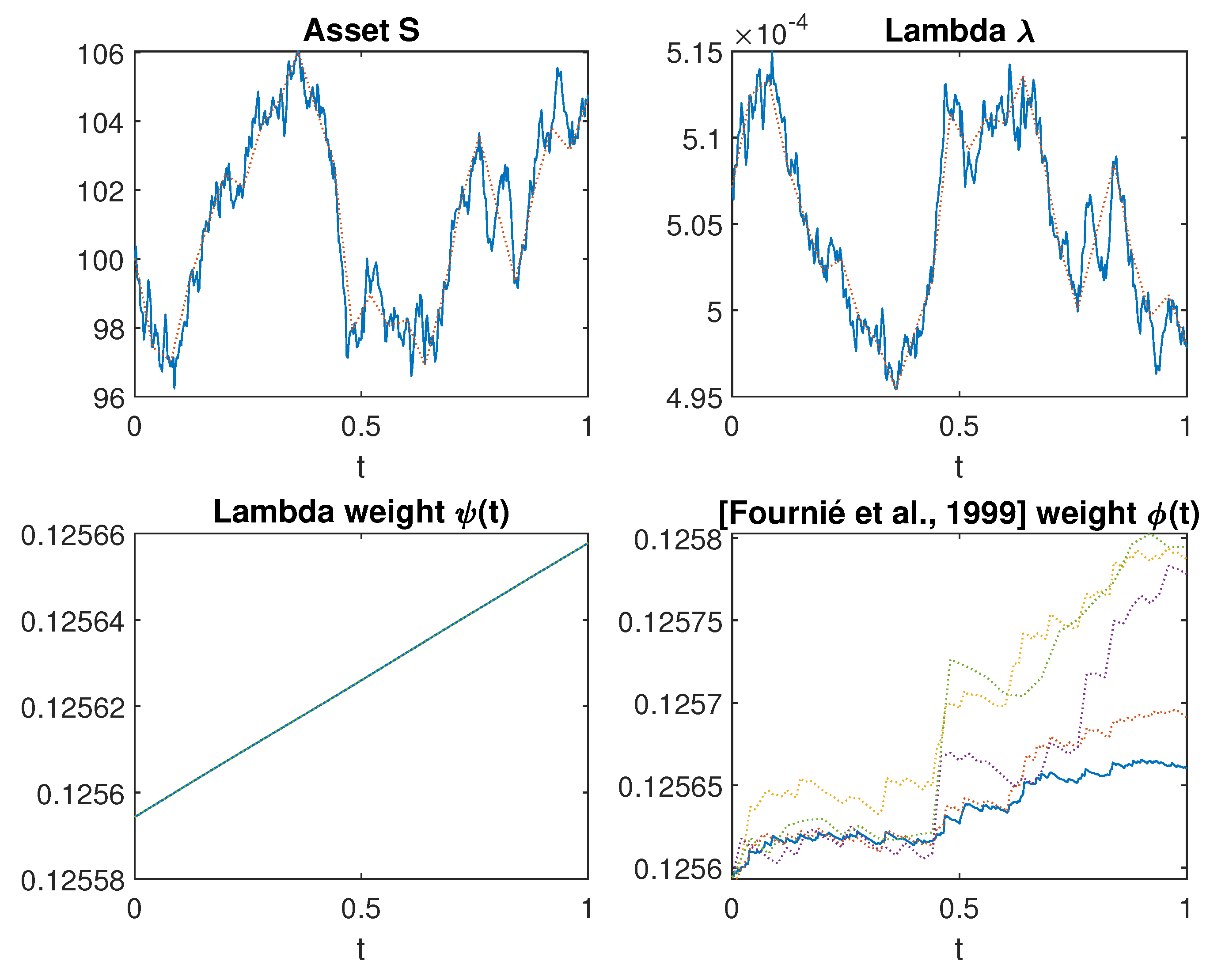
We discretize the interval into subintervals of length with nodes . We generate a discretized Brownian path which is used to compute a reference ("true") trajectory for the processes and . Then, we consider other decomposition of the interval into L subintervals in such a way that the stepsize is an integer multiple of the increment used for computing the Brownian path. This ensures that the set of nodes contains the points at which the convergence of the Euler–Maruyama method is tested. Our choice is to double the discretization step each time by taking , with . The Brownian motion increments on the reference path are aggregated in order to build the increments on the sparse grids that are then used to implement the Euler method. The parameter values are , , , , and .
The upper panels of Figure 1 show the effects of the discretization on the asset price and lambda paths . The blue lines are the reference trajectories on the finer grid, while the red dotted lines are the discrete approximations obtained for . In the lower panels of Figure 1, we plot the corresponding approximated trajectories of the functions and over the discrete grids for . We notice that the function is much affected by the discretization over sparse grids, while is not. Nevertheless, the approximated functions match the reference ones computed on the fine grid more closely as decreases. Therefore, convergence seems to take place. Finally, we remark that the stochastic function seems to be much regular. Indeed, this is in complete agreement with Equation (8), which proves the differentiability with respect to time of the rescaled variation, while the differentiability of function is not so visually evident.
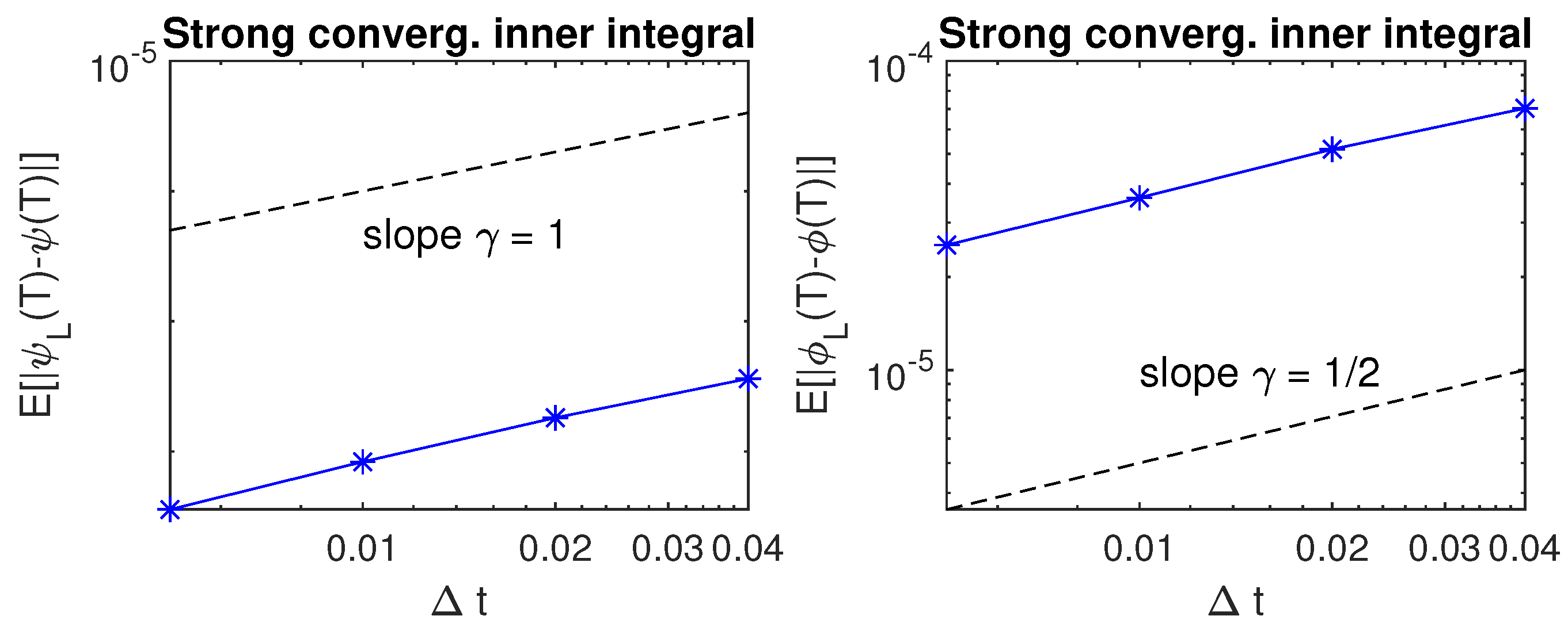
In order to test the strong convergence of the two different methods, we compute , where z is the reference rescaled variation computed by (17) or by (18) on the fine grid and its discrete approximation. A method is said to have strong order of convergence equal to if there exists a constant C such that
for any fixed and sufficiently small. It is well known that the Euler method of integration is of order for Itô stochastic integrals, while it is of order for ordinary differential equations. This marks a departure between the stochastic and the deterministic settings and can support and motivate our approach of computing the rescaled variation by the Riemann integral (18) instead of the Itô integral (17). In our numerical tests, we focus on the error at the endpoint and we test whether the bound holds for some . We compute different Brownian paths over with and then we apply the Euler–Maruyama method with different stepsizes , with . If the condition (19) holds with approximate equality, then we get
namely plotting the approximated errors against on a log–log scale would produce a line with slope .
In Figure 2, the blue asterisk line plots our simulated results. For reference, a dashed line of slope is plotted as well. In both cases the error reduces as becomes smaller but in the case of the lambda approach the slope is 1, suggesting a strong order of convergence of 1, while in the other case the convergence rate is .
We can analyze this further by testing a power law relation or, equivalently, . A least squares fit for and is computed producing the values 1.2945 and 0.4849 for in the two cases, respectively.
Now we come to examine the convergence of the approximation to the weight computed in the two alternative forms
and
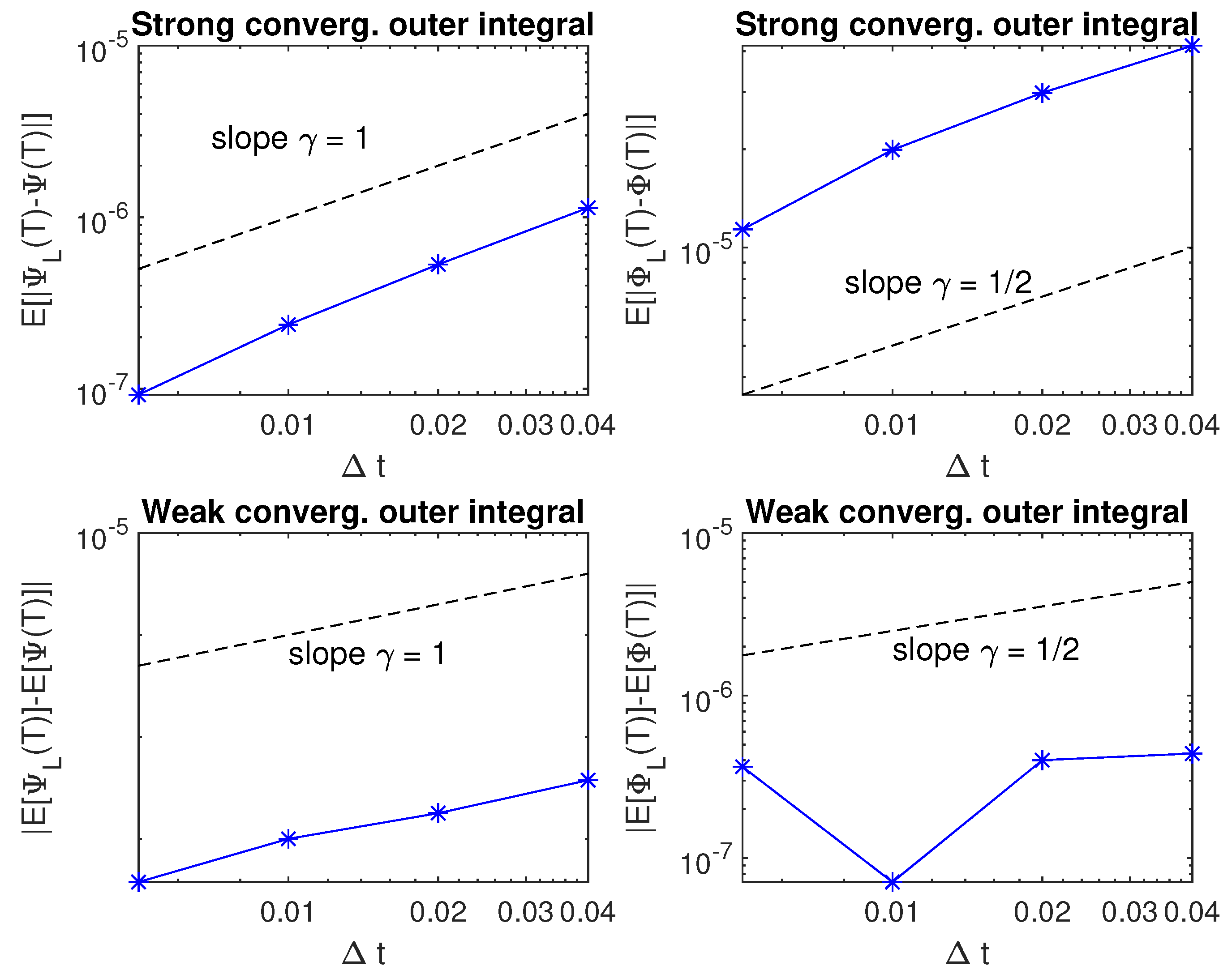
As before, we compute the mean of the error of the approximated integral as becomes small. In the upper panels of Figure 3 we can see that again the error reduces with but, while exhibits a strong order of convergence equal to 1/2, the approximation of still retains a strong order of convergence equal to 1. More precisely, the least squares fit for produces the values 1.2025 and 0.6196 for the strong convergence regression.
This different behavior of the two methods has important consequences even on the weak order of convergence of the integral. This is a less demanding alternative to strong convergence which measures the rate of decay of the error of the means . This error is plotted against on a log–log scale in the lower panels of Figure 3. As expected, the approximation of exhibits a weak order of convergence typical of the Euler–Maruyama method, while in the case of the convergence rate is not much clearer. The least squares fit for produces the values 1.0802 and 0.3307 for the weak convergence regression with the two different methods, respectively. However, the least squares residual for is 1.4119 and does not support a clear order of weak convergence for a double stochastic integral approach.
3.2. Efficiency of the Method
In order to asses the efficiency of our method, we compute the in the case of a Black–Scholes and of a CEV underlying diffusion for the following payoffs:
- European Call/Put option: , ;
- Digital Call/Put option: ,
using the -method, the method proposed by Fournié et al. (1999) and the Monte Carlo finite difference method. The results are displayed in Table 1, Table 2, Table 3 and Table 4. ”Analytic” denotes the closed form solution.
First, let us consider the Black–Sholes framework. In this case, the -method and the method of Fournié et al. (1999) are the same. However we implement the formula (11) for the in two different ways, either by computing the expectation in the right hand side as in Fournié et al. (1999) or by simulating trajectories of the Brownian motion to compute the integral in the left hand side (-method).
From Table 1, we notice that the -method generally outperforms the method of Fournié et al. (1999) as well as the Monte Carlo finite difference method for small number of iterations N, i.e., the -method exhibits a faster convergence speed. The perturbation of the initial condition in the Monte Carlo approach is set to . The Monte Carlo finite difference method performs quite poorly for Digital options, while the -method gives very good results.
When increasing the number of iterations, the results provided by the three methods are more comparable and almost equivalent as shown in Table 2 and Table 3.
Finally, we consider the case of the CEV model. In this case the -method consists in computing the expectation in (15), where the function is given by (16), while the Fournié et al. (1999) method is based on the computation of the expectation in (14). The Monte Carlo finite difference method is implemented with common random numbers. The initial perturbation is set to and in the case of digital options a second order different quotient is used to approximate the delta. The Analytic delta value is computed in terms of the noncentral chi-square distribution—see Hull (2018).
As can be seen from Table 4, the results provided by the -method and the method of Fournié et al. (1999) are almost undistinguishable, while the Monte Carlo finite difference method performs slightly better in the European case but is completely unreliable for binary options with a 20% relative error on the Delta value.
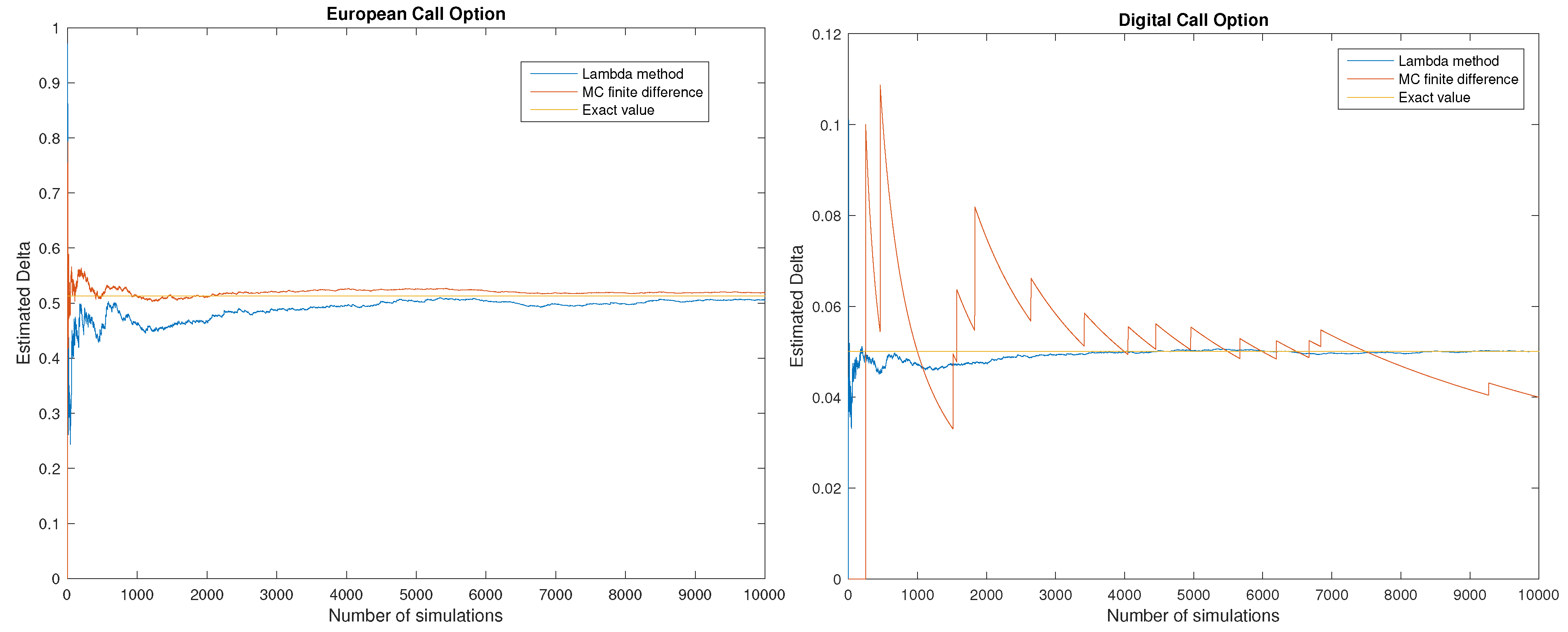
Figure 4 shows the performance of the -method versus the Monte Carlo finite difference for increasing values of the number of simulations N used to compute the expectation. In the case of the European option the Monte Carlo method provides slightly less biased results. This is a well understood phenomenon and a possible way to fix this problem is to localize the integration by parts around the strike price K, as suggested by Fournié et al. (1999). In contrast, for the Digital option case the -method is very efficient, while the Monte Carlo finite difference methods gives very poor results.
4. Greek Estimation from Observed Underlying Prices. An Empirical Case Study
In order to illustrate the model-free nature of our approach in the context of the Malliavin weight method, we consider a case study based on 5-minute observations (open prices) of the EUR/USD exchange rate on the period from 29 February 2016 to 3 June 2016. We propose a nonparametric estimation procedure for computing the Delta of exchange rate options. Prices of derivative securities depend crucially on the form of the volatility of the underlying process, therefore we work in the framework of local volatility models but leave the volatility function unrestricted and estimate it nonparametrically from the observed prices.
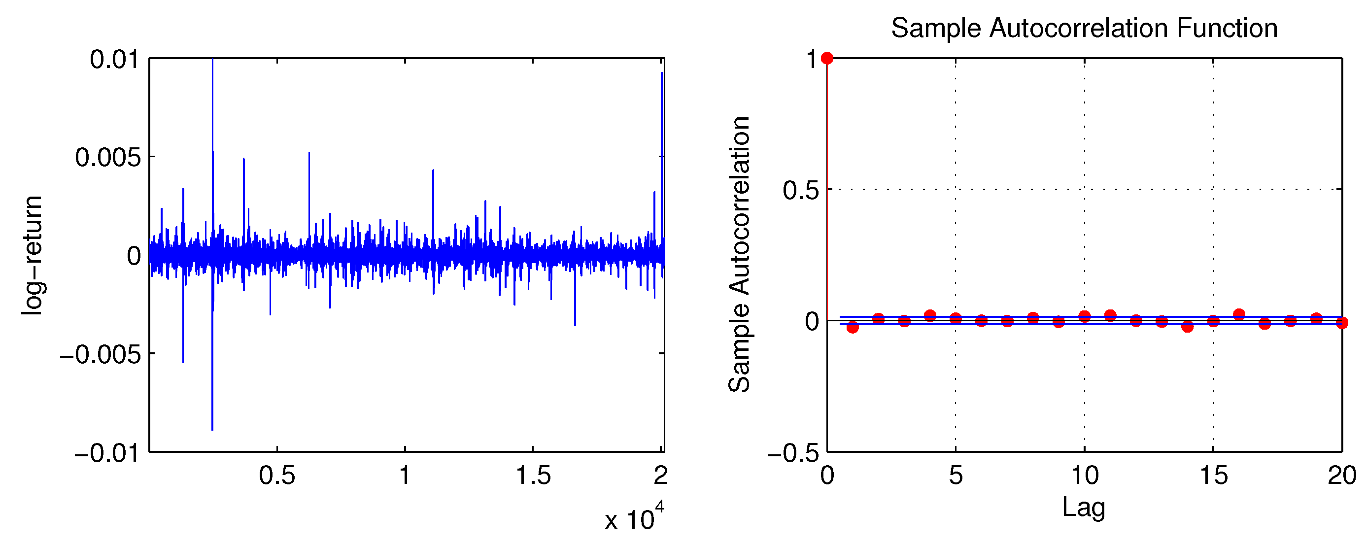
Our sample contains 20,136 observations. Table 5 describes the main features of our data set. Intra-day returns may be contaminated by transaction costs, bid-and-ask bounce effects, etc., leading to biases in the variance measures. A preliminary analysis through the autocorrelation function plot of the 5-min returns is conducted in Figure 5 to detect the presence of market microstructure noise. The degree of first order autocorrelation of log-returns seems very weak, meaning that microstructure effects are not relevant in this sample. However, the autocorrelations decay slowly. To test for stationarity, we performed an augmented Dickey–Fuller nonstationarity test. The nonstationarity hypothesis is rejected at the 90% level. The test is known to have low power, so even a slight rejection means that stationarity of the series is likely.
We assume the risk neutral dynamics for the spot exchange rates S is
Then, the logarithm follows a time-homogeneous Itô diffusion process represented by the following stochastic differential equation
with initial condition , where is a standard real Brownian motion and the real function is such that a single solution of the stochastic differential Equation (23) exists. We remark that we are making no assumptions on the functional form of . Our specific problem is to estimate the diffusion term when we observe a discrete realization of the process via observations , …, at times in the interval and then to price derivatives in the context of the Malliavin weight method.
FIRST STEP: We estimate the diffusion term by means of classical Nadaraya–Watson type estimators of the kind
where is a consistent estimator of the spot volatility at time .
Following Kenmoe and Sanfelici (2014), our choice for is based on the Fourier-Malliavin estimator of the spot volatility. The spot volatility at time is estimated at the opening of each day using the whole high-frequency exchange rate time series
where the k-th Fourier coefficient of the variance process is obtained by Bohr-convolution
from the discrete Fourier transform .
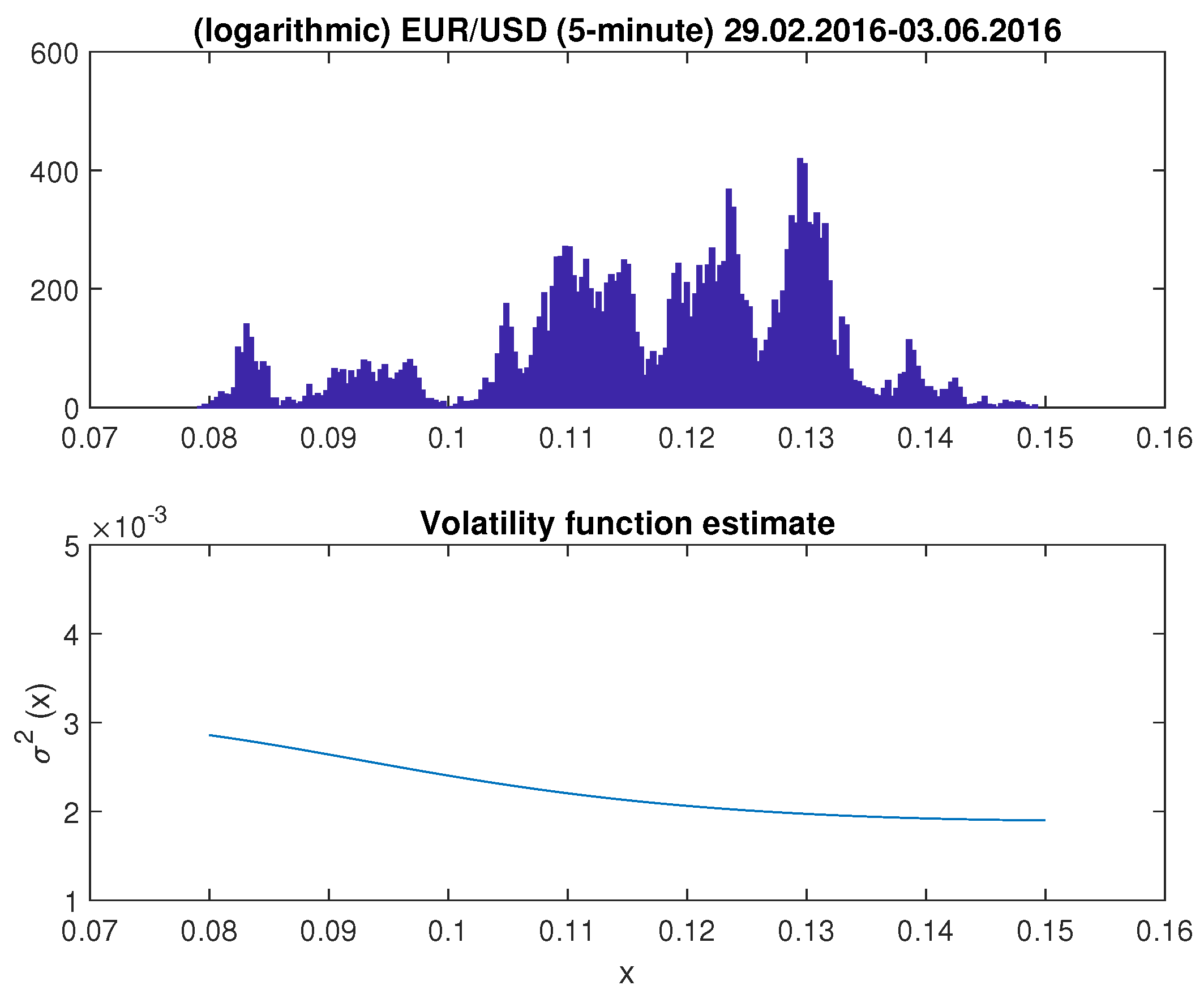
Figure 6 plots the histogram of the distribution of the EUR/USD exchange rate and the nonparametric estimate of the diffusion function of the exchange rate model obtained by the estimator (24). The function is plotted on a uniform grid in the interval . The diffusion function does not look flat or linear, rather it shows the shape of a "smile" with higher volatilities for low exchange rates.
SECOND STEP: The estimated volatility function is then used to generate N realizations of the process (22) and to price a given contingent claim in a Monte Carlo simulation. We generate 100 trajectories by dividing the interval into subintervals and by discretizing the estimated diffusion process by first order Euler method.
THIRD STEP: For each generated trajectory, we estimate the spot functions , and using the Fourier estimation metho— see Mancino et al. (2017)— and we compute the feedback rate function by (A6) in Remark A1:
We remark that each time the Fourier cross-volatility estimation procedure is reiterated the resolution at which the estimated function can be observed becomes lower and lower. To maintain a good resolution, we can exploit the fact that, in the trajectories simulation process, the spot volatility is actually known. Therefore, we can easily compute its discrete Fourier coefficients by
From and , the functions , and can be estimated by the Fourier methodology according to Theorem A2.4
Furthermore, we highlight that any other approach for computing the Malliavin weight is not possible in this context because the computation of the variation process from (6) requires the knowledge of the functional form of the volatility function to perform differentiation.
FOURTH STEP: We compute
via Monte Carlo method, by averaging the argument of the expectation over the simulated sample paths.
As a benchmark for our computations, we solved the associated generalized Black–Scholes equation
with the final condition by (backward Euler) finite difference method. Following Tavella and Randall (2000), we impose linearity conditions on the boundary of a truncated computational domain.
The option delta values are also compared to those obtained by Monte Carlo finite difference and by the Black–Scholes formula with volatility parameter set equal to .
In Table 6, we show the results obtained for the pricing of an European Put option with strike and expiry time year. For simplicity, the risk free interest rate is taken to be . The perturbation of the initial datum in the Monte Carlo finite difference method is set to 0.001.
We notice that the lambda method outperforms the Monte Carlo finite difference method for at-the-money options, due to the lack of regularity of the payoff function f at . However, the Monte Carlo finite difference method works better for out-of-the-money and deep out-of-the-money options and has in general a much smaller variability.
5. Conclusions
We have proposed a possible way to compute the hedging Delta using the Malliavin weight method of Fournié et al. (1999) in a local volatility framework. The advantage of our -method are twofold: on the one hand the advantage is computational, because it allows us to compute the Malliavin weight by a single stochastic integral versus a double stochastic integral as in Fournié et al. (1999). This yields a faster convergence rate in a Monte Carlo experiment, especially for discontinuous payoffs. On the other hand, our approach is nonparametric, as we only assume a general local volatility model and we can estimate the volatility and the other processes involved in the Greek formula with quantities that can be nonparametrically obtained from observed prices.
Author Contributions
Conceptualization, M.E.M. and S.S.; methodology, M.E.M. and S.S.; software, M.E.M. and S.S.; validation, M.E.M. and S.S.; formal analysis, M.E.M. and S.S.; investigation, M.E.M. and S.S.; resources, M.E.M. and S.S.; data curation, M.E.M. and S.S.; writing—original draft preparation, M.E.M. and S.S.; writing—review and editing, M.E.M. and S.S.; visualization, M.E.M. and S.S.; supervision, M.E.M. and S.S.; project administration, M.E.M. and S.S.; funding acquisition, M.E.M. and S.S. All authors have read and agreed to the published version of the manuscript.
Funding
This research received no external funding.
Conflicts of Interest
The authors declare no conflict of interest.
Appendix A
This Section resumes the mathematical computation of the function. The proof of the Theorems A1 and A2 can be found in Malliavin and Thalmaier (2006).
Theorem A1.
Assume that the asset price evolves according to the SDE
with initial value , where a and b are smooth functions. Consider the associated variation process
Then, the rescaled variation defined by
is differentiable with respect to t and it holds that
where
Theorem A2.
Denoting by the quadratic (co-)variation operation, define the following cross-volatilities:
then the function in (A3) has the following expression
References
- Aït-Sahalia, Yacine. 1996. Nonparametric Pricing of Interest Rate Derivative Securities. Econometrica 64: 527–60. [Google Scholar] [CrossRef] [Green Version]
- Barucci, Emilio, Paul Malliavin, Maria Elvira Mancino, Roberto Renò, and Anton Thalmaier. 2003. The price-volatility feedback rate: An implementable mathematical indicator of market stability. Mathematical Finance 13: 17–35. [Google Scholar] [CrossRef] [Green Version]
- Benhamou, Eric. 2003. Optimal Malliavin Weighting Function for the Computation of the Greeks. Mathematical Finance 13: 37–53. [Google Scholar] [CrossRef]
- Bouleau, Nicolas. 2003. Error calculus and path Sensitivity in Financial Models. Mathematical Finance 13: 115–34. [Google Scholar] [CrossRef] [Green Version]
- Cox, J., and S. Ross. 1976. The valuation of options for alternative stochastic processes. Journal of Financial Economics 3: 407–32. [Google Scholar] [CrossRef]
- Davydov, D., and V. Linetsky. 2001. Pricing and Hedging Path-Dependent Options Under the CEV Process. Management Science 47: 949–65. [Google Scholar] [CrossRef] [Green Version]
- Derman, E., and I. Kani. 1994. Riding on the Smile. RISK 7: 32–39. [Google Scholar]
- Dupire, B. 1994. Pricing with a smile. RISK 7: 18–20. [Google Scholar]
- Elie, R., J.-D. Fermian, and N. Touzi. 2007. Kernel estimation of Greek weights by parameter randomization. The Annals of Applied Probability 17: 1399–423. [Google Scholar] [CrossRef] [Green Version]
- Fournié, E., J.M. Lasry, J. Lebuchoux, P.L. Lions, and N. Touzi. 1999. Applications of Malliavin calculus to Monte Carlo methods in finance. Finance and Stochastics 3: 391–412. [Google Scholar] [CrossRef]
- Fournié, E., J.M. Lasry, J. Lebuchoux, and P.L. Lions. 2001. Applications of Malliavin calculus to Monte Carlo methods in finance. II. Finance and Stochastics 5: 201–36. [Google Scholar] [CrossRef]
- Hayashi, T., and P.A. Mykland. 2005. Evaluating hedging errors: An asymptotic approach. Mathematical Finance 15: 309–43. [Google Scholar] [CrossRef]
- Hobson, D., and L. Rigers. 1998. Complete models with stochastic volatility. Mathematical Finance 8: 27–48. [Google Scholar] [CrossRef]
- Hull, J.C. 2018. Options, Futures and Other Derivatives. London: Pearson. [Google Scholar]
- Kenmoe, R., and S. Sanfelici. 2014. An application of nonparametric volatility estimators to option pricing. Decisions in Economics and Finance 37: 393–412. [Google Scholar] [CrossRef]
- Kohatsu-Higa, A., and M. Monteiro. 2001. An Application of Malliavin Calculus to Finance. Available online: https://arxiv.org/pdf/cond-mat/0111563.pdf (accessed on 10 November 2020).
- Malliavin, P. 1997. Stochastic Analysis. A Series of Comprehensive Studies in Mathematics; Berlin/Heildelberg: Springer, vol. 313. [Google Scholar]
- Malliavin, P., and M.E. Mancino. 2002a. Fourier Series method for measurement of Multivariate Volatilities. Finance and Stochastics 6: 49–61. [Google Scholar] [CrossRef]
- Malliavin, P., and M.E. Mancino. 2002b. Instantaneous liquidity rate, its econometric measurement by volatility feedback. Comptes Rendus Mathematique 334: 505–8. [Google Scholar] [CrossRef]
- Malliavin, P., and M.E. Mancino. 2009. A Fourier transform method for nonparametric estimation of volatility. The Annals of Statistics 37: 1983–2010. [Google Scholar] [CrossRef] [Green Version]
- Malliavin, P., and A. Thalmaier. 2006. Stochastic Calculus of Variations in Mathematical Finance. Berlin/Heidelberg: Springer. [Google Scholar]
- Mancino, M.E., M.C. Recchioni, and S. Sanfelici. 2017. Fourier-Malliavin Volatility Estimation: Theory and Practice. Springer Briefs in Quantitative Finance Series; Berlin/Heidelberg: Springer, ISBN 978-3-319-50969-3. [Google Scholar]
- Mancino, M.E., and S. Sanfelici. 2008. Robustness of the Fourier Estimator of Integrated Volatility in Presence of Microstructure Noise. Computational Statistics and Data Analysis 52: 2966–89. [Google Scholar] [CrossRef]
- Mancino, M.E., and S. Sanfelici. 2020. Identifying financial instability conditions using high frequency data. Journal of Economic Interaction and Coordination 15: 221–42. [Google Scholar] [CrossRef]
- Tavella, D., and C. Randall. 1998. Pricing Financial Instruments. The Finite Difference Method. Hoboken: John Wiley & Sons, Inc. [Google Scholar]
| 1. | We emphasize the dependence on the Brownian path, using the subindex W. |
| 2. | The prime stands here for the first derivative with respect to the level . |
| 3. | It should be noticed that the last integral in (7) is a Skohorod integral, for the duality formula with the Malliavin derivative operator . However, if the integrand is adapted to the filtration, then the Skohorod integral and the Itô integral coincide. |
| 4. | In particular, as discussed in Mancino and Sanfelici (2008), the cutting frequencies for the functions and can be taken as and , respectively. Finally, the feedback rate function can be estimated at distinct points in the interval by taking in the Fourier expansion for . Being , this procedure allows for a reconstruction of the feedback rate function at 125 nodes in the interval . |
Figure 1.
Constant Elasticity of Variance model. Parameter values: , , , , , .

Figure 2.
Constant Elasticity of Variance model. Parameter values: , , , , , .

Figure 3.
Constant Elasticity of Variance model. Parameter values: , , , , , .

Figure 4.
Constant Elasticity of Variance model. Parameter values: , , , , , , , .

Figure 5.
Time plot of the 5-min log-returns and ACF for EUR/USD exchange rate on the period from 29 February 2016 to 3 June 2016.
Figure 5.
Time plot of the 5-min log-returns and ACF for EUR/USD exchange rate on the period from 29 February 2016 to 3 June 2016.

Figure 6.
Histogram of the distribution of the logarithmic EUR/USD exchange rate on the period from 29 February 2016 to 3 June 2016 and nonparametric estimation of the diffusion function.
Figure 6.
Histogram of the distribution of the logarithmic EUR/USD exchange rate on the period from 29 February 2016 to 3 June 2016 and nonparametric estimation of the diffusion function.


Table 1.
Black–Scholes model. Parameter values: , , , , .
| Option | N | n | λ-Method | Fournié et al. (1999) | MC Fin. Diff. | Analytic |
|---|---|---|---|---|---|---|
| EC | 1000 | 200 | 0.620603 | 0.584784 | 0.620490 | 0.636831 |
| EP | 1000 | 200 | −0.382432 | −0.409168 | −0.378079 | −0.363169 |
| DC | 1000 | 200 | 0.018054 | 0.017937 | 0.190246 | 0.018762 |
| DP | 1000 | 200 | −0.019501 | −0.020261 | −0.190246 | −0.018762 |
Table 2.
Black–Scholes model. Parameter values: , , , , .
| Option | N | n | λ-Method | Fournié et al. (1999) | MC Fin. Diff. | Analytic |
|---|---|---|---|---|---|---|
| EC | 5000 | 200 | 0.641900 | 0.646569 | 0.633642 | 0.636831 |
| EP | 5000 | 200 | −0.355614 | −0.368940 | −0.364584 | −0.363169 |
| DC | 5000 | 200 | 0.018898 | 0.018950 | 0.019025 | 0.018762 |
| DP | 5000 | 200 | −0.018348 | −0.018951 | −0.019025 | −0.018762 |
Table 3.
Black–Scholes model. Parameter values: , , , , .
| Option | N | n | λ-Method | Fournié et al. (1999) | MC Fin. Diff. | Analytic |
|---|---|---|---|---|---|---|
| EC | 10,000 | 200 | 0.642683 | 0.634604 | 0.633323 | 0.636831 |
| EP | 10,000 | 200 | −0.351281 | −0.359368 | −0.364866 | −0.363169 |
| DC | 10,000 | 200 | 0.018758 | 0.018717 | 0.019025 | 0.018762 |
| DP | 10,000 | 200 | −0.018252 | −0.018755 | −0.019025 | −0.018762 |
Table 4.
Constant Elasticity of Variance model. Parameter values: , , , , , , , .
| Option | λ-Method | Fournié et al. (1999) | MC Fin. Diff. | Analytic |
|---|---|---|---|---|
| EC | 0.0.506340 | 0.506337 | 0.519070 | 0.512955 |
| EP | −0.468663 | −0.468662 | −0.481571 | −0.487045 |
| DC | 0.050183 | 0.050182 | 0.040000 | 0.050090 |
| DP | −0.048846 | −0.048846 | −0.040000 | −0.050090 |
Table 5.
Summary statistics for the sample of the EUR/USD exchange rate on the period from 29 February 2016 to 3 June 2016 (20136 open prices). “Std. Dev.” denotes the sample standard deviation of the variable.
Table 5.
Summary statistics for the sample of the EUR/USD exchange rate on the period from 29 February 2016 to 3 June 2016 (20136 open prices). “Std. Dev.” denotes the sample standard deviation of the variable.
| Variable | Mean | Std. Dev. | Min | Max |
|---|---|---|---|---|
| EUR/USD exchange rate | 1.124517 | 0.015473 | 1.082280 | 1.161020 |
| 5-min log-return (%) | 2.028925 × 10⁻⁴ | 3.302504 × 10⁻² | −8.892366 × 10⁻¹ | 9.972291 × 10⁻¹ |
Table 6.
European put option written on the EUR/USD exchange rate on the period from 29 February 2016 to 3 June 2016.
Table 6.
European put option written on the EUR/USD exchange rate on the period from 29 February 2016 to 3 June 2016.
| Underlying asset value S | 0.9500 | 1.0500 | 1.1000 | 1.1500 | 1.2500 |
| Option delta | |||||
| Lambda method | −0.9892 | −0.9740 | −0.5319 | −0.0938 | 0 |
| Standard deviation | (0.2749) | (0.2021) | (0.0932) | (0.0419) | (0) |
| Monte Carlo finite difference | −0.9899 | −0.7651 | −0.4547 | −0.1590 | −0.0103 |
| Standard deviation | (0.0045) | (0.0045) | (0.0033) | (0.0009) | (0.0004) |
| Finite Difference Method | −0.9974 | −0.8109 | −0.5225 | −0.1774 | −0.0023 |
| Black–Scholes formula | −0.9988 | −0.7957 | −0.4900 | −0.1502 | −0.0021 |
Publisher’s Note: MDPI stays neutral with regard to jurisdictional claims in published maps and institutional affiliations. |
© 2020 by the authors. Licensee MDPI, Basel, Switzerland. This article is an open access article distributed under the terms and conditions of the Creative Commons Attribution (CC BY) license (http://creativecommons.org/licenses/by/4.0/).
Share and Cite
MDPI and ACS Style
Mancino, M.E.; Sanfelici, S. Nonparametric Malliavin–Monte Carlo Computation of Hedging Greeks. Risks 2020, 8, 120. https://0-doi-org.brum.beds.ac.uk/10.3390/risks8040120
AMA Style
Mancino ME, Sanfelici S. Nonparametric Malliavin–Monte Carlo Computation of Hedging Greeks. Risks. 2020; 8(4):120. https://0-doi-org.brum.beds.ac.uk/10.3390/risks8040120
Chicago/Turabian StyleMancino, Maria Elvira, and Simona Sanfelici. 2020. "Nonparametric Malliavin–Monte Carlo Computation of Hedging Greeks" Risks 8, no. 4: 120. https://0-doi-org.brum.beds.ac.uk/10.3390/risks8040120
Note that from the first issue of 2016, this journal uses article numbers instead of page numbers. See further details here.