The Lithium Industry and Analysis of the Beta Term Structure of Oil Companies

Abstract

According to a statement made in the BP Energy Outlook report in 2017, most of the world’s liquid fuel (petroleum) is being consumed by the transportation industry. The mechanisms used to stimulate changes in the energy markets are affected by government policies that act in more ambitious ways than purely market-driven forces; different governments have promoted incentives involving electric mobility, especially in urban areas. The substitution for crude oil by renewable energy inputs in the transport sector is a major concern for oil producers. Among the different types of clean energies, lithium (Li) is currently assuming an increasingly strategic role. The goals of this paper are two-fold: First, we study the dynamics of the lithium industry and then the beta risk behavior of the 10 largest oil companies in the world for the time period between 11 February 2008 and 10 January 2019. We use an approach based on the continuous wavelet transform (CWT) method. The results indicate that there is a period of dependence between late 2013 and 2016 that occurs in the long-run frequencies of between 32 and 198 days for all cases, except for in the case of PetroChina, thereby demonstrating that the beta term is time-varying. We also find evidence that the beta term reflects and advances oil companies’ responsiveness to movements in the lithium market. In the second part of the paper, we study the dynamics of the beta series by using long-run dependence approaches. The results indicate that the betas are highly persistent, with the order of integration found to be significantly above 1 in all cases.

1. Introduction

At the end of the 19th century, there were several engine alternatives competing within the automobile industry. As discussed by Anderson and Anderson (2010), since the late 19th century, all vehicles have been powered by a dominant technology, ranging from steam-powered vehicles to gasoline and electric vehicles. Promoting the use and sources of renewable energy has become the main priority for several countries, with the purpose of achieving a safer and more efficient form of energy consumption linked to economic development that could help alleviate poverty and achieve the environmental objectives embodied in the Paris Agreement, which was ratified by many countries around the world, including 10 OPEC (Organization of the Petroleum Exporting Countries) member countries.

According to the World Oil Outlook (2018), the mechanisms used to stimulate changes in the energy markets are affected by government policies that act in more ambitious ways than purely market-driven forces; different governments have promoted different incentives for electric mobility, especially in urban areas (World Oil Outlook 2017). Among the different types of clean energy production technologies, lithium (Li) is assuming an increasingly strategic role as clean energy technologies emerge. As covered by Jaskula (2019), the use of this essential metal for batteries (56% of the total lithium market) has increased significantly in recent years due to the growing market for electric vehicles and other devices.

The substitution for crude oil by renewable energy inputs in the transport sector is a major concern among oil producers, as most of the global demand for oil comes from this sector. Formative phases of new technologies are already in place. Several researchers and academics, including Bento and Wilson (2016), Sovacool (2016), and Fouquet (2016), have analyzed the formative phases of new technologies, the prospect of a future energy transition, and the associated policy implications, respectively. Schurr and Netschert (1960) were early examiners of developments involving crude oil in transportation and renewable energy, and also of past technology transitions. In the next 10 to 25 years, the use of crude oil, which has long been the main fuel used for transportation, could change due to the increase of renewables being utilized for power generation, leading to oil losing its currently essential role in the energy market and heading toward similar low price levels as coal (for further details regarding this trend, see Cherif et al. 2017).

The previous statement is important because in addition to the energy sector, the transport sector also consumes a large portion of the fuel (petroleum) that comes from crude oil; the global transport sector’s demand for oil has remained at just under 60% of total crude oil demand (see BP Energy Outlook 2017), while the sector produces 70% of total greenhouse gas emissions (IPCC Fourth Assessment Report: Mitigation of Climate Change 2007). On the other hand, electric vehicles (EV), including battery electric vehicles (BEVs), hybrid electric vehicle (HEVs), plug-in hybrid electric vehicles (PHEVs), and fuel cell electric vehicles (FCEVs), are becoming increasingly popular in the transport sector. Hao et al. (2016) state in their research paper that the recent increase in lithium consumption is due to increased global demand for electric vehicles (EV). Randall (2016) states that 35% of the new cars sold in the year 2040 will operate using electrical energy alone, which will cause the next oil crisis. Additionally, the BP Energy Outlook (2020) notes that although the demand for oil in emerging markets is expected to increase until the early 2030s, this demand would not compensate for the decreasing demand that is expected to occur in the developing world (this is expected to be a more than 90% decrease compared to the demand level for the transport industry in 2018) due to the increase in the use of electrification in passenger cars and in light and medium trucks. BP concludes in its outlook report that demand for liquid fuels is being fundamentally undermined by the electrification of transport, thanks in part to the lithium industry, which the authors in this research paper concur with. This is important because the growth in electric car production and the corresponding decrease in the demand for oil for transportation purposes is expected to cause a gradual decrease in total oil demand, which could affect oil prices and the oil industry at large, leading to crude oil losing its role as the world’s main transportation fuel. A consequence of this is that the lithium industry poses risks to the oil industry, or more precisely, the lithium industry contributes to the risk that the oil companies face. Identifying how the dynamics of the lithium industry affect the risk behavior of oil companies is useful for investors who need to know about the relative sensitivities of industry stock returns based on changes in the market.

Miller (1977) argued that the relationship between uncertainty and divergence of opinions about returns on securities and risk go together, justifying the common view that the main differences of opinions are related to the riskiest stocks.1 Similarly, the commodity markets are complex systems where agents interact with different time frequencies to achieve their objectives, although most econometric methods that we can find in the relevant literature are based on frequency and time components separately (see Vacha and Barunik 2012). This paper looks at both of these components together, while noting that the stock market is composed of a diverse group of participants (intraday traders, hedging strategists, portfolio managers, financial and non-financial institutions, etc.) who operate on different time scales, depending upon their varying requirements or preferences. In this context, the variables might change over different time scales, affecting the relationship between them in terms of their dynamic structure.

Following the line of research carried out by Monge and Gil-Alana (2018, 2019) and Gil-Alana and Monge (2019) on the lithium industry, to our knowledge this is the first paper trying to analyze and relate the lithium industry with the beta term structure of oil companies. Our contributions are two-fold. First, we analyze how the interconnections and the dynamic correlations between the lithium industry and the conventional beta term structure of oil companies change across different time horizons2, using methodologies based on Continuous Wavelet Transform (CWT) (see Aguiar-Conraria and Soares 2011a, 2011b; Connor and Rossiter (2005); Naccache (2011); Krätschell and Schmidt (2012); Kristoufek et al. (2012a, 2012b, 2013); Vacha and Barunik (2012); Vacha et al. (2013); Abdullah et al. (2016); Filip et al. (2016), among others)3. Using this method, we are able to localize the structural changes over time. The motivation for the study lies in the importance of measuring the dynamic correlations and the anlaysis of the time scale betas, which will allow future research on asset pricing according to the investment horizon and the behavior of said assets depending on the time horizon.

With the results of this analysis, we will focus on the statistical properties, whereby we will use fractional integration techniques to analyze the degree of persistence observed in the series, analyzing the stationary processes related to transitory shocks and permanent shocks (see, Gil-Alana and Hualde 2009; Monge et al. 2017; etc.).

The main results indicate that there is a period of dependence between late 2013 and 2016 that occurs in the long-run frequencies of between 32 and 198 days for all cases, except PetroChina, demonstrating that the beta term is time-varying. We also find evidence that the beta term reflects and advances the oil companies’ responsiveness to movements in the lithium market. In the second part of the paper, we study the dynamics of the beta series by using long-run dependence approaches. The results indicate that the betas are highly persistent, with an order of integration significantly above 1 in all cases.

The rest of the paper is structured as follows. Section 2 comprises the literature review. Section 3 contains a description of the data and presents the methodology used in the paper. In Section 4, we discuss the main empirical results, while conclusions are offered in Section 5.

2. Literature Review

From a theoretical perspective, the capital markets expose investors to market risk. Analyzing these risks is key to investing. The parameter “beta” in the CAPM (Capital Asset Pricing Model) model (Sharpe 1964) plays a central role in modern finance. The only relevant measure of stock risk that explains how investors should act and price risk securities is the “beta” term (Shah et al. 2018). Rua and Nunes (2012) explained that the beta reflects the responsiveness of an asset to movements in the market portfolio, being a linear function of the variability in each stock’s return in certain larger markets.

To study the beta time decomposition, researchers use conventional time scales, such as daily, weekly, monthly, or annual scales. However, when we change the time scale, for example from daily to weekly, the return interval loses information because the number of sample points decreases. Traditionally, it has been assumed that beta is constant though time. Fama and MacBeth (1973) argued that the beta risk is assumed to be a constant using the ordinary least squares (OLS) approach to get the CAPM beta. However, another line of research argues that the beta of a risky asset is time-varying, because the expectations of economic agents for the future returns are random variables (conditional) (see Klemkosky and Martin 1975 and Bollerslev et al. 1988). In the same way, the research by Müller et al. (1997) maintains that multiple layers of investment horizons or time scales (from seconds to years) form the market. Additionally, Shah et al. (2018) criticize the incapability of the CAPM to capture the heterogeneous reality of the real-world markets4. It is not true that all investors experience the same degree of systematic risk as measured by the beta, therefore the CAPM homogeneity assumption would not be fulfilled. Blume (1971, 1975), Fabozzi and Francis (1977, 1978), Sunder (1980), Alexander and Benson (1982), Collins et al. (1987), Harvey (1989, 1991), Ferson and Harvey (1991, 1993), Bollerslev et al. (1988), Fama and French (1997, 2006), Jagannathan and Wang (1996), Ghysels (1998), Reyes (1999), Lettau and Ludvigson (2001), Wang (2003), Lewellen and Nagel (2006), Ang and Chen (2007), and Kim and Kim (2016), among many others, argued that the beta coefficient varies over time. Others researchers found evidence of the use of OLS and the inability to capture the dynamics of the beta (see Harvey 1989; Ferson and Harvey 1991, 1993; Saleem and Vaihekoski 2010). Subsequent investigations concluded that the unconditional CAPM with a constant beta over time does not outperform the conditional CAPM with a variable beta (see Jagannathan and Wang 1996; Lettau and Ludvigson 2001; Beach 2011). On the other hand, the instability of betas over time causes practical problems, such as in the interpretation of betas, which change over time, and in the decision to use CAPM. Related to this, in the literature there is empirical evidence related to equity yields and the temporary structure (see Groenewold and Fraser 1999).

In line with the above, Van Binsbergen et al. (2012) found differences in the risk premiums between short-term and long-term dividends, finding that the slope related to the dividend risk premium was downward. The results obtained by Lettau and Wachter (2011) and Croce et al. (2014) were consistent with this. In the research publication by Van Binsbergen et al. (2013), the authors concluded that the risk premium for a long-maturity dividend fluctuates in periods related to expansion (higher) and recession (lower). The same results were obtained with other international indices (see Van Binsbergen and Koijen 2017). In addition, regarding the volatility of equity yields and expected returns, Campbell and Viceira (2005) stated that the slope trended downward in relation to the horizon. According to McNevin and Nix (2018), reconciling the beta estimate with the facts mentioned above is not straightforward, beacuause the standard market beta should have a complete description and capture time-varying behavior at different frequencies; one must avoid submitting to assumptions involving restrictions on time horizons and frequency changes, since the specific information varies over time.

In the seminal work by Fama and MacBeth published in 1973, it was assumed that the beta risk was constant in the CAPM. Later, other researchers such as Klemkosky and Martin (1975), Bollerslev et al. (1988), and Harvey (1989) demonstrated that the beta of a risky asset should be time-varying due to the conditionality and the variability expectations of economic agents for future returns. More empirical literature on the evidence relating to the variation of the beta terms in equity portfolios was produced by Jagannathan and Wang (1996), Lewellen and Nagel (2006), Bali (2008), and Bali and Engle (2010, 2014).

Bollerslev et al. (1988), Harvey (1989), Jagannathan and Wang (1996), Lewellen and Nagel (2006), Bali (2008), and Bali and Engle (2010, 2014) produced important early studies that found significant time variations in the conditional betas of equity portfolios. The research carried out by Bali et al. (2016) allowed us to understand the sensitivity of an asset in the market portfolio in terms of time-varying and future investment opportunities. González et al. (2018), after analyzing portfolios and the relative weights of the total mixed-frequency conditional betas, reported on the differences over time.

Regarding wavelet analysis, several studies such as Rua and Nunes (2012) used this methodology to analyze the market beta according to the CAPM theory. Yi et al. (2014) used wavelets in financial time series to detect jumps in the high frequency range. The influence during the US subprime crisis of 2007 and in the Islamic and non-Islamic Asian stock markets was investigated by Gallegati (2012) and Saiti et al. (2016). To show how the different investment horizons and the different market participants affect diversifiable risk, Malagon et al. (2015) and Faria and Verona (2018) used wavelet decomposition to forecast stock market returns in different time frequency domains.

Kang et al. (2017) based their research on the wavelets and their explanatory power for different time frequency betas to obtain information about returns and prices. Other authors such as Bansal and Yaron (2004), Bansal et al. (2005), and Parker and Julliard (2005) argued that in certain time frequencies of the standard betas, the relevant information for the pricing of risky assets can be found. Based on this, we expand the previous arguments in this paper and offer another step in the research on equity yields and the beta term structure.

Based on the above, this paper is the first to use the CWT method to calculate the wavelet coherency in order to localize the structural changes over time, using the phase difference in order to understand the synchronism between the lithium industry and changes to the conventional beta values of oil companies. In addition, long-term memory techniques are applied to the betas in order to investigate their degree of dependence over time.

3. Data and Methodology

3.1. Dataset

The choice of oil companies for the dataset was based on the fact that they are among the world’s largest oil firms according to revenue and are listed in the largest stock markets. This criteria ensures that the chosen firms are among the largest players in the market and their stocks are highly liquid. Additionally, we considered only these ten largest oil companies (and no more) because the markets for similar companies (in the case of petroleum) have similar risks.

Further to this criteria, and acording to the classification done by Thomson Reuters in 2019, our final dataset included the world’s ten largest oil companies, namely Sinopec (Pekin, China), Royal Dutch Shell PLC (La Haya, Netherlands), Saudi Aramco (Dhahran, Saudi Arabia), PetroChina Co., Ltd. (Pekin, China), British Petroleum (London, UK), Exxon Mobil (Irving, TX, USA), Total S.A. (Paris, France), Chevron Corp (San Ramon, CA, USA), Rosneft (Moscow, Russia), and Gazprom (Moscow, Russia). We also used the exchange indices to calculate the time series beta5 of each company. In

Table 1. Companies and data information.

Name of the company	Exchange Market	Revenue (in Billion U.S. Dollars)
China Petroleum and Chemical Corp (Sinopec)	Shanghai Stock Exchange	432.54
Royal Dutch Shell PLC	Euronext Amsterdam	382.97
Saudi Aramco	Saudi Arabian Stock Exchange	356.00
PetroChina Co., Ltd.	Shanghai Stock Exchange	347.76
BP PLC	London Stock Exchange	296.97
Exxon Mobil Corp	NYSE Consolidated	275.54
Total SA	Euronext Paris	185.98
Chevron Corp	NYSE Consolidated	157.21
NK Rosneft PAO	Moscow Interbank Currency Exchange (MICEX)	132.73
Gazprom PAO	Moscow Interbank Currency Exchange (MICEX)	129.41

, company data are ordered from highest to lowest in terms of stock market capitalization. The Solactive Global Lithium Index represents the lithium industry. Data were obtained from the Thomson Reuters Eikon database, covering the period ranging from 11 February 2009 to 10 January 2019 and expressed in US dollars. The frequency of the data is daily.

3.2. Methodology

3.2.1. Wavelet Analysis

The wavelet methodology is used to analyze time series in the time frequency domain. Following Crowley (2007), Vacha and Barunik (2012), Aguiar-Conraria and Soares (2011a, 2011b, 2014), Dewandaru et al. (2016), Tiwari et al. (2016), Jammazi et al. (2017), and others, we applied a continuous wavelet transform (CWT) to map one variable as a function of time into two variables as functions of time and frequency. With this transform, we were able to select frequency values and time parameters without losing any information. We used two tools in this paper: the wavelet coherency and wavelet phase difference.

This methodology can be used without the need for the time series to be stationary. Additionally, this methodology is interesting if one wants to find evidence of the potential changes in a time series pattern in the time frequency domain.

A wavelet coherency is a two-dimensional diagram that correlates the time series and identifies hidden patterns or information in the time and frequency domains. The Wavelet Transform, $W{T}_x\left(a,\tau \right)$ of a time series $x\left(t\right)$, which is obtained by using a mother wavelet $\psi$, is defined as:

$$W{T}_x\left(a,\tau \right)={{\displaystyle \int }}_{-\infty }^{+\infty }x\left(t\right)\frac{1}{\sqrt{a}}{\psi }^{*}\left(\frac{t-\tau }{a}\right)dt,$$

(1)

where $W{T}_x\left(a,\tau \right)$ are the wavelet coefficients of $x\left(t\right)$; the position of a wavelet in the frequency domain is defined by a, while τ is the position in the time domain. Therefore, by mapping original series into a function of τ and a, we can obtain information concurrently on the time and frequency. This procedure is called the wavelet transform. The mother wavelet used in this analysis is the Morlet wavelet, because it is a complex sine wave within a Gaussian envelope that allows the synchronism between the time series to be measured (see Aguiar-Conraria and Soares 2014 for the properties of this wavelet).

The wavelet coherence (WCO) helped us to understand the interaction and integration between the two series. The wavelet coherence is defined as:

$$WC{O}_{xy}=\frac{SO\left(W{T}_x\left(a,\tau \right)W{T}_y{\left(a,\tau \right)}^{*}\right)}{\sqrt{SO\left({\left|W{T}_x\left(a,\tau \right)\right|}^2\right)SO\left({\left|W{T}_y\left(a,\tau \right)\right|}^2\right)}},$$

(2)

where SO is a smoothing operator in terms of both time and scale. Without the smoothing operator, the wavelet coherency would always be one for all times and scales (see Aguiar-Conraria and Soares 2014, for details). On Aguiar-Conraria’s website, the Matlab computer programs related to the continuous wavelet transform (CWT) are available.

3.2.2. Fractional Integration

We also use techniques based on long memory and fractional integration. For this purpose, we define an integrated process of order 0 or I(0) as a covariance or second-order stationary process, with the feature that the infinite sum of its autocovariances is finite. Using the frequency domain representation, an I(0) process can be defined as a process with a spectral density function (e.g., the Fourier transform of the autocovariances) that is positive and finite at the smallest (zero) frequency. These are very broad definitions that include not only the white noise model, but also weakly autocorrelated structures such as the one produced by the stationary and invertible autoregressive moving average (ARMA) models. Dealing with the degree of persistence, at the other extreme is a non-stationary processes, defined as having a unit root, also named the integrated order of 1, i.e., I(1) processes, which in their simplest form comprise the random walk model described by:

$$\hspace{0.17em}(1\hspace{0.17em}\hspace{0.17em}\hspace{0.17em}-\hspace{0.17em}\hspace{0.17em}B)\hspace{0.17em}{x}_t\hspace{0.17em}\hspace{0.17em}\hspace{0.17em}\hspace{0.17em}=\hspace{0.17em}\hspace{0.17em}\hspace{0.17em}{u}_t\hspace{0.17em},\hspace{0.17em}\hspace{0.17em}\hspace{0.17em}\hspace{0.17em}\hspace{0.17em}\hspace{0.17em}\hspace{0.17em}\hspace{0.17em}\hspace{0.17em}\hspace{0.17em}\hspace{0.17em}\hspace{0.17em}\hspace{0.17em}\hspace{0.17em}\hspace{0.17em}\hspace{0.17em}\hspace{0.17em}\hspace{0.17em}\hspace{0.17em}\hspace{0.17em}t\hspace{0.17em}\hspace{0.17em}\hspace{0.17em}\hspace{0.17em}=\hspace{0.17em}\hspace{0.17em}\hspace{0.17em}\hspace{0.17em}1\hspace{0.17em},\hspace{0.17em}2\hspace{0.17em},\hspace{0.17em}\hspace{0.17em}\dots \hspace{0.17em},\hspace{0.17em}\hspace{0.17em}\hspace{0.17em}\hspace{0.17em}\hspace{0.17em}$$

(3)

where B is the backshift operator (Bx_t = x_t−1) and u_t is I(0). Note that if u_t is an ARMA(p, q) process, x_t is then an autoregressive integrated moving average (ARIMA (p, 1, q)) process. However, these two structures, the stationary I(0) and the non-stationary I(1), can be included in a more flexible specification known as the fractionally integrated moving average or I(d), where d can be any real value. Thus, extending Equation (3) to the fractional case:

$$\hspace{0.17em}{(1\hspace{0.17em}\hspace{0.17em}\hspace{0.17em}-\hspace{0.17em}\hspace{0.17em}B)}^d\hspace{0.17em}{x}_t\hspace{0.17em}\hspace{0.17em}\hspace{0.17em}\hspace{0.17em}=\hspace{0.17em}\hspace{0.17em}\hspace{0.17em}{u}_t\hspace{0.17em},\hspace{0.17em}\hspace{0.17em}\hspace{0.17em}\hspace{0.17em}\hspace{0.17em}\hspace{0.17em}\hspace{0.17em}\hspace{0.17em}\hspace{0.17em}\hspace{0.17em}\hspace{0.17em}\hspace{0.17em}\hspace{0.17em}\hspace{0.17em}\hspace{0.17em}\hspace{0.17em}\hspace{0.17em}\hspace{0.17em}\hspace{0.17em}\hspace{0.17em}t\hspace{0.17em}\hspace{0.17em}\hspace{0.17em}\hspace{0.17em}=\hspace{0.17em}\hspace{0.17em}\hspace{0.17em}\hspace{0.17em}1\hspace{0.17em},\hspace{0.17em}2\hspace{0.17em},\hspace{0.17em}\hspace{0.17em}\dots \hspace{0.17em},\hspace{0.17em}\hspace{0.17em}\hspace{0.17em}\hspace{0.17em}\hspace{0.17em}$$

(4)

where u_t is I(0) and d can be a fractional value. In this context, if d = 0, x_t is I(0) or is the short-term memory case, as opposed to the long-term memory case if d > 0. If this is in the range of (0, 0.5) then this represents long-term memory, although still of the second stationary order, while if d belongs to [0.5 1) then this represents long-term memory that is non-stationary but mean-reverting, with shocks having long-lasting effects and disappearing very slowly. If d = 1, x_t is I(1) and d is also above 1. In the last two cases, the series do not revert to the mean.6

Processes such as (4) where d > 0 belong to the long-term memory category, meaning that the observations are strongly dependent even if they are far apart in time. The I(d) models with fractional values of d became popular in the 1990s in the works by Sowell (1992), Beran (1994), Baillie (1996), Gil-Alana and Robinson (1997), Ellis (1999), and others. They have also been employed more recently in the analysis of various metals and products by authors such as Panas (2001), Arouri et al. (2012), Gil-Alana and Tripathy (2014), and Gil-Alana et al. (2015), among many others.

We estimate the differences in parameter d by using a parametric method that approximates the likelihood function throughout the Whittle function in the frequency domain, as proposed in Dahlhaus (1989), which we implement through a simple version of the tests performed Robinson (1994), which are widely used in empirical applications.

4. Empirical Results

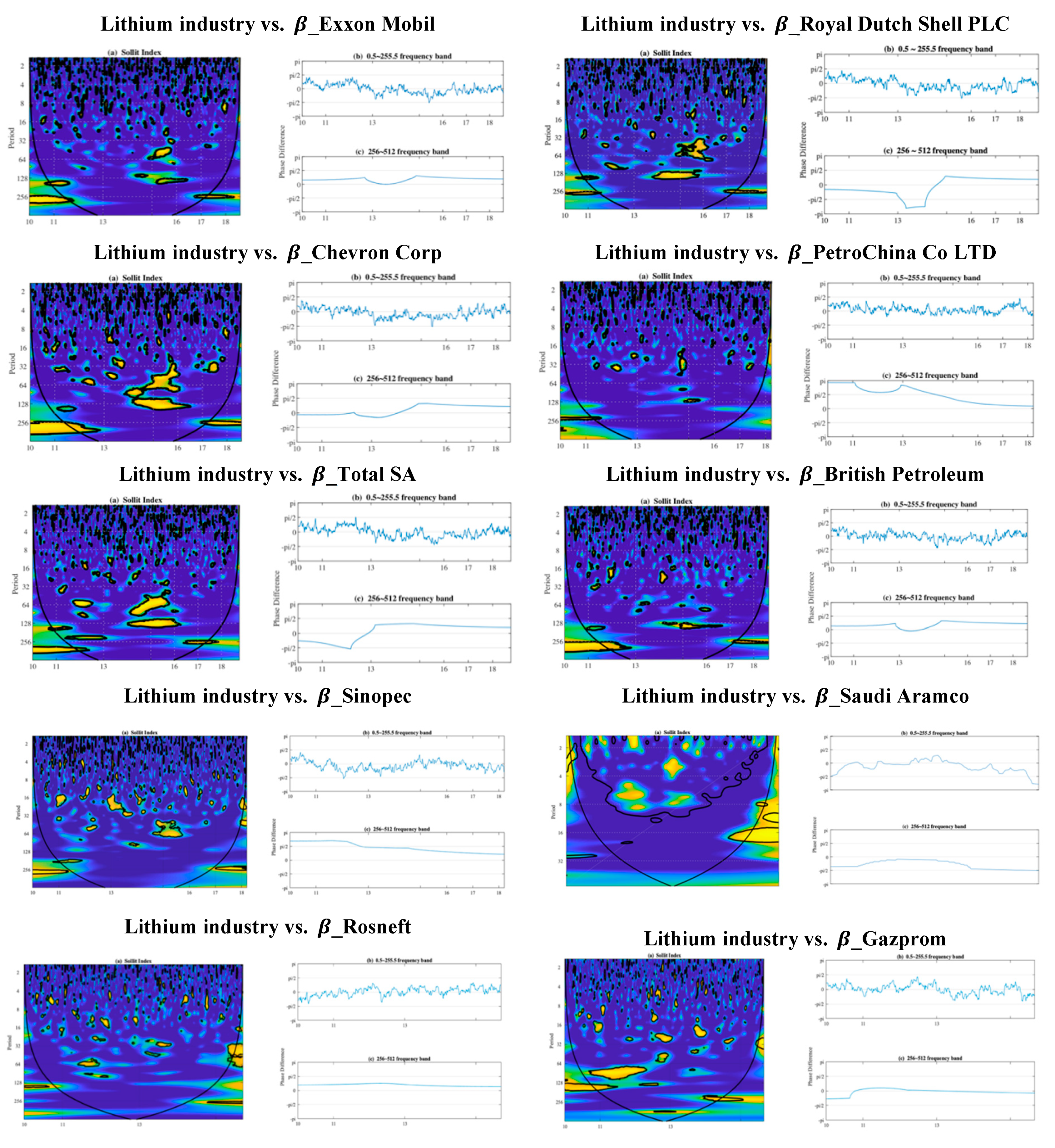
The first part of this section focuses on the wavelet analysis. Figure 1 represents the wavelet coherency and the phase difference between the beta of each oil company and the lithium industry, showing evidence of varying dependence between both time series across different frequencies and over time.

In the panels on the left side of Figure 1, we display the wavelet coherency values to estimate how the lithium industry affects the behavior of the beta of each oil company at different frequencies and how these values evolve over time. Additionally, with this methodology we are able to see the possible presence of structural changes.

Figure 1 tells us when (time is shown in the horizontal axis, from the beginning to the end of the sample period) and at which frequencies (these are shown on the vertical axis, from scale 1 (a single day) up to scale 512 (approximately two market years7)) the interrelations occur and when they are the strongest. First, we calculated the wavelet coherency, showing that the main regions with statistically significant coherency are located at low frequencies (corresponding to cycles between 32 to 198 days, where the regions show statistically significant coherence). The most important ones start around 2013, telling us how important and strong the relation is between the time series (high levels of dependence). In the case of PetroChina, there is no evidence of dependence. For the Russian oil companies (e.g., Gazprom), dependence starts in late 2010, reaching high levels of dependence centered over the long term (lower frequencies) in the year 2016.

Secondly, we founf the partial phase difference, giving us information about the magnitude of the impact that a shock in one variable has on another. For the cases mentioned before, and looking at the 5% significance level, the phase differences are between 0 and −π/2. This means that at this frequency, there is a negative correlation between the lithium industry and the non-diversifiable risk related to the analyzed oil companies. Economically, this means that the lithium industry lags behind the beta of the oil companies, resulting in the ß term reflecting and advancing the responsiveness of the oil companies to movements in the lithium market.

In accordance with Candelon et al. (2008), we also demonstrate with this result that the beta of the oil companies is time-varying, depending on whether this is assessed in the short or long term (higher and lower frequencies, respectively).

Next, we move to the long-term memory analysis. Across

Table 2. Estimates of d for the betas with white noise.

	No Regressors	An Intercept	A Linear Time Trend
Exxon	1.00	1.11	1.11
	(0.97, 1.03)	(1.08, 1.14)	(1.08, 1.14)
Royal Dutch Shell	1.00	1.12	1.12
	(0.97, 1.03)	(1.10, 1.15)	(1.09, 1.15)
Chevron	1.00	1.09	1.09
	(0.97, 1.03)	(1.07, 1.12)	(1.07, 1.12)
PetroChina	0.98	1.09	1.09
	(0.95, 1.00)	(1.06, 1.13)	(1.06, 1.13)
Total SA	1.00	1.10	1.10
	(0.97, 1.03)	(1.08, 1.13)	(1.08, 1.13)
British Petroleum	1.00	1.15	1.15
	(0.96, 1.03)	(1.11, 1.18)	(1.11, 1.18)
Sinopec	1.04	1.05	1.06
	(0.99, 1.08)	(0.99, 1.10)	(1.00, 1.10)
Saudi Aramco	0.94	1.08	1.08
	(0.85, 1.04)	(0.92, 1.24)	(0.91, 1.24)
Rosneft	0.93	0.83	0.87
	(0.85, 1.01)	(0.77, 0.99)	(0.76, 1.00)
Gazprom	0.96	0.92	0.92
	(0.93, 1.03)	(0.86, 1.01)	(0.86, 1.01)

Note: The values in parentheses indicate the 95% confidence band for the values of d; those in bold indicate the selected model for each series.

,

Table 3. Estimated coefficients for the selected models in Table 2 with white noise.

	No Regressors	An Intercept	A Linear Time Trend
Exxon	1.11	0.98911	0.000007
	(1.08, 1.14)	(10,829.35)	(1.74)
Royal D.	1.12	0.94053	0.000028
	(1.09, 1.15)	(5586.11)	(3.21)
Chevron	1.09	1.007611	−0.000006
	(1.07, 1.12)	(10,981.33)	(−1.72)
PetroChina	1.09	0.989113	0.000007
	(1.06, 1.13)	(10,829.33)	(1.64)
Total SA	1.10	1.00405	---
	(1.08, 1.13)	(9699.80)
BP PLC	1.15	0.75244	0.000111
	(1.11, 1.18)	(1370.34)	(3.08)
Sinopec	1.05	0.9863	---
	(0.99, 1.10)	(226.50)
Saudi Aramco	1.08	1.1847	---
	(0.92, 1.24)	(12.47)
NK Rosneft PAO	0.87	0.5582	−0.00023
	(0.76, 1.00)	(74.55)	(−2.30)
Gazprom PAO	0.92	0.5289	−0.00034
	(0.86, 1.01)	(49.03)	(−4.50)

,

Table 4. Estimates of d for the betas with autocorrelateion.

	No Regressors	An Intercept	A Linear Time Trend
Exxon	0.99	1.17	1.17
	(0.95, 1.05)	(1.13, 1.21)	(1.13, 1.21)
Royal D.	0.99	1.17	1.17
	(0.95, 1.05)	(1.14, 1.21)	(1.14, 1.21)
Chevron	0.99	1.12	1.12
	(0.95, 1.05)	(1.09, 1.16)	(1.09, 1.16)
PetroChina	0.99	1.07	1.07
	(0.95, 1.05)	(1.03, 1.11)	(1.03, 1.11)
Total SA	0.99	1.22	1.22
	(0.94, 1.05)	(1.18, 1.27)	(1.18, 1.27)
BP PLC	0.99	1.07	1.07
	(0.95, 1.05)	(1.03, 1.12)	(1.03, 1.12)
Sinopec	0.89	0.92	0.91
	(0.79, 1.01)	(0.87, 1.03)	(0.87, 1.03)
Saudi Aramco	0.89	1.04	1.05
	(0.80, 1.02)	(0.93, 1.12)	(0.93, 1.13)
NK Rosneft PAO	0.87	0.98	0.97
	(0.94, 1.02)	(0.91, 1.09)	(0.91, 1.07)
Gazprom PAO	0.93	0.93	0.92
	(0.88, 1.02)	(0.88, 1.01)	(0.88, 1.02)

Note: The values in parentheses indicate the 95% confidence band for the values of d; those in bold indicate the selected model for each series.

and

Table 5. Estimated coefficients for the selected models in Table 4 with autocorrelation.

	No Regressors	An Intercept	A Linear Time Trend
Exxon	1.17	0.98911	0.000013
	(1.13, 1.21)	(10,962.08)	(1.93)
Royal D.	1.17	0.94053	0.000034
	(1.14, 1.21)	(5648.58)	(2.71)
Chevron	1.12	1.007611	−0.0000085
	(1.09, 1.16)	(11,050.48)	(−1.75)
PetroChina	1.07	1.182063	---
	(1.03, 1.11)	(398.55)
Total SA	1.22	1.00402	---
	(1.18, 1.27)	(9996.64)
BP PLC	1.07	0.75248	0.000113
	(1.03, 1.12)	(1375.82)	(5.48)
Sinopec	0.92	0.9865	---
	(0.87, 1.03)	(433.20)
Saudi Aramco	1.04	1.1856	---
	(0.93, 1.12)	(13.18)
NK Rosneft PAO	0.97	0.5269	−0.00047
	(0.91, 1.07)	(47.47)	(−1.83)
Gazprom PAO	0.92	0.5581	−0.00024
	(0.88, 1.02)	(74.21)	(−1.96)

Note: The values in parentheses indicate the 95% confidence band for the values of d; those in bold indicate the selected model for each series.

, we display the estimated values of d (the differencing parameter) in the model given by Equation (5), where x_t represents the errors in a regression model with a time trend in the form of:

$${\mathrm{y}}_{\mathrm{t}}\hspace{0.17em}\hspace{0.17em}\hspace{0.17em}=\hspace{0.17em}\hspace{0.17em}\hspace{0.17em}\hspace{0.17em}{\beta }_0\hspace{0.17em}\hspace{0.17em}\hspace{0.17em}+\hspace{0.17em}\hspace{0.17em}\hspace{0.17em}{\beta }_1\hspace{0.17em}t\hspace{0.17em}\hspace{0.17em}+x_{\mathrm{t}};\hspace{0.17em}\hspace{0.17em}\hspace{0.17em}\hspace{0.17em}\hspace{0.17em}\hspace{0.17em}\hspace{0.17em}\hspace{0.17em}\hspace{0.17em}\hspace{0.17em}\hspace{0.17em}\hspace{0.17em}\hspace{0.17em}\hspace{0.17em}\hspace{0.17em}\hspace{0.17em}\hspace{0.17em}\hspace{0.17em}\hspace{0.17em}\hspace{0.17em}\hspace{0.17em}\hspace{0.17em}\hspace{0.17em}\hspace{0.17em}\hspace{0.17em}\hspace{0.17em}\hspace{0.17em}\hspace{0.17em}t\hspace{0.17em}\hspace{0.17em}\hspace{0.17em}\hspace{0.17em}=\hspace{0.17em}\hspace{0.17em}\hspace{0.17em}\hspace{0.17em}0\hspace{0.17em},\hspace{0.17em}\hspace{0.17em}\hspace{0.17em}1\hspace{0.17em},\hspace{0.17em}\hspace{0.17em}\dots \hspace{0.17em},\hspace{0.17em}\hspace{0.17em}\hspace{0.17em}\hspace{0.17em}\hspace{0.17em}$$

(5)

where β₀ and β₁ are unknown coefficients to be estimated and referring respectively to the intercept and the (linear) time trend. Table 2 and Table 3 refer to the uncorrelated (white noise) errors, while Table 4 and Table 5 correspond to the autocorrelated disturbances, imposing here the model of Bloomfield (1973), which approximates ARMA models with very few parameters.

Starting with the white noise errors, the first thing we observe is that the time trend coefficient is statistically significant in all except three series: Total SA, Sinopec, and Saudi Aramco. This coefficient is positive for Exxon, Royal D., PetroChina, and BP PLC, while it is significantly negative for Chevron, NK Rosneft PAO, and Gazprom PAO. If we focus on the estimated values of d (persistence), we see that the estimates are significantly above 1 in six of the series examined, with values ranging between 1.09 (Chevron and PetroChina) and 1.15 (BP PLC); for the remaining four (Sinopec, Saudi Aramco, NK Rosneft PAO, and Gazprom PAO), the unit root null cannot be rejected. Thus, according to these results, there is a lack of mean reversion in the series under examination.

Allowing for autocorrelated errors throughout the model used by Bloomfield (1973), the time trend is now significant for six of the series (Exxon, Royal D., Chevron, BP PLC, NK Rosneft PAO, and Gazprom PAO), while the intercept is sufficient for PetroChina, Total SA, Sinopec, and Saudi Aramco). Similarly to the white noise case, the estimates of d are above 1 in six cases, with values ranging from 1.07 (PetroChina and BP PLC) to 1.22 (Total SA), while the unit root null hypothesis cannot be rejected for the remaining four (Sinopec, Saudi Aramco, NK Rosneft PAO, and Gazprom PAO). We can, therefore, conclude the analysis of these series by saying that they are highly persistent, with d values being significantly positive and above 1 in the five series examined.

5. Concludings Comments

In this article, we have examined the lithium industry and the beta risk behavior for the ten largest oil companies around the world for the time period between 11 February 2009 and 10 January 2019. We used the continuous wavelet transform (CWT) to investigate issues such as the dynamics and structural changes in the data. Additoinally, we used fractional integration techniques to examine the degree of persistence in the data and the presence of time trends.

The results obtained using CWT show that there is a period starting around 2013, showing us how important and strong the relations are between the time series (high levels of dependence), which continues until 2016. This occurs for the long-term frequencies (between 32 and 198 days). In the case of PetroChina, there is no evidence of dependence. For the Russian oil companies (e.g., Gazprom), dependence starts in late 2010, reaching high levels of dependence centered over the long run (lower frequencies) in the year 2016. Regarding the results obtained for the phase difference, which give us information about the magnitude of the impact that a shock in one variable has on another, and providing an economic explanation, we can conclude that the beta term reflects and advances the responsiveness of the oil companies to movements in the lithium market.

The fractional integration approach showed the homogeneous results across firms, with d values being slightly above 1; nevertheless, they are still statistically significantly above 1, thus rejecting the hypothesis of a random error in the data and showing a lack of mean reversion.

This analysis would be of interest to investors in commodities and futures markets and to portfolio managers alike. The motivation for this study lies in the importance of measuring the dynamic correlations and analyzing the time scale betas, which will allow future research on asset pricing according to the investment horizon and the behavior of said assets depending on the time horizon. According to Zhang et al. (2018), the evolution of these data will depend on the evolution of areas of chemical engineering, such as ion transport mechanisms; the evolution of stable interfaces on Li metals, intimate interfaces on cathodes, cooperation within full batteries, and battery safety; battery applications in smart electric vehicles; the application of batteries in grid-scale energy storage systems; and the popularization of next-generation Li batteries with new chemistry techniques.

Further studies should be conducted with these data. For instance, the possibility of structural breaks is an interesting issue that merits further investigation, noting that long-term memory and potential breaks in the data are issues that are intimately related (Diebold and Inoue 2001; Granger and Hyung 2004; etc.). In a similar way, the possible use of non-linear structures could be more deeply examined within the context of fractional integration, for example by imposing non-linear deterministic terms (Chebyshev polynomials in time), as done by Cuestas and Gil-Alana (2016). The study of time-varying fractional difference coefficients is another interesting issue. These lines of research will be examined in future papers.

References

- Abdel, Hameed Awad, and Fatimah Mohamed Arshad. 2009. The impact of petroleum prices on vegetable oils prices: evidence from cointegration tests. Oil Palm Industry Economic Journal 9: 31–40. [Google Scholar]
- Abdullah, Ahmad Monir, Buerhan Saiti, and Abul Mansur M. Masih. 2016. Diversification in crude oil and other commodities: a comparative analysis. Asian Academy Management Journal of Accounting and Finance 12: 101–28. [Google Scholar]
- Aguiar-Conraria, Luís, and Maria Joana Soares. 2011a. Oil and the Macroeconomy: Using Wavelets to Analyze Old Issues. Empirical Economics 40: 645–55. [Google Scholar] [CrossRef]
- Aguiar-Conraria, Luís, and Maria Joana Soares. 2011b. Business Cycle Synchronization and the Euro: A Wavelet Analysis. Journal of Macroeconomics 33: 477–89. [Google Scholar] [CrossRef]
- Aguiar-Conraria, Luís, and Maria Joana Soares. 2014. The Continuous Wavelet Transform: Moving Beyond Uni- and Bivariate Analysis. Journal of Economic Survey 28: 344–75. [Google Scholar] [CrossRef]
- Alexander, Gordon J., and P. George Benson. 1982. More on Beta as a Random Coefficient. Journal of Financial and Quantitative Analysis 17: 27–36. [Google Scholar] [CrossRef]
- Anderson, Curtis D., and Judy Anderson. 2010. Electric and Hybrid Cars: A History. Jefferson: McFarland. [Google Scholar]
- Ang, Andrew, and Joseph Chen. 2007. CAPM Over the Long Rrun: 1926–2001. Journal of Empirical Finance 14: 1–40. [Google Scholar] [CrossRef]
- Arouri, Mohamed El Hedi, Shawkat Hammoudeh, Amine Lahiani, and Duc Khuong Nguyen. 2012. Long Memory and Structural Breaks in Modeling the Return and Volatility Dynamics of Precious Metals. The Quarterly Review of Economics and Finance 52: 207–18. [Google Scholar] [CrossRef] [Green Version]
- Baillie, Richard T. 1996. Long Memory Processes and Fractional Integration in Econometrics. Journal of Econometrics 73: 5–59. [Google Scholar] [CrossRef]
- Bakhat, Mohcine, and Klaas Würzburg. 2013. Price Relationships of Crude Oil and Food Commodities. Economics for Energy, 36202. Available online: https://d1wqtxts1xzle7.cloudfront.net/51556086/WPFA06-20132.pdf?1485792091=&response-content-disposition=inline%3B+filename%3DPrice_Relationships_of_Crude_Oil_and_Foo.pdf&Expires=1606955946&Signature=e8IhAadRymE3~sJinJ9cX9Yt6UkDg~vnY4~hlKJKrNm~FFb20~bRG3skZb0xOPcKwon25hOmInoHDK1GKm0EEYlFsv6efId19M~tstQ0uy45Y-0wjXs-RRCDa7LEGsoGYgaK-aKGsgXC-al6pwYCdnVQjq1O8IGNVxh8SpgBMhmb8G0ms6T8GOYYEPRsW6tBmL7Ej-vpyEnPJMJt8~OqkCWmS7IDTkkhnbR-Fqs6xqQei-qvXQ1r9HMmtyEWHo~CR3ZquX5yuPoDrtLc~tAbwjfvENgLa2-v0RF7Opqj7BJVzJbnG5lEUb3dGKq6vl04qzyUIqyOLi2PdRz55UU9SA__&Key-Pair-Id=APKAJLOHF5GGSLRBV4ZA (accessed on 3 December 2020).
- Bali, Turan G. 2008. The Intertemporal Relation Between Expected Returns and Risk. Journal of Financial Economics 87: 101–31. [Google Scholar] [CrossRef]
- Bali, Turan G., and Robert F. Engle. 2010. The Intertemporal Capital Asset Pricing Model with Dynamic Conditional Correlations. Journal of Monetary Economics 57: 377–90. [Google Scholar] [CrossRef]
- Bali, Turan G., and Robert F. Engle. 2014. The Conditional CAPM Explains the Value Premium. Working Paper. Washington, DC: Georgetown McDonough School of Business. [Google Scholar]
- Bali, Turan G., Robert F. Engle, and Yi Tang. 2016. Dynamic Conditional Beta is Alive and Well in the Cross Section of Daily Stock Returns. Management Science 63: 3760–79. [Google Scholar] [CrossRef] [Green Version]
- Bansal, Ravi, and Amir Yaron. 2004. Risks for the Long Run: A Potential Resolution of Asset Pricing Puzzles. The Journal of Finance 59: 1481–509. [Google Scholar] [CrossRef] [Green Version]
- Bansal, Ravi, Robert F. Dittmar, and Christian T. Lundblad. 2005. Consumption, Dividends, and the Cross Section of Equity Returns. The Journal of Finance 60: 1639–72. [Google Scholar] [CrossRef]
- Bart, John, and Isidore J. Masse. 1981. Divergence of opinion and risk. Journal of Financial and Quantitative Analysis 16: 23–34. [Google Scholar] [CrossRef]
- Beach, Steven L. 2011. Semivariance Decomposition of Country-Level Returns. International Review of Economics & Finance 20: 607–23. [Google Scholar]
- Bento, Nuno, and Charlie Wilson. 2016. Measuring the Duration of Formative Phases for Energy Technologies. Environmental Innovation and Societal Transitions 21: 95–112. [Google Scholar] [CrossRef]
- Beran, Jan. 1994. Statistics for Long-Memory Processes. New York: Chapman & Hall. [Google Scholar]
- Bloomfield, Peter. 1973. An exponential model in the spectrum of a scalar time series. Biometrika 60: 217–26. [Google Scholar] [CrossRef]
- Blume, Marshall E. 1971. On the Assessment of Risk. Journal of Finance 26: 1–11. [Google Scholar] [CrossRef]
- Blume, Marshall E. 1975. Betas and Their Regression Tendencies. Journal of Finance 30: 785–95. [Google Scholar] [CrossRef]
- Bollerslev, Tim, Robert F. Engle, and Jeffrey M. Wooldridge. 1988. A Capital Asset Pricing Model with Time-Varying Covariances. Journal of Political Economy 96: 116–31. [Google Scholar] [CrossRef]
- BP Energy Outlook. 2017. Available online: https://www.bp.com/content/dam/bp/pdf/energy-economics/energyoutlook-2017/bp-energy-outlook-2017.pdf (accessed on 3 December 2020).
- BP Energy Outlook. 2020. Available online: https://www.bp.com/en/global/corporate/energy-economics/energy-outlook.html (accessed on 3 December 2020).
- Campbell, John Y., and Luis M. Viceira. 2005. The Term Structure of the Risk-Return Trade-Off. Financial Analysts Journal 61: 34–44. [Google Scholar] [CrossRef] [Green Version]
- Candelon, Bertrand, Jan Piplack, and Stefan Straetmans. 2008. On Measuring Synchronization of Bulls and Bears: The Case of East Asia. Journal of Banking & Finance 32: 1022–35. [Google Scholar]
- Chaudhuri, Kausik. 2001. Long-run prices of primary commodities and oil prices. Applied Economics 33: 531–38. [Google Scholar] [CrossRef]
- Cherif, Reda, Fuad Hasanov, and Aditya Pande. 2017. Riding the Energy Transition: Oil Beyond 2040. IMF Working Paper. Washington, DC: International Monetary Fund. [Google Scholar]
- Ciaian, Pavel. 2011. Interdependencies in the energy–bioenergy–food price systems: A cointegration analysis. Resource and Energy Economics 33: 326–48. [Google Scholar] [CrossRef]
- Collins, Daniel W., Johannes Ledolter, and Judy Rayburn. 1987. Some Further Evidence on the Stochastic Properties of Systematic Risk. Journal of Business 60: 425–48. [Google Scholar] [CrossRef]
- Connor, Jeff, and Rosemary Rossiter. 2005. Wavelet transforms and commodity prices. Studies in Nonlinear Dynamics & Econometrics 9. [Google Scholar] [CrossRef]
- Croce, Mariano M., Martin Lettau, and Sydney C. Ludvigson. 2014. Investor Information, Long-Run Risk, and the Term Structure of Equity. The Review of Financial Studies 28: 706–42. [Google Scholar] [CrossRef]
- Crowley, Patrick M. 2007. A guide to wavelets for economists. Journal of Economic Surveys 21: 207–67. [Google Scholar] [CrossRef]
- Cuestas, Juan Carlos, and Luis A. Gil-Alana. 2016. A nonlinear approach with long range dependence based on Chebyshev polynomials. Studies in Nonlinear Dynamics and Econometrics 20: 57–94. [Google Scholar]
- Dahlhaus, Rainer. 1989. Efficient Parameter Estimation for Self-Similar Process. Annals of Statistics 17: 1749–66. [Google Scholar] [CrossRef]
- Dewandaru, Ginanjar, Rumi Masih, and A. Mansur M. Masih. 2016. Contagion and interdependence across Asia-Pacific equity markets: An analysis based on multi-horizon discrete and continuous wavelet transformations. International Review of Economics & Finance 43: 363–77. [Google Scholar]
- Diebold, Francis X., and Atsushi Inoue. 2001. Long memory and regime switching. Journal of Econometrics 105: 131–59. [Google Scholar] [CrossRef] [Green Version]
- Ellis, Craig. 1999. Estimation of ARFIMA(p,d,q) fractional differencing parameter (d) using the classical rescaled adjusted range technique. International Review of Financial Analysis 8: 53–65. [Google Scholar] [CrossRef]
- Esmaeili, Abdoulkarim, and Zainab Shokoohi. 2011. Assessing the effect of oil price on world food prices: Application of principal component analysis. Energy Policy 39: 1022–25. [Google Scholar] [CrossRef]
- Fabozzi, Frank J., and Jack Clark Francis. 1977. Stability Tests for Alphas and Betas Over Bull and Bear Market Conditions. Journal of Finance 32: 1093–99. [Google Scholar] [CrossRef]
- Fabozzi, Frank J., and Jack Clark Francis. 1978. Beta as a Random Coeffcient. Journal of Financial and Quantitative Analysis 13: 101–16. [Google Scholar] [CrossRef]
- Fama, Eugene F., and Kenneth R. French. 1997. Industry Costs of Equity. Journal of Financial Economics 43: 153–93. [Google Scholar] [CrossRef]
- Fama, Eugene F., and Kenneth R. French. 2006. The Value Premium and the CAPM. The Journal of Finance 61: 2163–85. [Google Scholar] [CrossRef]
- Fama, Eugene F., and James D. MacBeth. 1973. Risk, return, and equilibrium: Empirical tests. Journal of Political Economy 81: 607–36. [Google Scholar] [CrossRef]
- Faria, Gonçalo, and Fabio Verona. 2018. Forecasting stock market returns by summing the frequency-decomposed parts. Journal of Empirical Finance 45: 228–42. [Google Scholar] [CrossRef] [Green Version]
- Ferson, Wayne E., and Campbell R. Harvey. 1991. The Variation of Economic Risk Premiums. Journal of Political Economy 99: 385–415. [Google Scholar] [CrossRef]
- Ferson, Wayne E., and Campbell R. Harvey. 1993. The Risk and Predictability of International Equity Returns. Review of Financial Studies 6: 527–66. [Google Scholar] [CrossRef]
- Filip, Ondrej, Karel Janda, Ladislav Kristoufek, and David Zilberman. 2016. Dynamics and evolution of the role of biofuels in global commodity and financial markets. Nature Energy 1: 16169. [Google Scholar] [CrossRef]
- Fouquet, Roger. 2016. Lessons from Energy History for Climate Policy: Technological Change, Demand and Economic Development. Energy Research & Social Science 22: 79–93. [Google Scholar]
- Gallegati, Marco. 2012. A wavelet-based approach to test for financial market contagion. Computational Statistics & Data Analysis 56: 3491–97. [Google Scholar]
- Ghysels, Eric. 1998. On Stable Factor Structures in the Pricing of Risk: Do Time-Varying Betas Help or Hurt? Journal of Finance 53: 549–73. [Google Scholar] [CrossRef]
- Gil-Alana, Luis A., and Javier Hualde. 2009. Fractional Integration and Cointegration: An Overview and an Empirical Application. In Palgrave Handbook of Econometrics. London: Palgrave Macmillan, pp. 434–69. [Google Scholar]
- Gil-Alana, Luis A., and Manuel Monge. 2019. Lithium: Production and Estimated Consumption. Evidence of Persistence. Resources Policy 60: 198–202. [Google Scholar] [CrossRef]
- Gil-Alana, Luis A., and Peter M. Robinson. 1997. Testing of Unit Roots and Other Nonstationary Hypotheses in Macroeconomic Time Series. Journal of Econometrics 80: 241–68. [Google Scholar] [CrossRef] [Green Version]
- Gil-Alana, Luis A., and Trilochan Tripathy. 2014. Modelling Volatility Persistence and Asymmetry: A Study on Selected Indian Non-Ferrous Metals Markets. Resources Policy 41: 31–39. [Google Scholar] [CrossRef] [Green Version]
- Gil-Alana, Luis A., Shinhye Chang, Mehmet Balcilar, Goodness C. Aye, and Rangan Gupta. 2015. Persistence of Precious Metal Prices: A Fractional Integration Approach with Structural Breaks. Resources Policy 44: 57–64. [Google Scholar] [CrossRef] [Green Version]
- González, Mariano, Juan Nave, and Gonzalo Rubio. 2018. Macroeconomic Determinants of Stock Market Betas. Journal of Empirical Finance 45: 26–44. [Google Scholar] [CrossRef]
- Granger, Clive W.J., and Namwon Hyung. 2004. Occasional structural breaks and long memory with an application to the S&P 500 absolute stock returns. Journal of Empirical Finance 11: 399–421. [Google Scholar]
- Groenewold, Nicolaas, and Patricia Fraser. 1999. Time–varying Estimates of CAPM Betas. Mathematics and Computers in Simulation 48: 531–39. [Google Scholar] [CrossRef]
- Hao, Han, Yong Geng, and Joseph Sarkis. 2016. Carbon footprint of global passenger cars: scenarios through 2050. Energy 101: 121–31. [Google Scholar] [CrossRef]
- Harvey, Campbell R. 1989. Time-Varying Conditional Covariances in Tests of Asset Pricing Models. Journal of Financial Economics 24: 289–317. [Google Scholar] [CrossRef]
- Harvey, Campbell R. 1991. The World Price of Covariance Risk. Journal of Finance 46: 111–57. [Google Scholar] [CrossRef]
- Hassouneh, Islam, Teresa Serra, Barry K. Goodwin, and Jose M. Gil. 2012. Non-parametric and parametric modeling of biodiesel, sunflower oil, and crude oil price relationships. Energy Economics 34: 1507–13. [Google Scholar] [CrossRef]
- IPCC Fourth Assessment Report: Mitigation of Climate Change. 2007. Available online: http://www.ipcc.ch/pdf/assessment-report/ar4/wg3/ar4-wg3-chapter5.pdf (accessed on 3 November 2020).
- Jagannathan, Ravi, and Zhenyu Wang. 1996. The Conditional CAPM and the Cross-Section of Expected Returns. The Journal of Finance 51: 3–53. [Google Scholar] [CrossRef]
- Jammazi, Rania, Román Ferrer, Francisco Jareño, and Syed Jawad Hussain Shahzad. 2017. Time-varying causality between crude oil and stock markets: What can we learn from a multiscale perspective? International Review of Economics & Finance 49: 453–83. [Google Scholar]
- Jaskula, Brian W. 2019. Mineral Commodity Summaries—Lithium 2019; Denver: U.S. Geological Survey.
- Kang, Byoung Uk, Francis In, and Tong Suk Kim. 2017. Timescale Betas and the Cross Section of Equity Returns: Framework, Application, and Implications for Interpreting the Fama-French Factors. Journal of Empirical Finance 42: 15–39. [Google Scholar] [CrossRef] [Green Version]
- Kim, Kun Ho, and Taejin Kim. 2016. Capital Asset Pricing Model: A Time-Varying Volatility Approach. Journal of Empirical Finance 37: 268–81. [Google Scholar] [CrossRef]
- Klemkosky, Robert C., and John D. Martin. 1975. The Effect of Market Risk on Portfolio Diversification. The Journal of Finance 30: 147–54. [Google Scholar] [CrossRef]
- Krätschell, Karoline, and Torsten Schmidt. 2012. Long-run Trends or Short-run Fluctuations–What Establishes the Correlation between Oil and Food Prices? Ruhr Economic Paper. September 12. Available online: https://ssrn.com/abstract=2123084 (accessed on 3 December 2020).
- Kristoufek, Ladislav, Karel Janda, and David Zilberman. 2012a. Correlations between biofuels and related commodities before and during the food crisis: A taxonomy perspective. Energy Economics 34: 1380–91. [Google Scholar] [CrossRef]
- Kristoufek, Ladislav, Karel Janda, and David Zilberman. 2012b. Price-And Time-Dependent Elasticities and Causality between Ethanol, Biodiesel and Related Commodities. Working Paper. Canberra: Australian National University. [Google Scholar]
- Kristoufek, Ladislav, Karel Janda, and David Zilberman. 2013. Regime-dependent topological properties of biofuels networks. The European Physical Journal B 86: 40. [Google Scholar] [CrossRef]
- Lettau, Martin, and Sydney Ludvigson. 2001. Resurrecting the (C) CAPM: A Cross-Sectional Test When Risk Premia are Time-Varying. Journal of Political Economy 109: 1238–87. [Google Scholar] [CrossRef] [Green Version]
- Lettau, Martin, and Jessica A. Wachter. 2011. The Term Structures of Equity and Interest Rates. Journal of Financial Economics 101: 90–113. [Google Scholar] [CrossRef] [Green Version]
- Lewellen, Jonathan, and Stefan Nagel. 2006. The Conditional CAPM Does Not Explain Asset-Pricing Anomalies. Journal of Financial Economics 82: 289–314. [Google Scholar] [CrossRef] [Green Version]
- Malagon, Juliana, David Moreno, and Rosa Rodríguez. 2015. Time horizon trading and the idiosyncratic risk puzzle. Quantitative Finance 15: 327–43. [Google Scholar] [CrossRef]
- McNevin, Bruce D., and Joan Nix. 2018. The Beta Heuristic from a Time/Frequency Perspective: A Wavelet Analysis of the Market Risk of Sectors. Economic Modelling 68: 570–85. [Google Scholar] [CrossRef]
- Miller, Edward M. 1977. Risk, Uncertainty, and Divergence of Opinion. The Journal of Finance 32: 1151–68. [Google Scholar] [CrossRef]
- Monge, Manuel, and Luis A. Gil-Alana. 2018. Lithium Industry in the Behavior of the Mergers and Acquisitions in the US Oil and Gas Industry. Energy Sources, Part B: Economics, Planning, and Policy 13: 392–403. [Google Scholar] [CrossRef]
- Monge, Manuel, and Luis A. Gil-Alana. 2019. Automobile Components: Lithium and Cobalt. Evidence of Persistence. Energy 169: 489–95. [Google Scholar] [CrossRef]
- Monge, Manuel, Luis A. Gil-Alana, and Fernando Pérez de Gracia. 2017. U.S. Shale Oil Production And WTI Prices Behavior. Energy 141: 12–19. [Google Scholar] [CrossRef]
- Müller, Ulrich A., Michel M. Dacorogna, Rakhal D. Davé, Richard B. Olsen, Olivier V. Pictet, and Jacob E. Von Weizsäcker. 1997. Volatilities of Different Time Resolutions—Analyzing the Dynamics of Market Components. Journal of Empirical Finance 4: 213–39. [Google Scholar] [CrossRef]
- Naccache, Théo. 2011. Oil price cycles and wavelets. Energy Economics 33: 338–52. [Google Scholar] [CrossRef]
- Nemati, Mehdi. 2017. Relationship among Energy, Bioenergy and Agricultural Commodity Prices: Re-Considering Structural Changes. International Journal of Food and Agricultural Economics (IJFAEC) 5: 1–8. [Google Scholar] [CrossRef] [Green Version]
- Panas, E. 2001. Long Memory and Chaotic Models of Prices on the London Metal Exchange. Resources Policy 27: 235–46. [Google Scholar] [CrossRef]
- Parker, Jonathan A., and Christian Julliard. 2005. Consumption Risk and the Cross Section of Expected Returns. Journal of Political Economy 113: 185–222. [Google Scholar] [CrossRef] [Green Version]
- Pokrivčák, Jan, and Miroslava Rajčaniová. 2011. Crude oil price variability and its impact on ethanol prices. Agricultural Econonomics 57: 394–403. [Google Scholar] [CrossRef] [Green Version]
- Popp, József, Judit Oláh, Mária Farkas Fekete, Zoltán Lakner, and Domicián Máté. 2018. The relationship between prices of various metals, oil and scarcity. Energies 11: 2392. [Google Scholar] [CrossRef] [Green Version]
- Randall, T. 2016. Here’s How Electric Cars Will Cause the Next Oil Crisis. Bloomberg.com. Available online: http://www.bloomberg.com/features/2016-ev-oilcrisis/ (accessed on 22 June 2016).
- Reyes, Mario G. 1999. Size, Time-Varying Beta and Conditional Heteroscedasticity in UK Stock Returns. Review of Financial Economics 8: 1–10. [Google Scholar] [CrossRef]
- Robinson, Peter M. 1994. Efficient Tests of Nonstationary Hypotheses. Journal of the American Statistical Association 89: 1420–37. [Google Scholar] [CrossRef]
- Rua, António, and Luis C. Nunes. 2012. A Wavelet-Based Assessment of Market Risk: The Emerging Markets Case. The Quarterly Review of Economics and Finance 52: 84–92. [Google Scholar] [CrossRef] [Green Version]
- Saiti, Buerhan, Obiyathulla Ismath Bacha, and Mansur Masih. 2016. Testing the conventional and Islamic financial market contagion: evidence from wavelet analysis. Emerging Markets Finance and Trade 52: 1832–49. [Google Scholar] [CrossRef] [Green Version]
- Saleem, Kashif, and Mika Vaihekoski. 2010. Time-Varying Global And Local Sources of Market And Currency Risks In Russian Stock Market. International Review of Economics & Finance 19: 686–97. [Google Scholar]
- Schurr, Sam H., and Bruce Carlton Netschert. 1960. Energy in the American Economy, 1850–1975. Baltimore: Johns Hopkins Press, vol. 960. [Google Scholar]
- Serra, Teresa, David Zilberman, Jose M. Gil, and Barry K. Goodwin. 2011. Nonlinearities in the US corn-ethanol-oil-gasoline price system. Agricultural Economics 42: 35–45. [Google Scholar] [CrossRef]
- Shah, Aasif, Arif Tali, and Qaiser Farooq. 2018. Beta through the prism of wavelets. Financial Innovation 4: 18. [Google Scholar] [CrossRef]
- Sharpe, William F. 1964. Capital Asset Prices: A Theory of Market Equilibrium Under Conditions of Risk. The Journal of Finance 19: 425–42. [Google Scholar]
- Sovacool, Benjamin K. 2016. How Long Will It Take? Conceptualizing the Temporal Dynamics of Energy Transitions. Energy Research & Social Science 13: 202–15. [Google Scholar]
- Sowell, Fallaw. 1992. Modeling long-run behavior with the fractional ARIMA model. Journal of Monetary Economics 29: 277–302. [Google Scholar] [CrossRef]
- Sunder, Shyam. 1980. Stationarity of Market Risk: Random Coefficients Tests for Individual Stocks. Journal of Finance 35: 883–96. [Google Scholar] [CrossRef]
- Tiwari, Aviral K., Claudiu T. Albulescu, and Rangan Gupta. 2016. Time–frequency relationship between US output with commodity and asset prices. Applied Economics 48: 227–42. [Google Scholar] [CrossRef] [Green Version]
- Vacha, Lukas, and Jozef Barunik. 2012. Co-Movement of Energy Commodities Revisited: Evidence From Wavelet Coherence Analysis. Energy Economics 34: 241–47. [Google Scholar] [CrossRef] [Green Version]
- Vacha, Lukas, Karel Janda, Ladislav Kristoufek, and David Zilberman. 2013. Time–frequency dynamics of biofuel–fuel–food system. Energy Economics 40: 233–41. [Google Scholar] [CrossRef] [Green Version]
- Van Binsbergen, Jules H., and Ralph SJ Koijen. 2017. The Term Structure of Returns: Facts and Theory. Journal of Financial Economics 124: 1–21. [Google Scholar] [CrossRef] [Green Version]
- Van Binsbergen, Jules, Michael Brandt, and Ralph Koijen. 2012. On the Timing and Pricing of Dividends. American Economic Review 102: 1596–618. [Google Scholar] [CrossRef] [Green Version]
- Van Binsbergen, Jules, Wouter Hueskes, Ralph Koijen, and Evert Vrugt. 2013. Equity Yields. Journal of Financial Economics 110: 503–19. [Google Scholar] [CrossRef]
- Wang, Kevin Q. 2003. Asset Pricing With Conditioning Information: A New Test. The Journal of Finance 58: 161–96. [Google Scholar] [CrossRef]
- World Oil Outlook. 2017. OPEC, Organization of the Petroleum Exporting Countries. Available online: https://www.opec.org/opec_web/static_files_project/media/downloads/publications/WOO%20%202017.pdf (accessed on 3 November 2020).
- World Oil Outlook. 2018. OPEC, Organization of the Petroleum Exporting Countries. Available online: http://www.opec.org (accessed on 3 November 2020).
- Yi, Xue, Ramazan Gencay, and Stephen Fagan. 2014. Jump detection with wavelets for high-frequency financial time series. Quantitative Finance 14: 1427–44. [Google Scholar]
- Yu, Tun-Hsiang Edward, David A. Bessler, and Stephen W. Fuller. 2006. Cointegration and causality analysis of world vegetable oil and crude oil prices. Paper presented at Selected Paper Prepared for Presentation at the American Agricultural Economics Association Annual Meeting, Long Beach, CA, USA, July 23–26; pp. 23–26. [Google Scholar]
- Zhang, Zibin, Luanne Lohr, Cesar Escalante, and Michael Wetzstein. 2010. Food versus fuel: what do prices tell us? Energy Policy 38: 445–51. [Google Scholar] [CrossRef]
- Zhang, Xue-Qiang, Chen-Zi Zhao, Jia-Qi Huang, and Qiang Zhang. 2018. Recent advances in energy chemical engineering of next-generation lithium batteries. Engineering 4: 831–47. [Google Scholar] [CrossRef]