A Study on Link Functions for Modelling and Forecasting Old-Age Survival Probabilities of Australia and New Zealand

Department of Economics, Finance and Property, School of Business, Western Sydney University, Narellan Rd & Gilchrist Dr, Campbelltown, NSW 2560, Australia
Risks 2021, 9(1), 11; https://0-doi-org.brum.beds.ac.uk/10.3390/risks9010011
Submission received: 29 October 2020
/
Revised: 24 December 2020
/
Accepted: 29 December 2020
/
Published: 2 January 2021
(This article belongs to the Special Issue Mortality Forecasting and Applications)
Abstract
:Forecasting survival probabilities and life expectancies is an important exercise for actuaries, demographers, and social planners. In this paper, we examine extensively a number of link functions on survival probabilities and model the evolution of period survival curves of lives aged 60 over time for the elderly populations in Australasia. The link functions under examination include the newly proposed gevit and gevmin, which are compared against the traditional ones like probit, complementary log-log, and logit. We project the model parameters and so the survival probabilities into the future, from which life expectancies at old ages can be forecasted. We find that some of these models on survival probabilities, particularly those based on the new links, can provide superior fitting results and forecasting performances when compared to the more conventional approach of modelling mortality rates. Furthermore, we demonstrate how these survival probability models can be extended to incorporate extra explanatory variables such as macroeconomic factors in order to further improve the forecasting performance.
1. Introduction
The average human lifespan has been increasing consistently throughout the developed nations in the last hundred years or so. Oeppen and Vaupel (2002) reported that the highest female period life expectancy at birth around the world each year has been growing by about 0.24 years annually for more than a century. In Australia, period life expectancy at age 60 has grown from 16.5 years in 1950 to 25.0 years in 2017; in New Zealand, it has increased from 16.9 years in 1950 to 24.0 years in 2013. Life expectancy is one of the major indicators of a country’s wellbeing. Forecasting life expectancies accurately is of critical importance for government social planners as well as demographic researchers and industry practitioners (e.g., Lee et al. 1995; Nikolaevich 2019).
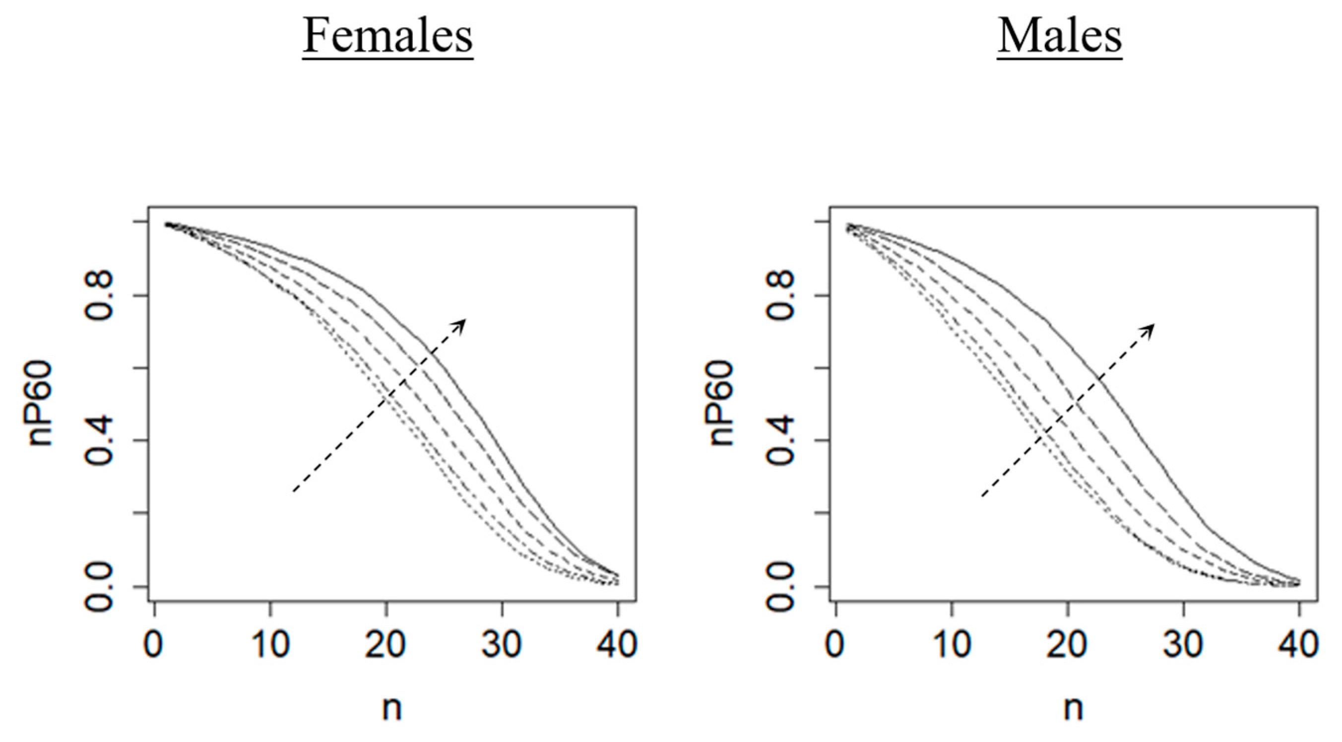
The continuous mortality decline, together with the lack of clear improvement in the maximum lifespan, has caused the common phenomenon of a “rectangularisation” of the survival curve. This kind of observations has been well documented in earlier studies (e.g., Fries 1980; Cheung et al. 2005). As shown in Figure 1, it can be characterised by an upward and rightward shift of the period survival curve across successive time periods. The increasing area under the survival curve over time refers to the extent of rectangularisation. This concept is one of the major analytical frameworks in demographic research and can actually be further adapted to describe past changes in survival levels and predict future survival rates. The recent developments in mortality projection methods can provide a useful reference for this direction of exploiting the trends in survival probabilities.
While there is a vast literature on modelling and projecting mortality rates (e.g., Lee and Carter 1992; Booth and Tickle 2008), relatively less attention has been paid on forecasting survival probabilities directly. Amongst the few previous works, De Jong and Marshall (2007) applied the probit link function to the survival probabilities of Australian females and assumed that it is driven by a single time trend. Hatzopoulos and Haberman (2015) used the complementary log-log link function and age-cohort effects within the GLM (generalised linear model) framework for the cohort survival probabilities of a few European countries. Wong and Tsui (2015) proposed a new survival function for US women and men and modelled the changes of its parameters over time by autoregressive processes. Tan et al. (2016) constructed a hybrid survival curve and applied the logit link function to the annualised survival probabilities with two or three sets of time-varying parameters using Swedish and Bulgarian data.
There are potential advantages of modelling and projecting the survival probabilities rather than the mortality rates. First, when producing life expectancy forecasts, it would be more convenient to work with the survival probabilities directly without having to compound the mortality rates to form the survival rates. In a similar vein, when pricing pensions or annuities, the future probabilities of survival are a major input for the calculation process, and so it would be more natural to build a projection model that focuses on the survival probabilities. Moreover, as shown in the following sections, the survival probability patterns and trends are generally quite stable, which make their forecasting more straightforward than otherwise. We will show in our empirical analysis that some of these survival rate projection models can actually outperform the more conventional approach of a mortality rate projection model.
As mentioned above, forecasting survival probabilities are much less explored in the literature when compared to forecasting mortality rates. In this paper, we attempt to reduce this knowledge gap by examining extensively a number of link functions on survival probabilities and modelling the evolution of the parameters and so the survival rates over time. The link functions considered include the probit, complementary log-log, logit, gevit functions, and a new link function based on the theory of minima, and both the age and period effects are incorporated. Furthermore, we illustrate how the survival rate projection models can be extended to include additional explanatory variables such as the GDP (gross domestic product) per capita. Some previous examples of incorporating macroeconomic factors into mortality rate projection models are Hanewald (2011); Niu and Melenberg (2014); French and O’Hare (2014); and Seklecka et al. (2019). To the best of our knowledge, our paper provides the first attempt to incorporate macroeconomic factors into the survival rate projection models.
The remainder of the papers is as follows. Section 2 gives an introduction of the various survival rate projection models being considered. Section 3 compares the fitting performances of the models for Australian and New Zealand data. Section 4 sets forth an out-of-sample analysis for measuring the forecasting performances of the models. Section 5 studies the potential link between the survival probabilities and the economic growth. Section 6 concludes.
2. Survival Rate Projection Models
Suppose is the mortality rate at age in year , and is the corresponding period survival probability in year for a surviving period of at least years. The first link function we consider is the probit function used by De Jong and Marshall (2007). We set the model structure as , in which is the inverse standard normal cdf (cumulative distribution function) and is a regression structure allowing for the age and period effects with . If one treats as the cdf of the future lifetime (within years) of a life aged in year , as the survival function of that future lifetime, and as a certain constant for , it can be deduced that and so . It then means that under this probit model structure, the future death rates can be seen as a Wang transform (Wang 2000) of the past death rates, with the parameter capturing the mortality decline. Note that the probit link function ensures that the survival rates are between 0 and 1, regardless of the values of , and that it is a symmetric link as approaches 0 and 1 at the same pace.
The next one is the complementary log-log link function used by Hatzopoulos and Haberman (2015). We follow their model structure as , that is, the link function is being applied on , but not . Unlike the probit function, the complementary log-log function is an asymmetric link, which would be useful for the rectangularisation patterns as in Figure 1. This asymmetry may suit survival modelling better when compared to a symmetric one. The survival rates under this link function are between 0 and 1.
We apply the logit link function from Tan et al. (2016) as . It is a symmetric link like the probit function, and it constrains the survival rates between 0 and 1. Its inverse function is actually the cdf of the logistic distribution with the location parameter equal to 0 and the scale parameter equal to 1. Both the probit and logit functions are used extensively in binary response models.
Recently, Medford and Vaupel (2019) proposed the so-called gevit link function for modelling mortality rates. We apply this link function differently here as ; that is, it is being applied on the survival probability but not on the death rate. This link is asymmetric and it constrains the survival rates like those above. Its inverse function is indeed the cdf of the GEV (generalised extreme value) distribution for maxima with the location parameter equal to 0 and the scale parameter equal to 1. The extra shape parameter provides more flexibility to manage the extent of asymmetry.
Inspired by the gevit link function, which is based on maxima, we exploit the GEV distribution for “minima” instead (e.g., Liu and Li 2019) as an alternative. The cdf of the minima GEV distribution is specified as . Accordingly, we consider a new model structure . It is straightforward to deduce that this new link is also asymmetric and the resulting survival rates are within the valid range. We refer to it as the “gevmin” model structure in the following analysis.
If this new link is applied on instead of , the model structure becomes . Then if , it reduces to , which means that the complementary log-log model structure above can effectively be seen as a specific example of this alternative model structure from minima.
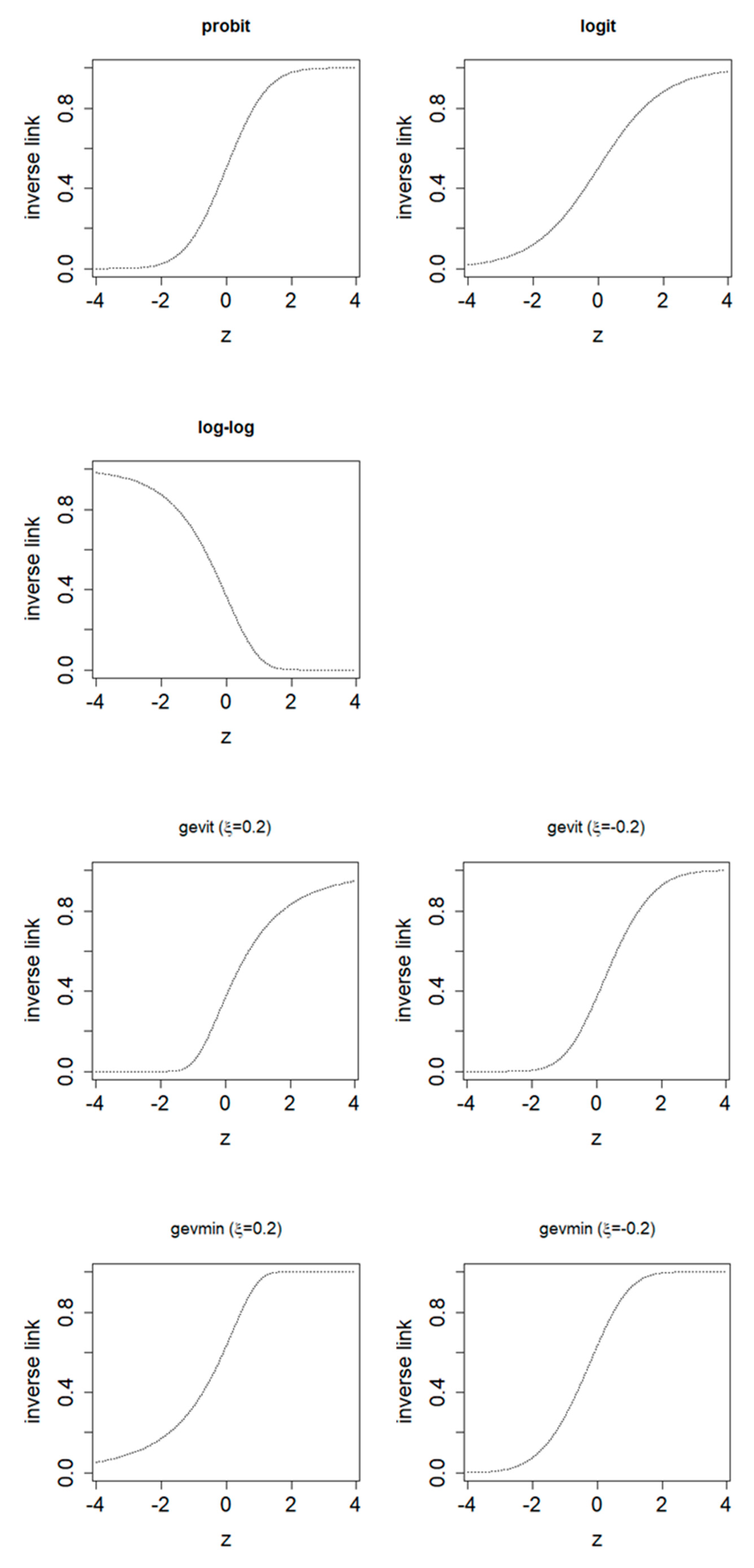
Figure 2 compares the symmetry of the probit and logit functions with the asymmetry of the complementary log-log, gevit, and gevmin functions as described above. For the symmetric ones, the response approaches 0 and 1 at the same pace. For the asymmetric complementary log-log and gevit functions, the response approaches 1 slower than reaching 0. By contrast, under the new gevmin model structure, the response of the (inverse) link approaches 1 faster than reaching 0, which is an opposite situation. As reflected in Figure 1, as the rectangularisation continues to occur, the survival rates of more and more ages rise above 0.5 and get closer to 1 over time , while the rates drop more and more sharply at the progressively narrowing highest end. This phenomenon may make one or more of the asymmetric candidates more suitable for modelling how the survival rates evolve over time. More details of the maxima and minima GEV distributions are given in the Appendix A.
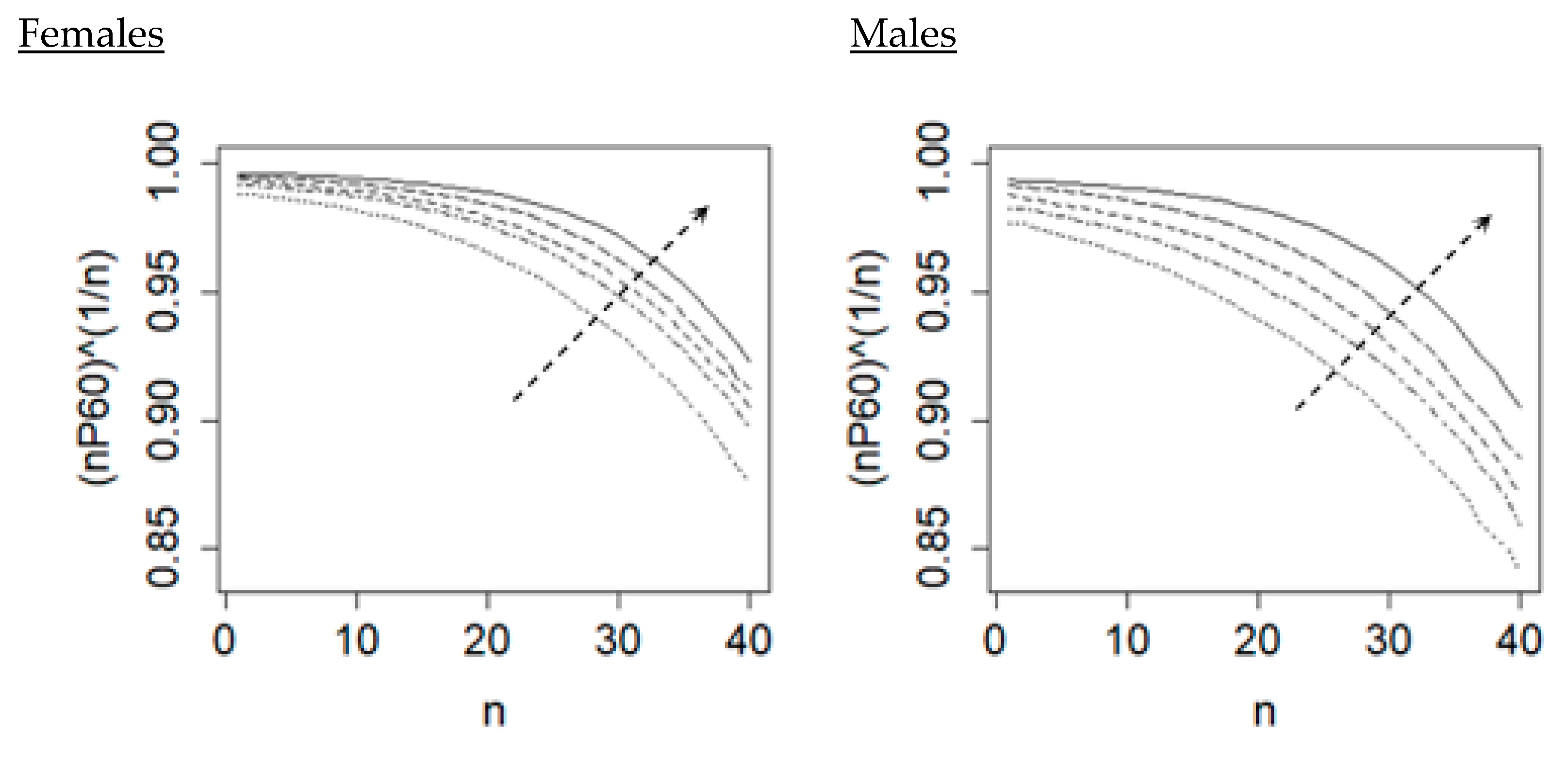
In addition to , we also follow Tan et al. (2016) and consider another response , that is, the “annualised” survival probability for comparison. Figure 3 shows that the resulting annualised survive curve also displays an upward and rightward shift over successive time periods. Regarding the regression structure , we employ both the Lee and Carter (1992) structure and the Cairns et al. (2009) structure to allow for the age and period effects. The first one is taken as , and the second one as , where is the age effect, is the “survival index” with age-specific sensitivity , to are three time-varying parameters, is the average of the age range, and is the average of over the age range considered. Altogether, there are 5 (links) × 2 (responses) × 2 (structures) = 20 combinations under our consideration. This coverage is much more comprehensive than those of the few earlier papers on projecting the survival rates directly. Subsequently, we will also explore adding macroeconomic factors into the regression structure to see whether it can improve the performances. The Appendix A provides the parameter estimation methods for the models tested.
Note that some of these stochastic projection models can be seen as modifications of those standard static mortality or survival functions. Suppose and represent the force of mortality and the t-year survival rate of a life aged x for a static one-year life table. For instance, the Gompertz law states that , which can be transformed into the survival function and a regression structure . The old-age component of the Heligman–Pollard curve can be taken as , which can be expressed as the survival function and a regression structure . The famous Lee–Carter model (Lee and Carter 1992) and the CBD model (Cairns et al. 2006) can be seen in some way as adding time-varying components into the two regression structures above (log and logit) in order to turn them from being static to stochastic. While the stochastic Lee–Carter and CBD models deal with mortality rates, as compared to our approach of modelling survival probabilities, we will include them in the following analysis for comparison.
3. Fitting Performances
In this section, we apply the 20 models (combinations) to female and male populations in Australia and New Zealand. The mortality data of ages 60 to 99 and years 1970 to 2017 of Australia (1970 to 2013 for New Zealand) are extracted from the Human Mortality Database (HMD 2020). For demonstration purposes, we consider the survival probabilities for a life aged 60 and set (for surviving periods = 1, 2, 3, …, 40), as the mortality rates below age 60 have already reached very low levels and have relatively little impact on the overall survival rates. In fact, the survival rate of a newborn for a surviving period up to 60 years is now very close to one, and the corresponding movements over time look too insignificant for a meaningful projection. By contrast, there is still much room for the survival rates at ages 60 and above to improve, and as shown below, the resulting patterns and trends are rather stable and can readily be projected into the future. Moreover, longevity of retirees is a serious concern for governments, insurers selling annuities, and pension funds because of the increasing financial burden. It would be of high practical interest to focus on the mortality of retirement ages.
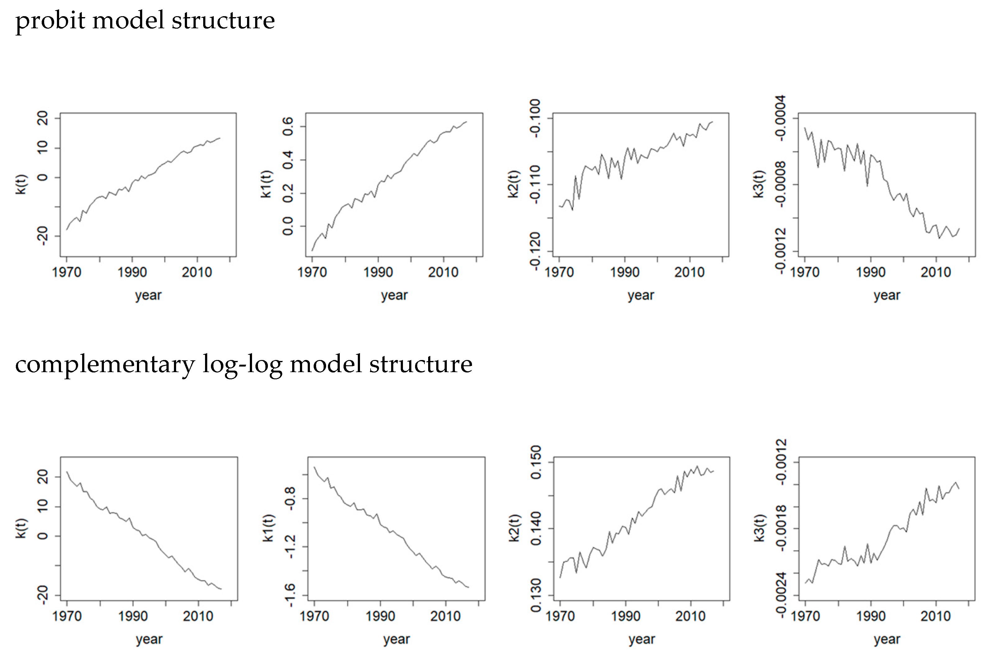
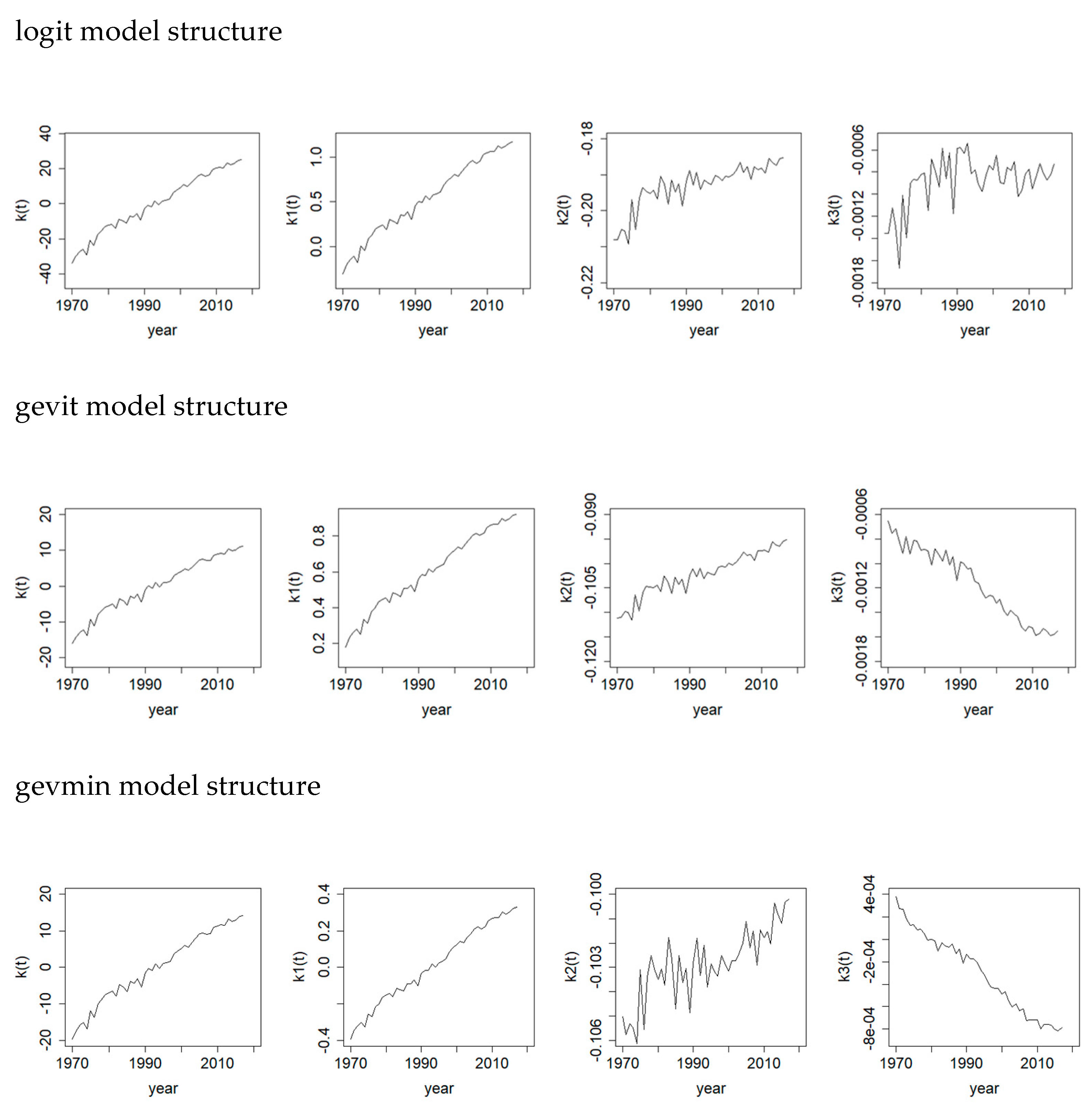
Figure 4 plots the survival index of the first regression structure and also the time-varying parameters to of the second regression structure based on the five different link functions for the survival probabilities of Australian females. It is interesting to see that all the temporal parameters of and demonstrate a strong linearly increasing trend. It reflects clearly the continually improving survival rates at old ages as a whole. (For the complementary log-log model structure, Figure 2 displays a negative relationship between the response and the argument in contrast to the others. The resulting major trends of and in Figure 4 are then inverted, but the implication on mortality decline is the same.) The time-varying parameters and of the second regression structure refer to the slope and curvature in year . While the directions of their trends are different because of the differences in how the link functions operate on the survival rates, a high level of linearity can largely be observed. We can then use the (univariate or multivariate) random walk with drift to project all these linear trends. Compared to the time-varying trends usually seen when modelling the mortality rates (e.g., Cairns et al. 2009), modelling the survival rates here generates more linear trends, which make the use of the random walk with drift more justifiable than otherwise. The observations for Australian male and New Zealand populations (not shown here) exhibit similar patterns.
Table 1 reports the MAPE (mean absolute percentage error) values on of fitting the 20 models, with the original Lee–Carter model (Lee and Carter 1992) and the CBD model with curvature (Cairns et al. 2009) for the death rates also included for comparison. The major observations are stated below:
- (1)
- For the first regression structure, the MAPE values are often smaller when the response is . By contrast, for the second regression structure, the MAPEs are much smaller when the response is .
- (2)
- When the response is , the MAPE values from the first regression structure are clearly smaller. However, when the response is , the situation is mostly reversed.
- (3)
- For the complementary log-log model structure with the first regression form, the MAPE remains the same regardless of the response (i.e., or ). The underlying reason is that is indeed equivalent to , where . Hence, they produce the same fitted values of and so the same MAPEs.
- (4)
- Overall, the combination of the response and the second regression structure (i.e., ) gives the better MAPEs. In particular, the gevmin model structure, based on the newly proposed gevmin link, leads to the smallest MAPEs consistently for all the populations (0.73, 0.93, 1.20, 1.68) considered.
- (5)
- The best gevmin model structures noted above outperform the more traditional approaches of the Lee–Carter and CBD models in modelling the mortality rates (with MAPEs of 1.39 to 3.02).
Compared with the traditional link functions, the additional shape parameter in the gevmin and gevit link functions makes them a lot more flexible in capturing different degrees of asymmetry. For each population in Table 1, the two smallest MAPEs are all generated from either the gevmin or gevit model structure. The empirical advantage of using these two newer links is apparent here. Note also that the response (see Figure 3 again) has a simpler shape over than the response (see Figure 1). Hence, a simple regression structure in terms of merely (i.e., ) would suffice for the former, while a more dedicated allowance for the age effect (i.e., ) would be needed for the latter.
As noted earlier, if the new gevmin link is applied on rather than , the model structure turns into . It can further be rearranged as , which then becomes the gevit model structure effectively. Consequently, they generate the same fitted values of and the same MAPEs, though the resulting signs and trends of their parameters are opposite to each other. However, the increasing survival index based on the gevmin link on has a more natural interpretation in terms of improving survival over time.
4. Forecasting Performances
In this section, we perform an out-of-sample analysis to assess the forecast accuracy of the survival rate projection models. We apply the models to four fitting periods of 1970 to 1989 (20 years), 1970 to 1994 (25 years), 1970 to 1999 (30 years), and 1970 to 2004 (35 years) and then forecast the survival rates for the remaining periods until the very last year of available data. Here we focus on the annualised response and the second regression structure since they give the better fitting performances in Table 1. In addition to continuing to use the Lee–Carter and CBD models for comparison, we also apply the multivariate random walk with drift to the survival probabilities as a benchmark, naive model. The MAPEs of not only the projected but also the projected life expectancies at age 60 are examined to compare the performances. They are calculated as and respectively, where and ( and ) are the projected and observed survival probabilities (life expectancies) in year , is the number of data points, and is the number of years in the testing period. For each case (column) in Table 2, the three lowest MAPE values are highlighted (in grey). We notice the following patterns within the results in Table 2:
- (1)
- Out of the 16 cases (4 fitting periods × 2 countries × 2 sexes), the gevit and gevmin model structures produce the three lowest MAPEs in 12 cases. Their performances are the most consistent ones amongst all the candidates.
- (2)
- For the gevit and gevmin model structures, the average MAPE is 6.10. For the probit, complementary log-log, and logit model structures, the average MAPE is 6.29. For the LC and CBD models, the average MAPE is 6.53. For the naive random walk model, the average MAPE is 7.95.
- (3)
- The MAPE values tend to be lower for females (4.04 on average) than for males (8.98 on average).
- (4)
- The MAPE values tend to be lower for Australia (5.65 on average) than for New Zealand (7.36 on average).
- (5)
- The naive random walk model leads to the highest MAPE values in 10 cases.
Overall, the gevit and gevmin model structures deliver the best and the most consistent forecasting performances among the eight alternatives. Moreover, the survival rate projection models as a whole also tend to outperform the usual Lee–Carter and CBD models in this out-of-sample analysis of the survival rates. These results highlight the potential usefulness of projecting the survival rates directly when the focus is on the survival probabilities. The generally poor performances by the naive random walk model also emphasise the importance of having a proper model structure for modelling the survival rates.
Regarding the MAPEs of the projected life expectancies in Table 3, the gevit and gevmin model structures continue to perform well relative to the others. Their average MAPE is 2.31, compared to 2.56 for the probit, complementary log-log, and logit model structures and 2.81 for the LC and CBD models. It highlights again the flexibility offered by the extra shape parameter and the potential benefits. Moreover, the survival rate projection models still perform better than the Lee–Carter and CBD models in general. Projecting the survival rates directly would be a useful strategy or alternative if the main task is to forecast future life expectancies. It is also interesting to note that the average MAPE for the naive random walk model is only 2.44. We conjecture that their larger errors as shown in Table 2 may have coincidently offset one another to some extent across different ages as life expectancy is effectively an aggregate measure of survival probabilities. Anyway, the advantages of imposing an appropriate model structure are obvious in modelling the survival rates.
In addition to the MAPE values, the sMAPE (symmetric mean absolute percentage error) values are also calculated and given in the Appendix A. The major implications are largely the same as those discussed above.
5. The Effect of Economic Growth
There have been previous studies in the area of demography and macroeconomics showing the impact of economic fluctuations on mortality levels (e.g., Ruhm 2000; Brenner 2005). A few earlier papers in mortality projection that incorporated exogenous economic factors include Hanewald (2011), Niu and Melenberg (2014), and Boonen and Li (2017). They showed that the Gross Domestic Product (GDP) of a nation may serve as an explanatory factor of a country’s mortality rates. Furthermore, they demonstrated that it may be integrated into extrapolative mortality models such as the Lee–Carter model or its extensions to improve the fitting quality. In this section, we experiment with embedding such macroeconomic factor into the survival rate projection models. As a preliminary analysis, we find some positive correlation ( = 0.17 for Australian females, 0.10 for Australian males, 0.08 for New Zealand females, 0.15 for New Zealand males) between the annual change in survival index and the annual growth in real GDP per capita for the period from 1970 onwards (for Australia and New Zealand respectively). The survival index can be seen as an underlying driver of the survival probabilities and so an indicator of how life expectancy changes, and the GDP trend is a very important indicator of economic growth. This observation provides some incentive for putting the survival trend and the economic trend together into the modelling framework. By doing so, the extended model may produce more interpretable implications on the projected survival rates based on the projected economic growth. In effect, such a model can be regarded as partly extrapolative (using past survival trends) and partly explanatory (using exogenous GDP figures). Note that the GDP can be regarded as an overall indicator of the quality of life. As the focus of our study is the use of new link functions in modelling survival probabilities and the aggregate data used are of country level, we deem that the GPD itself would be sufficient for our analysis1.
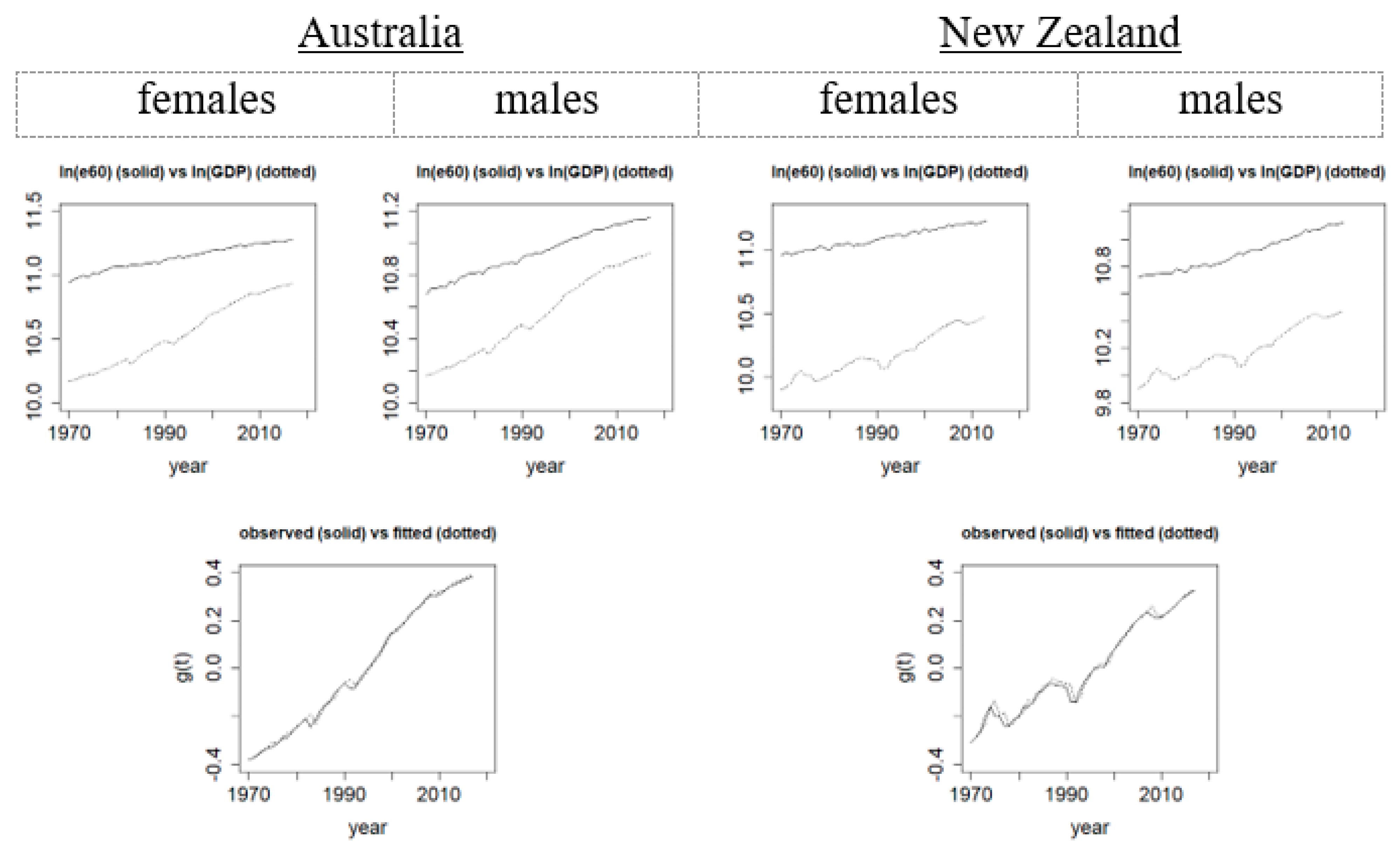
Accordingly, we modify the first regression structure as , in which is the (log) real GDP per capita in year and is the (age-specific) associated coefficient. The values of are adjusted such that , and so still refers to the overall (average over time) age effect. The real GDP per capita data are obtained from World Development Indicators (WDI 2020), the primary database maintained by World Bank on comparative development indicators across countries worldwide. Figure 5 (upper panel) illustrates the increasing trend of the GDP in recent decades, as well as some potential co-movements with the life expectancy trend. Following the Box and Jenkins (1976) approach, we find that the ARIMA(1,1,0) process (autoregressive integrated moving-average) provides an adequate description of the dynamics of the GDP process. Figure 5 (lower panel) also shows that the fitted GDP values from ARIMA(1,1,0) are very close to the observed values.
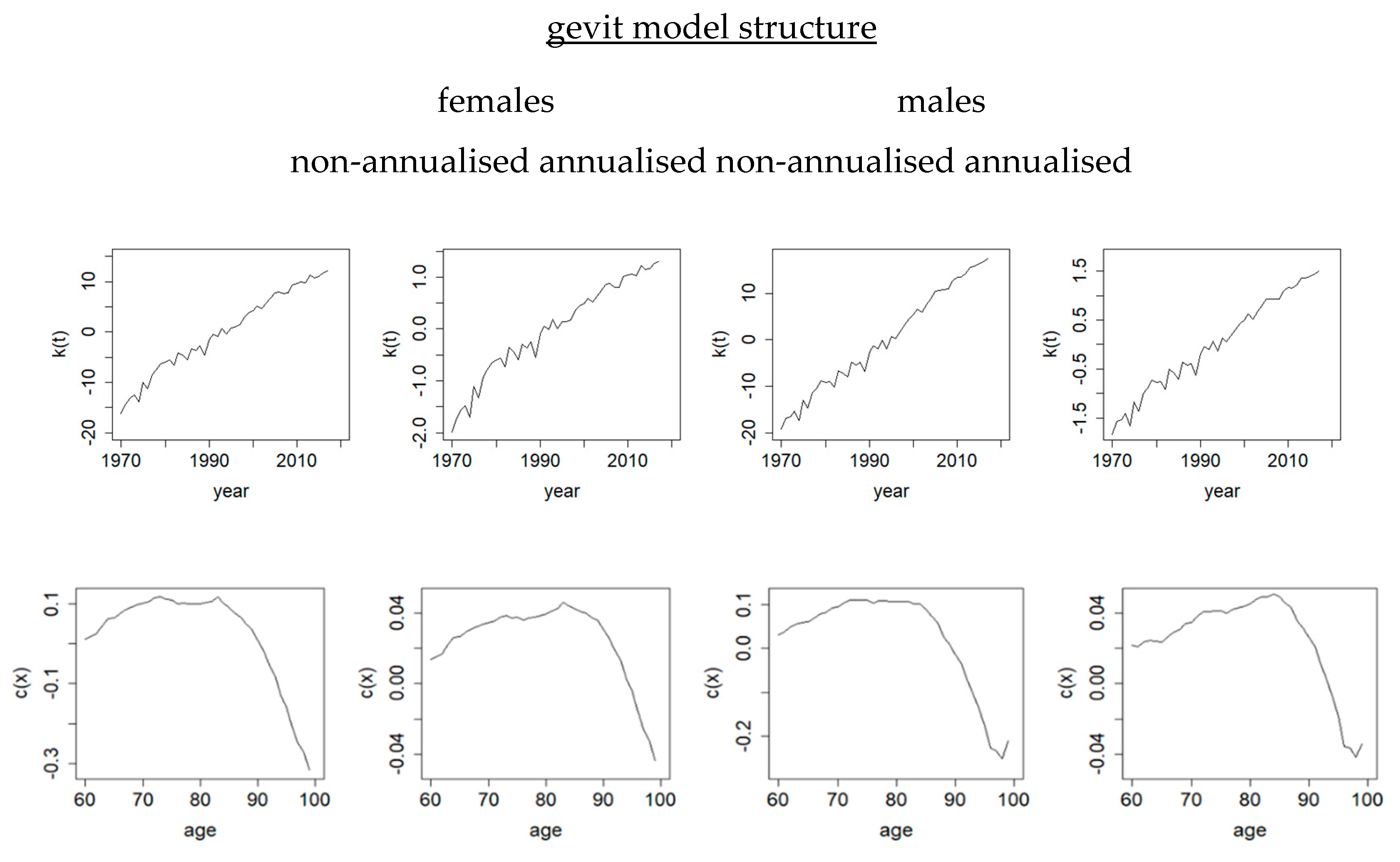
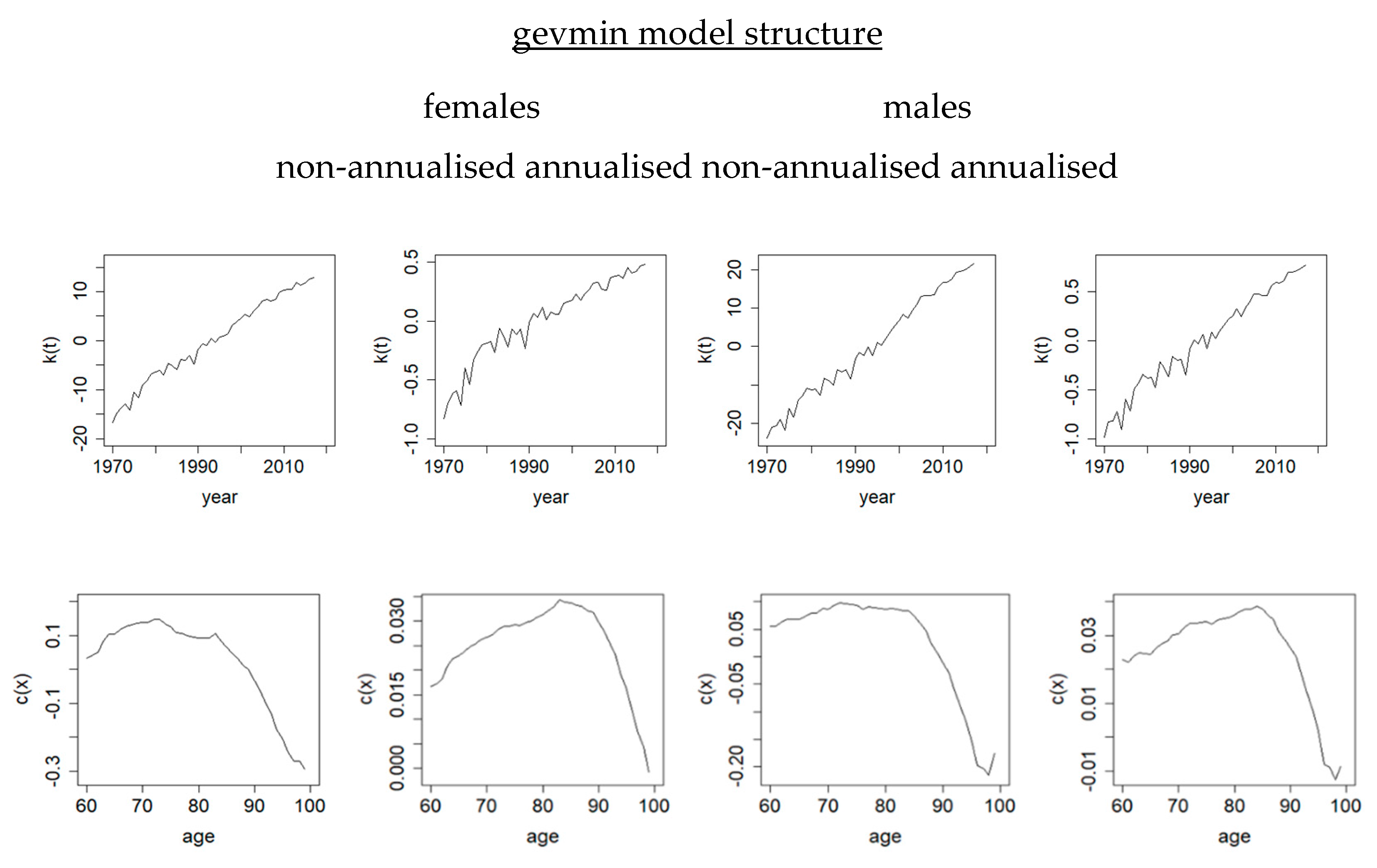
Figure 6 plots the survival indices under the modified (with GDP) first regression structure with the gevit and gevmin links. While the new factor is supposed to explain part of the rising survival trend, the computed survival indices still exhibit a clear linearly increasing trend, though their drifts (around 0.37) are smaller than previously (about 0.43 without the GDP factor). It is also interesting to see in Figure 6 that the age-sensitivity is high at ages 60 to 80 but it drops drastically after around age 80, reflecting that the very-old-age mortality is still much less responsive to economic growth (likely due to current technological and medical limitations).
Table 4 compares the fitting performances with and without the GDP factor. Interestingly, all the MAPE values become smaller after incorporating the GDP covariate. Furthermore, Table 5 and Table 6 present the forecasting performances before and after embedding the GDP covariate under the same out-of-sample test setting as in Section 4. For both the projected survival probabilities and the projected life expectancies at age 60, adding the GDP factor leads to a clear improvement in forecast accuracy in most of the cases. It is obvious that besides the selection of appropriate link function, age and period effects, and annualisation of the survival rates, integrating a GDP explanatory factor within the model has much potential in further enhancing the performance of a survival rate projection model.
A final note is that while our regression structure here is designed to examine how the economic trend would affect and/or move synchronously along with the survival trend over the long term, we acknowledge that the underlying process can be more complicated in terms of the direction of causation and the lagging effect. These matters are beyond the scope of this paper and we leave them for future research.
6. Concluding Remarks
In this paper, we have conducted a thorough examination on several old and new link functions for their applications in modelling how old-age survival probabilities evolve across time in Australasia. The link functions under investigation include the newly proposed gevit and gevmin links, which are compared against the traditional ones like probit, complementary log-log, and logit links. We use the random walk with drift to project the temporal parameters due to their highly linear trends in the past decades. Future survival probabilities and life expectancies are then projected using the estimated parameters. We notice that many of these survival rate projection models can produce better fitting and forecasting performances than the more conventional approach of modelling mortality rates, in terms of achieving lower MAPE and sMAPE values. Hence, projecting the survival rates directly would serve as a useful strategy or alternative if the objective is to forecast future life expectancies. In particular, the gevmin and gevit links are found to be able to offer extra flexibility in depicting the (annualised or non-annualised) survival curve patterns and improve the model performance. This extra flexibility comes from the additional shape parameter that copes with any extent of asymmetry. Lastly, we illustrate how these survival rate projection models can be modified to incorporate additional explanatory variables, in an attempt to further enhance the model results. We notice that adding a covariate on the real GDP per capita can improve the general fitting performances as well as many of the forecasting performances. Note that our approach can be applied similarly to other ages above 60 for . The focus of this work is on forecasting survival probabilities at ages 60 and above, as the current death rates below age 60 are very low and their impact on the overall survival rates has become much less important. If one is interested in modelling the entire age range, the Lee–Carter model and its various extensions in modelling mortality rates can be used instead.
There are two potential areas for future research. First, since a link function is often constructed from the inverse of a cdf, the use of other cdfs can be explored. There are a range of skewed distributions which may be useful for tackling different levels of asymmetry. Second, while we have used two particular regression forms in our analysis, there are other possible structures that also allow for the age and period effects. Some examples include adding extra time-varying parameters and co-modelling the survival rates of related subpopulations.
Funding
This research received no external funding.
Institutional Review Board Statement
Not applicable.
Informed Consent Statement
Not applicable.
Data Availability Statement
Not applicable.
Conflicts of Interest
The author declares no conflict of interest.
Appendix A
Suppose , , …, are independent and identically distributed (i.i.d.) random variables having cdf . Let be the maximum value amongst them. Under the Fisher–Tippett–Gnedenko Theorem and certain technical conditions, when goes to infinity, (for some and real ) follows the so-called distribution (for and ). There are three specific cases: Gumbel (), Fréchet (), and reversed Weibull (). Their cdfs are, respectively,
Let be the corresponding minimum value. Under some technical conditions, with approaching infinity, follows the distribution (for and ). There are also three specific cases: reversed Gumbel (), reversed Fréchet (), and Weibull (). Their cdfs are, respectively,
The SVD (singular value decomposition) method is employed to estimate the parameters in . Regarding , the least squares method is used to estimate the parameters for each year . When there exists a shape parameter , an extensive range of different trial values are taken for it in turn and then different sets of parameter values are estimated accordingly. The final value of the shape parameter is determined by the one giving the smallest overall fitting error. Table A1 below provides the final values of the shape parameter for different populations and fitting periods. All the estimated values are negative, implying that the GEV distribution involved belongs to the reversed Weibull. For the second regression structure (right value), all the estimated values are quite consistent with one another, ranging from about −0.4 to −0.3. For the first regression structure (left value), the estimated values range from −0.6 to −0.5 when the response is and are −1.1 to −0.8 when the response is . Note that these estimation approaches are adopted in this paper because each response depends on the mortality rates of ages, so it is impossible to apply the Poisson assumption via maximum likelihood that is commonly used with mortality rate projection models.

Table A1.
Estimated shape parameter values of gevit model structure fitted to Australian and New Zealand data (left value—first regression structure; right value—second regression structure).
Table A1.
Estimated shape parameter values of gevit model structure fitted to Australian and New Zealand data (left value—first regression structure; right value—second regression structure).
| Fitting Period | Australian Females | Australian Males | ||
| Non-Annualised | Annualised | Non-Annualised | Annualised | |
| 1970–2017 | −0.59/−0.32 | −0.85/−0.31 | −0.60/−0.39 | −0.93/−0.30 |
| 1970–1999 | −0.66/−0.35 | −0.99/−0.42 | −0.62/−0.45 | −1.08/−0.40 |
| 1970–1989 | −0.57/−0.34 | −0.89/−0.37 | −0.62/−0.43 | −1.06/−0.37 |
| Fitting Period | New Zealand Females | New Zealand Males | ||
| Non-Annualised | Annualised | Non-Annualised | Annualised | |
| 1970–2013 | −0.58/−0.34 | −0.90/−0.31 | −0.53/−0.41 | −0.86/−0.35 |
| 1970–1999 | −0.54/−0.37 | −0.83/−0.37 | −0.48/−0.45 | −0.86/−0.45 |
| 1970–1989 | −0.55/−0.36 | −0.86/−0.36 | −0.53/−0.43 | −0.91/−0.38 |
As noted in Hyndman and Koehler (2006), the MAPE would have the disadvantage of putting a heavier penalty on positive errors than on negative errors. Accordingly, the sMAPE values are also calculated and reported in Table A2 and Table A3 below. Regarding the sMAPEs of the projected survival probabilities in Table A2, the average sMAPE is 6.57 for the gevit and gevmin model structures, compared to 7.01 for the probit, complementary log-log, and logit model structures, 6.93 for the LC and CBD models, and 9.23 for the naive random walk model. Regarding the sMAPEs of the projected life expectancies in Table A3, the average sMAPE is 2.35 for the gevit and gevmin model structures, compared to 2.62 for the probit, complementary log-log, and logit model structures, 2.89 for the LC and CBD models, and 2.50 for the naive random walk model. The gevit and gevmin model structures contribute to the three lowest sMAPEs in 11 or 12 of the 16 cases, and overall, they show the best forecasting performances in our out-of-sample analysis on the survival rates.
Table A2.
sMAPE values (%) on projected survival probabilities at age 60 using Australian and New Zealand data for different fitting periods.
Table A2.
sMAPE values (%) on projected survival probabilities at age 60 using Australian and New Zealand data for different fitting periods.
| Australian Females | Australian Males | |||||||
| Model | 1970–1989 | 1970–1994 | 1970–1999 | 1970–2004 | 1970–1989 | 1970–1994 | 1970–1999 | 1970–2004 |
| probit | 5.79 | 1.87 | 2.89 | 2.90 | 17.67 | 11.25 | 2.76 | 1.67 |
| log-log | 6.91 | 2.13 | 2.60 | 1.98 | 18.82 | 12.39 | 3.64 | 1.63 |
| logit | 6.71 | 2.03 | 2.58 | 2.70 | 18.59 | 12.16 | 3.42 | 2.06 |
| gevit | 4.75 | 2.52 | 3.91 | 3.68 | 16.27 | 10.01 | 2.41 | 2.04 |
| gevmin | 4.75 | 2.35 | 3.67 | 3.49 | 16.73 | 10.40 | 2.41 | 1.74 |
| LC | 3.92 | 3.08 | 3.00 | 2.29 | 11.72 | 8.07 | 4.13 | 3.33 |
| CBD | 4.90 | 1.89 | 3.10 | 3.32 | 18.49 | 12.58 | 3.82 | 2.34 |
| MRW | 9.88 | 4.72 | 2.52 | 2.03 | 23.17 | 17.20 | 8.55 | 5.87 |
| New Zealand Females | New Zealand Males | |||||||
| Model | 1970–1989 | 1970–1994 | 1970–1999 | 1970–2004 | 1970–1989 | 1970–1994 | 1970–1999 | 1970–2004 |
| probit | 5.06 | 5.21 | 3.41 | 2.90 | 15.20 | 9.25 | 10.79 | 9.36 |
| log-log | 5.56 | 4.76 | 3.68 | 3.49 | 15.75 | 9.79 | 11.41 | 9.90 |
| logit | 5.44 | 4.84 | 3.60 | 3.35 | 15.63 | 9.68 | 11.27 | 9.78 |
| gevit | 4.97 | 5.65 | 3.55 | 2.95 | 14.36 | 8.57 | 10.16 | 8.97 |
| gevmin | 4.98 | 5.67 | 3.55 | 2.93 | 14.64 | 8.83 | 10.35 | 9.04 |
| LC | 6.37 | 6.21 | 4.92 | 3.35 | 18.57 | 10.26 | 9.43 | 6.82 |
| CBD | 5.64 | 7.00 | 3.78 | 2.91 | 16.41 | 9.92 | 11.40 | 8.73 |
| MRW | 7.19 | 3.15 | 3.80 | 3.57 | 18.79 | 12.51 | 13.26 | 11.39 |
Table A3.
sMAPE values (%) on projected life expectancies at age 60 using Australian and New Zealand data for different fitting periods.
Table A3.
sMAPE values (%) on projected life expectancies at age 60 using Australian and New Zealand data for different fitting periods.
| Australian Females | Australian Males | |||||||
| Model | 1970–1989 | 1970–1994 | 1970–1999 | 1970–2004 | 1970–1989 | 1970–1994 | 1970–1999 | 1970–2004 |
| probit | 1.69 | 0.69 | 1.11 | 1.19 | 5.51 | 3.75 | 0.84 | 0.55 |
| log-log | 2.02 | 0.71 | 0.87 | 1.02 | 6.10 | 4.33 | 1.35 | 0.39 |
| logit | 1.99 | 0.71 | 0.89 | 1.04 | 6.03 | 4.27 | 1.29 | 0.40 |
| gevit | 1.25 | 0.95 | 1.59 | 1.50 | 4.44 | 2.74 | 0.66 | 1.02 |
| gevmin | 1.35 | 0.81 | 1.41 | 1.37 | 4.98 | 3.28 | 0.66 | 0.77 |
| LC | 2.07 | 0.74 | 0.79 | 0.81 | 6.33 | 4.22 | 1.56 | 0.70 |
| CBD | 2.25 | 0.79 | 0.78 | 0.99 | 6.63 | 4.63 | 1.70 | 0.52 |
| MRW | 1.34 | 0.79 | 1.41 | 1.47 | 5.20 | 3.47 | 0.74 | 0.68 |
| New Zealand Females | New Zealand Males | |||||||
| Model | 1970–1989 | 1970–1994 | 1970–1999 | 1970–2004 | 1970–1989 | 1970–1994 | 1970–1999 | 1970–2004 |
| probit | 2.88 | 0.75 | 1.80 | 1.18 | 7.49 | 4.41 | 4.19 | 2.22 |
| log-log | 2.98 | 0.81 | 1.85 | 1.15 | 7.79 | 4.71 | 4.42 | 2.36 |
| logit | 2.97 | 0.80 | 1.85 | 1.15 | 7.75 | 4.67 | 4.40 | 2.35 |
| gevit | 2.67 | 0.78 | 1.65 | 1.16 | 6.89 | 3.88 | 3.78 | 1.93 |
| gevmin | 2.74 | 0.75 | 1.72 | 1.19 | 7.16 | 4.14 | 3.98 | 2.10 |
| LC | 3.57 | 0.92 | 2.41 | 1.13 | 9.87 | 5.46 | 4.64 | 2.27 |
| CBD | 3.18 | 0.80 | 1.80 | 1.17 | 7.70 | 4.93 | 4.47 | 2.57 |
| MRW | 3.19 | 0.80 | 1.76 | 1.15 | 7.51 | 4.37 | 4.06 | 2.03 |
References
- Boonen, Tim J., and Hong Li. 2017. Modeling and forecasting mortality with economic growth: A multipopulation approach. Demography 54: 1921–46. [Google Scholar] [CrossRef] [PubMed]
- Booth, Heather, and Leonie Tickle. 2008. Mortality modelling and forecasting: A review of methods. Annals of Actuarial Science 3: 3–43. [Google Scholar] [CrossRef]
- Box, George E. P., and Gwilym M. Jenkins. 1976. Time Series Analysis: Forecasting and Control, 2nd ed. San Francisco: Holden-Day. [Google Scholar]
- Brenner, Harvey M. 2005. Commentary: Economic growth is the basis of mortality rate decline in the 20th century: Experience of the United States 1901–2000. International Journal of Epidemiology 34: 1214–21. [Google Scholar] [CrossRef] [PubMed]
- Cairns, Andrew J. G., David Blake, and Kevin Dowd. 2006. A two-factor model for stochastic mortality with parameter uncertainty: Theory and calibration. Journal of Risk and Insurance 73: 687–718. [Google Scholar] [CrossRef]
- Cairns, Andrew J. G., David Blake, Kevin Dowd, Guy D. Coughlan, David Epstein, Alen Ong, and Igor Balevich. 2009. A quantitative comparison of stochastic mortality models using data from England and Wales and the United States. North American Actuarial Journal 13: 1–35. [Google Scholar] [CrossRef]
- Cheung, Siu Lan Karen, Jean-Marie Robine, Edward Jow-Ching Tu, and Graziella Caselli. 2005. Three dimensions of the survival curve: Horizontalization, verticalization, and longevity extension. Demography 42: 243–58. [Google Scholar] [CrossRef]
- De Jong, Piet, and Claymore Marshall. 2007. Mortality projection based on the Wang transform. ASTIN Bulletin 37: 149–61. [Google Scholar] [CrossRef] [Green Version]
- French, Declan, and Colin O’Hare. 2014. Forecasting death rates using exogenous determinants. Journal of Forecasting 33: 640–50. [Google Scholar] [CrossRef]
- Fries, James F. 1980. Aging, natural death, and the compression of morbidity. New England Journal of Medicine 303: 130–35. [Google Scholar] [CrossRef] [Green Version]
- Hanewald, Katja. 2011. Explaining mortality dynamics. North American Actuarial Journal 15: 290–314. [Google Scholar] [CrossRef]
- Hatzopoulos, Petros, and Steven Haberman. 2015. Modeling trends in cohort survival probabilities. Insurance: Mathematics and Economics 64: 162–79. [Google Scholar] [CrossRef]
- HMD (Human Mortality Database). 2020. Berkeley and Rostock: University of California, Berkeley, and Max Planck Institute for Demographic Research. Available online: http://www.mortality.org/ (accessed on 28 December 2020).
- Hyndman, Rob J., and Anne B. Koehler. 2006. Another look at measures of forecast accuracy. International Journal of Forecasting 22: 679–88. [Google Scholar] [CrossRef] [Green Version]
- Lee, Ronald D., and Lawrence R. Carter. 1992. Modeling and forecasting U.S. mortality. Journal of the American Statistical Association 87: 659–71. [Google Scholar] [CrossRef]
- Lee, Ronald D., Lawrence Carter, and Shripad Tuljapurkar. 1995. Disaggregation in population forecasting: Do we need it? And how to do it simply. Mathematical Population Studies 5: 217–34. [Google Scholar] [CrossRef] [PubMed]
- Liu, Jia, and Jackie Li. 2019. Beyond the highest life expectancy—Construction of proxy upper and lower life expectancy bounds. Journal of Population Research 36: 159–81. [Google Scholar] [CrossRef]
- Medford, Anthony, and James W. Vaupel. 2019. An introduction to gevistic regression mortality models. Scandinavian Actuarial Journal 2019: 604–20. [Google Scholar] [CrossRef]
- Nikolaevich, Khubaev Georgy. 2019. How to Increase Duration of the Population of the Country. Beijing: Scientific Research of the SCO Countries: Synergy and Integration. [Google Scholar]
- Niu, Geng, and Bertrand Melenberg. 2014. Trends in mortality decrease and economic growth. Demography 51: 1755–73. [Google Scholar] [CrossRef]
- Oeppen, Jim, and James W. Vaupel. 2002. Broken limits to life expectancy. Science 296: 1029–31. [Google Scholar] [CrossRef] [Green Version]
- Ruhm, Christopher J. 2000. Are recessions good for your Health? Quarterly Journal of Economics 115: 617–50. [Google Scholar] [CrossRef]
- Seklecka, Malgorzata, Norazliani Md. Lazam, Athanasios A. Pantelous, and Colin O’Hare. 2019. Mortality effects of economic fluctuations in selected eurozone countries. Journal of Forecasting 38: 39–62. [Google Scholar] [CrossRef] [Green Version]
- Tan, Chong It, Jackie Li, Johnny Siu-Hang Li, and Uditha Balasooriya. 2016. Stochastic modelling of the hybrid survival curve. Journal of Population Research 33: 307–31. [Google Scholar] [CrossRef] [Green Version]
- Wang, Shaun S. 2000. A class of distortion operations for pricing financial and insurance risks. Journal of Risk and Insurance 67: 15–36. [Google Scholar] [CrossRef] [Green Version]
- WDI (World Development Indicators). 2020. World Bank Open Data- World Development Indicators Database. Washington, DC: The World Bank, Available online: https://data.worldbank.org/ (accessed on 28 December 2020).
- Wong, Chi Heem, and Albert K. Tsui. 2015. Forecasting life expectancy: Evidence from a new survival function. Insurance: Mathematics and Economics 65: 208–26. [Google Scholar] [CrossRef] [Green Version]
| 1 | In future research, if mortality and social data are available at finer levels such as social deprivation groups and subpopulations, other indicators like income, education, and smoking status can be added to the analysis. |
Figure 1.
Survival curves of New Zealanders aged 60 in 1970, 1980, 1990, 2000, and 2013.

Figure 2.
Five different (inverse) link functions.

Figure 3.
Annualised survival curves of Australians aged 60 in 1970, 1980, 1990, 2000, and 2017.

Figure 4.
Trends of and to based on five link functions for non-annualised survival probabilities of Australian females.
Figure 4.
Trends of and to based on five link functions for non-annualised survival probabilities of Australian females.


Figure 5.
Trends of life expectancy at age 60, national GDP, and gt of Australia and New Zealand.

Figure 6.
Trends of and age-sensitivity to GDP based on gevit and gevmin link functions for annualised and non-annualised survival probabilities of Australian females and males.
Figure 6.
Trends of and age-sensitivity to GDP based on gevit and gevmin link functions for annualised and non-annualised survival probabilities of Australian females and males.


Table 1.
MAPE values (%) on fitted survival probabilities at age 60 from fitting 22 models to Australian and New Zealand data (1970–2017 and 1970–2013 respectively).
Table 1.
MAPE values (%) on fitted survival probabilities at age 60 from fitting 22 models to Australian and New Zealand data (1970–2017 and 1970–2013 respectively).
| Model | Australian Females | Australian Males | ||
| Non-Annualised | Annualised | Non-Annualised | Annualised | |
| 1.24 | 1.47 | 2.03 | 2.53 | |
| 1.59 | 1.59 | 2.75 | 2.75 | |
| 1.39 | 1.59 | 1.94 | 2.72 | |
| 1.11 | 1.09 | 1.91 | 2.00 | |
| 1.12 | 1.14 | 1.82 | 1.87 | |
| 4.38 | 1.14 | 5.76 | 1.12 | |
| 7.20 | 2.17 | 11.74 | 1.80 | |
| 8.49 | 1.96 | 11.76 | 1.60 | |
| 2.71 | 0.85 | 3.48 | 1.01 | |
| 2.95 | 0.73 | 3.71 | 0.93 | |
| Lee-Carter | 1.39 | 2.42 | ||
| CBD | 1.62 | 1.57 | ||
| Model | New Zealand Females | New Zealand Males | ||
| Non-Annualised | Annualised | Non-Annualised | Annualised | |
| 2.23 | 2.61 | 2.76 | 3.11 | |
| 2.82 | 2.82 | 3.27 | 3.27 | |
| 2.36 | 2.81 | 2.77 | 3.24 | |
| 2.06 | 2.02 | 2.70 | 2.73 | |
| 2.09 | 2.11 | 2.66 | 2.70 | |
| 4.80 | 1.45 | 5.95 | 1.86 | |
| 8.21 | 2.24 | 12.65 | 2.35 | |
| 9.22 | 2.06 | 12.19 | 2.20 | |
| 3.09 | 1.26 | 3.53 | 1.71 | |
| 3.38 | 1.20 | 3.71 | 1.68 | |
| Lee-Carter | 2.44 | 3.02 | ||
| CBD | 2.00 | 2.15 | ||
Table 2.
MAPE values (%) on projected survival probabilities at age 60 using Australian and New Zealand data for four different fitting periods.
Table 2.
MAPE values (%) on projected survival probabilities at age 60 using Australian and New Zealand data for four different fitting periods.
| Australian Females | Australian Males | |||||||
| Model | 1970–1989 | 1970–1994 | 1970–1999 | 1970–2004 | 1970–1989 | 1970–1994 | 1970–1999 | 1970–2004 |
| probit | 5.25 | 1.87 | 3.03 | 3.03 | 14.65 | 9.92 | 2.70 | 1.65 |
| log-log | 6.08 | 2.05 | 2.65 | 2.02 | 15.45 | 10.79 | 3.49 | 1.54 |
| logit | 5.95 | 1.97 | 2.64 | 2.77 | 15.30 | 10.63 | 3.30 | 1.97 |
| gevit | 4.43 | 2.61 | 4.21 | 3.94 | 13.59 | 8.91 | 2.42 | 2.08 |
| gevmin | 4.42 | 2.44 | 3.96 | 3.72 | 13.98 | 9.26 | 2.40 | 1.77 |
| LC | 3.96 | 3.31 | 3.24 | 2.41 | 10.65 | 7.51 | 3.97 | 3.20 |
| CBD | 4.62 | 1.87 | 3.28 | 3.51 | 15.45 | 11.01 | 3.75 | 2.39 |
| MRW | 8.61 | 4.44 | 2.51 | 2.05 | 18.05 | 14.03 | 7.70 | 5.50 |
| New Zealand Females | New Zealand Males | |||||||
| Model | 1970–1989 | 1970–1994 | 1970–1999 | 1970–2004 | 1970–1989 | 1970–1994 | 1970–1999 | 1970–2004 |
| probit | 4.78 | 5.70 | 3.34 | 2.77 | 13.23 | 8.48 | 9.53 | 8.15 |
| log-log | 5.13 | 5.04 | 3.53 | 3.23 | 13.65 | 8.89 | 9.97 | 8.47 |
| logit | 5.04 | 5.15 | 3.47 | 3.12 | 13.57 | 8.81 | 9.88 | 8.41 |
| gevit | 4.79 | 6.49 | 3.54 | 2.88 | 12.57 | 7.95 | 9.03 | 7.94 |
| gevmin | 4.80 | 6.47 | 3.53 | 2.85 | 12.81 | 8.17 | 9.20 | 7.97 |
| LC | 6.60 | 7.28 | 5.09 | 3.56 | 15.95 | 9.77 | 8.70 | 6.26 |
| CBD | 5.66 | 8.10 | 3.77 | 2.90 | 14.09 | 9.19 | 9.99 | 7.77 |
| MRW | 6.61 | 3.28 | 3.60 | 3.37 | 15.60 | 10.81 | 11.25 | 9.74 |
Table 3.
MAPE values (%) on projected life expectancies at age 60 using Australian and New Zealand data for four different fitting periods.
Table 3.
MAPE values (%) on projected life expectancies at age 60 using Australian and New Zealand data for four different fitting periods.
| Australian Females | Australian Males | |||||||
| Model | 1970–1989 | 1970–1994 | 1970–1999 | 1970–2004 | 1970–1989 | 1970–1994 | 1970–1999 | 1970–2004 |
| probit | 1.67 | 0.69 | 1.12 | 1.20 | 5.34 | 3.68 | 0.84 | 0.55 |
| log-log | 2.00 | 0.71 | 0.88 | 1.03 | 5.90 | 4.23 | 1.34 | 0.39 |
| logit | 1.97 | 0.71 | 0.90 | 1.05 | 5.83 | 4.17 | 1.28 | 0.40 |
| gevit | 1.24 | 0.95 | 1.61 | 1.52 | 4.34 | 2.70 | 0.66 | 1.03 |
| gevmin | 1.34 | 0.82 | 1.42 | 1.39 | 4.85 | 3.22 | 0.66 | 0.77 |
| LC | 2.04 | 0.74 | 0.79 | 0.82 | 6.11 | 4.13 | 1.54 | 0.70 |
| CBD | 2.23 | 0.78 | 0.78 | 1.00 | 6.39 | 4.52 | 1.69 | 0.51 |
| MRW | 1.33 | 0.79 | 1.43 | 1.49 | 5.05 | 3.40 | 0.74 | 0.68 |
| New Zealand Females | New Zealand Males | |||||||
| Model | 1970–1989 | 1970–1994 | 1970–1999 | 1970–2004 | 1970–1989 | 1970–1994 | 1970–1999 | 1970–2004 |
| probit | 2.83 | 0.75 | 1.78 | 1.17 | 7.16 | 4.29 | 4.09 | 2.20 |
| log-log | 2.93 | 0.81 | 1.83 | 1.14 | 7.43 | 4.57 | 4.31 | 2.33 |
| logit | 2.92 | 0.80 | 1.83 | 1.15 | 7.39 | 4.53 | 4.29 | 2.32 |
| gevit | 2.63 | 0.78 | 1.64 | 1.15 | 6.60 | 3.78 | 3.70 | 1.91 |
| gevmin | 2.70 | 0.75 | 1.70 | 1.18 | 6.86 | 4.03 | 3.90 | 2.07 |
| LC | 3.50 | 0.91 | 2.38 | 1.12 | 9.32 | 5.28 | 4.52 | 2.24 |
| CBD | 3.12 | 0.80 | 1.78 | 1.16 | 7.34 | 4.78 | 4.36 | 2.54 |
| MRW | 3.13 | 0.79 | 1.74 | 1.14 | 7.18 | 4.25 | 3.97 | 2.00 |
Table 4.
MAPE values (%) on fitted survival probabilities at age 60 from fitting 2 models with real GDP per capita as explanatory variable to Australian and New Zealand data (1970–2017 and 1970–2013 respectively).
Table 4.
MAPE values (%) on fitted survival probabilities at age 60 from fitting 2 models with real GDP per capita as explanatory variable to Australian and New Zealand data (1970–2017 and 1970–2013 respectively).
| Model | Australian Females | Australian Males | ||
| Non-Annualised | Annualised | Non-Annualised | Annualised | |
| with GDP | ||||
| 0.86 | 0.79 | 1.69 | 1.61 | |
| 0.87 | 0.73 | 1.66 | 1.41 | |
| without GDP | ||||
| 1.11 | 1.09 | 1.91 | 2.00 | |
| 1.12 | 1.14 | 1.82 | 1.87 | |
| Model | New Zealand Females | New Zealand Males | ||
| Non-Annualised | Annualised | Non-Annualised | Annualised | |
| with GDP | ||||
| 1.76 | 1.37 | 2.54 | 2.55 | |
| 1.70 | 1.40 | 2.52 | 2.50 | |
| without GDP | ||||
| 2.06 | 2.02 | 2.70 | 2.73 | |
| 2.09 | 2.11 | 2.66 | 2.70 | |
Table 5.
MAPE values (%) on projected survival probabilities at age 60 from using 2 models with real GDP per capita as explanatory variable on Australian and New Zealand data (left value—fitting period 1970–1989; right value—fitting period 1970–1999).
Table 5.
MAPE values (%) on projected survival probabilities at age 60 from using 2 models with real GDP per capita as explanatory variable on Australian and New Zealand data (left value—fitting period 1970–1989; right value—fitting period 1970–1999).
| Model | Australian Females | Australian Males | ||
| Non-Annualised | Annualised | Non-Annualised | Annualised | |
| with GDP | ||||
| 4.31/4.67 | 4.12/6.21 | 11.67/3.35 | 11.65/4.79 | |
| 3.99/2.88 | 4.06/6.74 | 12.27/3.80 | 11.79/4.20 | |
| without GDP | ||||
| 4.89/5.62 | 5.21/8.02 | 12.50/2.81 | 9.41/7.21 | |
| 5.24/5.45 | 5.83/8.08 | 12.49/2.14 | 9.53/5.97 | |
| Model | New Zealand Females | New Zealand Males | ||
| Non-Annualised | Annualised | Non-Annualised | Annualised | |
| with GDP | ||||
| 6.79/4.18 | 5.94/4.34 | 12.93/8.67 | 12.47/7.00 | |
| 6.53/3.71 | 6.37/4.94 | 12.60/8.67 | 12.64/6.95 | |
| without GDP | ||||
| 7.38/5.32 | 7.51/5.36 | 13.19/8.60 | 12.34/7.52 | |
| 7.25/5.23 | 6.68/5.73 | 13.00/8.51 | 12.49/7.53 | |
Table 6.
MAPE values (%) on projected life expectancies at age 60 from using 2 models with real GDP per capita as explanatory variable on Australian and New Zealand data (left value—fitting period 1970–1989; right value—fitting period 1970–1999).
Table 6.
MAPE values (%) on projected life expectancies at age 60 from using 2 models with real GDP per capita as explanatory variable on Australian and New Zealand data (left value—fitting period 1970–1989; right value—fitting period 1970–1999).
| Model | Australian Females | Australian Males | ||
| Non-Annualised | Annualised | Non-Annualised | Annualised | |
| with GDP | ||||
| 2.16/1.78 | 1.61/3.34 | 5.81/0.91 | 3.07/3.90 | |
| 2.07/1.29 | 1.55/3.18 | 5.56/0.58 | 4.11/2.83 | |
| without GDP | ||||
| 2.55/2.04 | 2.27/3.48 | 7.16/1.49 | 4.94/4.96 | |
| 2.76/1.76 | 2.24/2.83 | 7.35/0.94 | 5.74/2.79 | |
| Model | New Zealand Females | New Zealand Males | ||
| Non-Annualised | Annualised | Non-Annualised | Annualised | |
| with GDP | ||||
| 3.71/1.87 | 2.61/1.14 | 7.91/4.23 | 7.03/2.20 | |
| 3.70/1.76 | 2.67/1.03 | 7.38/4.11 | 7.34/2.72 | |
| without GDP | ||||
| 4.01/2.32 | 3.57/1.97 | 8.28/4.67 | 7.65/3.87 | |
| 4.00/2.27 | 3.37/2.08 | 8.16/4.63 | 7.86/4.16 | |
Publisher’s Note: MDPI stays neutral with regard to jurisdictional claims in published maps and institutional affiliations. |
© 2021 by the author. Licensee MDPI, Basel, Switzerland. This article is an open access article distributed under the terms and conditions of the Creative Commons Attribution (CC BY) license (http://creativecommons.org/licenses/by/4.0/).
Share and Cite
MDPI and ACS Style
Liu, J.J. A Study on Link Functions for Modelling and Forecasting Old-Age Survival Probabilities of Australia and New Zealand. Risks 2021, 9, 11. https://0-doi-org.brum.beds.ac.uk/10.3390/risks9010011
AMA Style
Liu JJ. A Study on Link Functions for Modelling and Forecasting Old-Age Survival Probabilities of Australia and New Zealand. Risks. 2021; 9(1):11. https://0-doi-org.brum.beds.ac.uk/10.3390/risks9010011
Chicago/Turabian StyleLiu, Jacie Jia. 2021. "A Study on Link Functions for Modelling and Forecasting Old-Age Survival Probabilities of Australia and New Zealand" Risks 9, no. 1: 11. https://0-doi-org.brum.beds.ac.uk/10.3390/risks9010011
Note that from the first issue of 2016, this journal uses article numbers instead of page numbers. See further details here.