Article

Quantifying the Model Risk Inherent in the Calibration and Recalibration of Option Pricing Models

1
Quantitative Finance Research Centre, University of Technology Sydney, Broadway, NSW 2007, Australia
2
The African Institute for Financial Markets and Risk Management (AIFMRM), University of Cape Town, Rondebosch 7701, South Africa
3
Department of Statistics, Faculty of Science, University of Johannesburg, Auckland Park 2006, South Africa
*
Author to whom correspondence should be addressed.
Submission received: 19 October 2020 / Revised: 14 December 2020 / Accepted: 23 December 2020 / Published: 4 January 2021

Abstract

:
We focus on two particular aspects of model risk: the inability of a chosen model to fit observed market prices at a given point in time (calibration error) and the model risk due to the recalibration of model parameters (in contradiction to the model assumptions). In this context, we use relative entropy as a pre-metric in order to quantify these two sources of model risk in a common framework, and consider the trade-offs between them when choosing a model and the frequency with which to recalibrate to the market. We illustrate this approach by applying it to the seminal Black/Scholes model and its extension to stochastic volatility, while using option data for Apple (AAPL) and Google (GOOG). We find that recalibrating a model more frequently simply shifts model risk from one type to another, without any substantial reduction of aggregate model risk. Furthermore, moving to a more complicated stochastic model is seen to be counterproductive if one requires a high degree of robustness, for example, as quantified by a 99% quantile of aggregate model risk.

1. Introduction

The renowned statistician George E. P. Box (see Box and Draper (1987)) wrote that “essentially, all models are wrong, but some are useful”. This is certainly true in finance, where many models and techniques that have been extensively empirically invalidated remain in widespread use, not just in academia, but also (perhaps especially) among practitioners. At times, the way models are used directly contradicts the model assumptions: as observed, market prices change, parameters in option pricing models, which are assumed to be time-invariant, are recalibrated, often on a daily basis. Incorrect models and model misuse represent a source of risk that is being increasingly recognised—this is called “model risk”. As a paper by the Board of Governors of the Federal Reserve System put it in 2011 (see Board of Governors of the Federal Reserve System Office of the Comptroller of the Currency (2011)), “the use of models invariably presents model risk, which is the potential for adverse consequences from decisions based on incorrect or misused model outputs and reports”.
In broad terms, one could identify four general classes of model risk that are inherent to the way mathematical models are used in finance, for example, in (but not limited to) option pricing applications:
  • Parameter uncertainty (and sensitivity to parameters)—let us call this “Type 0” model risk for short. If model parameters need to be statistically estimated, then they will only be known up to some level of statistical confidence, and this parameter uncertainty induces uncertainty regarding the correctness of the model outputs. Examples of where this type of risk is considered explicitly in the literature include Löffler (2003); Bannör and Scherer (2013) and Kerkhof et al. (2010).
  • Inability to fit a model to a full set of simultaneous market observations —this is “calibration error”, let’s call this “Type 1” model risk for short. “Calibration” in this context refers to choosing model parameters in such a way that prices for derivative financial instruments that are implied by the model match market prices at one given point in time. Thus, calibration error on single-time-point (a.k.a. “cross-sectional”) market data means that these data already contradict the model assumptions. The classical example of this is the Black/Scholes implied volatility smile.
  • Change in parameters due to recalibration—let us call this “Type 2” model risk for short. Once one moves from one day to the next, this aspect of model risk becomes apparent: in order to again fit the market as closely as possible, it is common practice in the industry to recalibrate models. This recalibration results in model parameters (which the models assume to be fixed) changing from day-to-day, contradicting the model assumptions.
  • The “true” dynamics of state variables do not match model dynamics—let us call this violation of model assumptions “Type 3” model risk. The classical example of this is the econometric rejection of the hypothesis that asset prices follow geometric Brownian motion, thus invalidating the key assumption in the seminal model of Black and Scholes (1973). This type of model risk is considered, for example, in Kerkhof et al. (2010), who also relate this to identification risk, which they define as risk that “arises when observationally indistinguishable models have different consequences for capital reserves”. Boucher et al. (2014) present a method for making value-at-risk more robust with respect to this source of model risk by “learning” from the results of model backtesting. Type 3 model risk would impact, in particular, the effectiveness of hedging strategies based on a model, for example Detering and Packham (2016) take the approach of measuring model risk that is based on the residual profit/loss from hedging in a misspecified model.
Note that there is a gradual transition between the different types of model risk and, depending on one’s modelling choices, to a certain extent one can trade off one type of model risk against another. For example,
  • Less stringent requirements of an exact fit to market observations (Type 1) allows for less frequent recalibration (Type 2).
  • Instead of different model dynamics (Type 3), one could consider a parameterised family of models (Type 2).
  • Regime-switching models “legalise” changes in parameters, so Type 2 becomes more like Type 3.
  • Adding parameters shifts model risk from Type 1 to Type 2 (or, to a certain extent, to Type 0).
  • Adding state variables shifts model risk from Type 2 to Type 3.
Glasserman and Xu (2014) propose relative entropy as a consistent pre-metric by which to measure model risk from different sources. What matters in the application of mathematical models in finance is the probability distributions tha the models imply, either under a “risk-neutral” probability measure (for applications to relative pricing of financial instruments) or the “physical” (a.k.a. “real-world”) probability measure (for risk management applications such as the calculation of expected shortfall). Breuer and Csiszár (2016) call this distribution model risk. Each type of model risk manifests itself as some form of ambiguity about the “true” probability measures that should be used for these purposes, and being able to quantify different types of model risk in a unified setting while using a pre-metric for the divergence between distributions (like relative entropy) allows for one to make an informed choice about the trade-offs between different sources of model risk. Glasserman and Xu (2014) postulate a “relative entropy budget” defining a set of models that are sufficiently close (in the sense of relative entropy) to a nominal reference model to be considered in an evaluation of model risk expressed as a “worst case” expectation—i.e., a worst-case price or a worst-case risk measure. However, they say little as to how one typically would obtain a specific number for this “relative entropy budget”. In a sense, we invert this problem by noting that higher relative entropy between model distributions indicates higher model risk, and propose a method to jointly evaluate model risk of two types, based on how this model risk manifests itself when option pricing models are calibrated and recalibrated to liquid market instruments.
We focus on the model risk that is inherent in the calibration and recalibration (i.e., in the above terminology, Types 1 and 2) of option pricing models, and to illustrate our approach we consider the models of Black and Scholes (1973) and Heston (1993), thus comparing the most classical option pricing model with its popular extension incorporating stochastic volatility. Clearly, if (as is often the case in practice) one solely focuses on calibration error, more frequent recalibration will always be preferred to less, and Heston (1993) preferred to Black and Scholes (1973). The latter point is due to the fact that the Heston model has more parameters than Black/Scholes (four as opposed to one) and an additional, unobserved state variable (the volatility), thus providing more freedom to fit option prices across different strikes.
We quantify calibration and recalibration risk in both models applied to equity option data, and also explore the trade-off between these two types of model risk, finding that there is no longer a trivial answer to the question which model and recalibration frequency should be preferred when these two sources of model risk are considered in a unified framework.
The rest of the paper is organised, as follows. Section 2 introduces a framework for the joint evaluation of model risk due to calibration error and model recalibration. Section 3 discusses the numerical implementation of the method. Section 4 presents the results that were obtained by applying this method to option price data, and Section 5 concludes.

2. Quantifying Model Risk by Relative Entropy

As noted above, model risk is reflected in the ambiguity with regard to the “correct” probability distribution to use for relative pricing or risk assessment. Following Glasserman and Xu (2014), we quantify this ambiguity while using the divergence between probability measures. In the present context, these can be classified as divergence measures that are defined as a function D ( · | | · ) : S × S R , satisfying
D ( Q | | P ) 0 P , Q S
D ( Q | | P ) = 0 P = Q ,
where S is a space of all probability measures with a common support. More specifically, most divergence measures belong to the class of f-divergence (see e.g., Ali and Silvey (1966); Csiszár (1967) or Ahmadi-Javid (2012)), which gives the divergence between two equivalent measures as:
D ( Q | | P ) = Ω f d Q d P d P ,
where f is a convex function of the Radon–Nikodym derivative satisfying f ( 1 ) = 0 . Kullback–Leibler divergence (a.k.a. relative entropy) is the most common f-divergence, which assigns f ( m ) = m ln m . It is noted that the methodology of this paper applies to all types of statistical distances in principle, athough, in the empirical study, the Kullback–Leibler divergence is adopted due to its simplicity and widespread use.

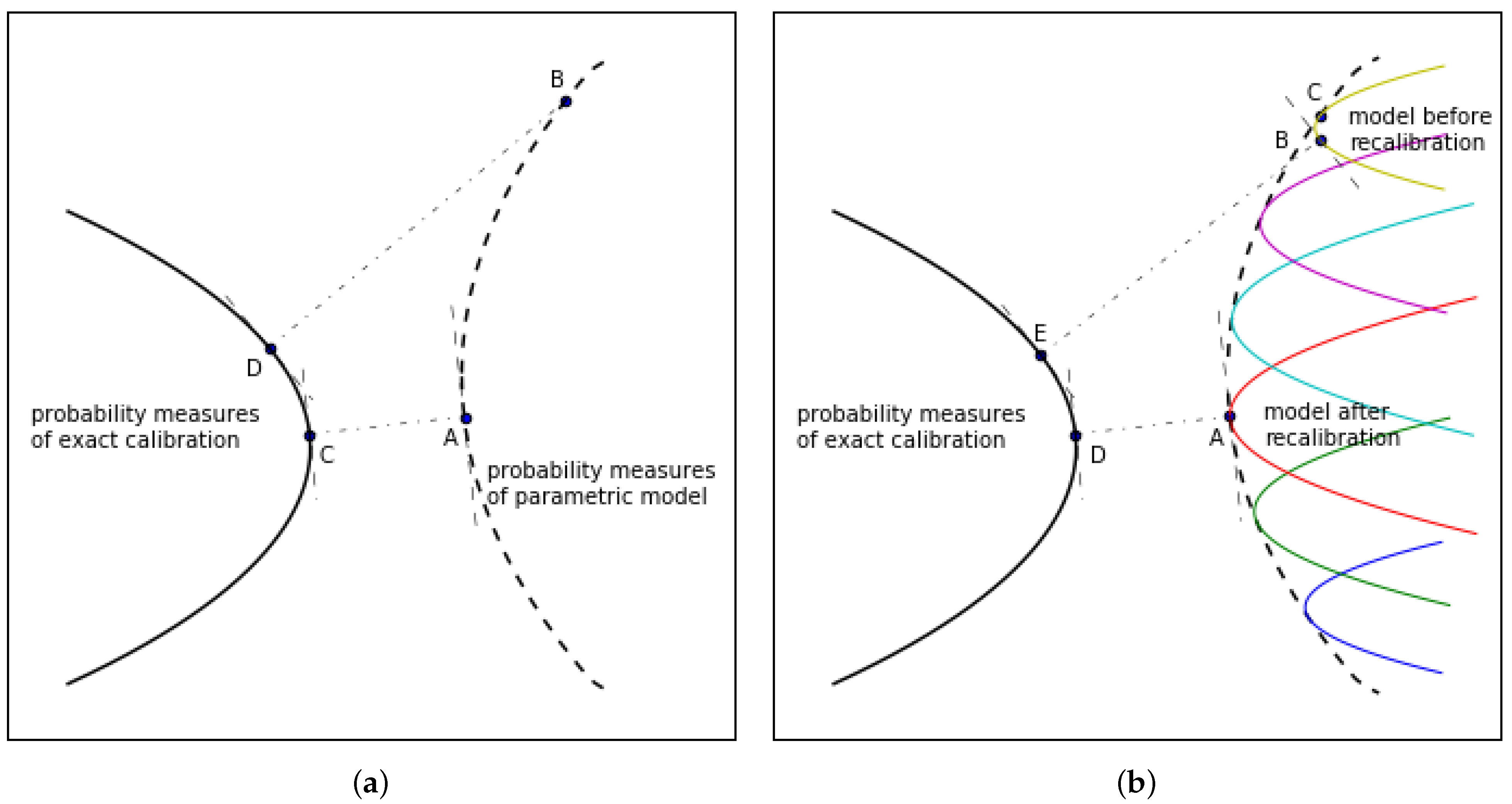
2.1. Quantifying Calibration Error

If we wish to quantify calibration error (Type 1 model risk) in this fashion, then, in Equations (1)–(3), the probability measure P corresponds to the calibrated model and thus is parametric in some form. The probability measure Q, on the other hand, serves as a reference measure exactly matching observed market option prices at a given point in time, unrestricted by the assumptions of the model under consideration. Note that, if we only consider market prices for European options, then these only constrain the risk-neutral distributions Q for a finite number of (discrete) time horizons and, therefore, the requirement (because we are using f-divergence) that Q and P are equivalent measures is not a material restriction—for example, for a fixed time horizon T, the risk-neutral distribution of the underlying asset price implied by a Black and Scholes (1973) model is a probability measure equivalent to the risk–neutral distribution implied by a Heston (1993) stochastic volatility model, because both distributions have a strictly positive density on the same support.
On calibrating an option pricing model, we may regard the measure Q as some non-parametric risk-neutral measure that fits market option prices. However, in practice, the measure Q is not unique, as the market is usually incomplete. For example, based on the result of Breeden and Litzenberger (1978), in order to obtain Q for a single time horizon completely non-parametrically, one would need option prices for a continuum of strikes, which is clearly never available. Therefore, we define the space of all risk-neutral probability measures that fit market prices by S Q S .
We may further define the space of probability measures that are given by all possible choices of parameter values for the target model by S P S . The new calibration methodology that is proposed here aims to minimise the calibration error, as quantified by the divergence between the two measures P and Q, taken from their respective spaces, i.e.,
( Q * , P * ) = arg min Q S Q , P S P D ( Q | | P ) .
This is to say, the new approach attempts to calibrate a model measure P * (i.e., a set of model parameters θ * ) and non-parametric perfect fit to the market (at a given point in time) Q * , in a fashion that minimises the calibration error that is expressed by
η 1 = D ( Q * | | P * ) .
This is not an end in itself—it is required in order to compare model risk due to the calibration error and model risk due to recalibration (as specified in Section 2.2, below) in a unified framework. Here, it is worth reiterating the point that was made in the introduction, that using relative entropy to quantify model risk due to these two sources is motivated by the role of a “relative entropy budget”, as introduced by Glasserman and Xu (2014) in determining worst-case prices or risk measures—i.e., the greater the relative entropy budget, the worse the worst case outcome, with all other things being equal. Furthermore, choosing relative entropy as the divergence pre-metric means that solving (4) corresponds to what Buchen and Kelly (1996) call the “Principle of Minimum Cross-Entropy” for fitting a risk-neutral distribution to market option prices, and given P * , Q * can be obtained in closed form—this is exploited in the numerical implementation in Section 3, below.
The classical approaches of model calibration, such as minimising the mean-squared error between model and market prices for options, would be inappropriate in this context, as they would lead to unnecessarily high model risk quantities. It is the choice of divergence measure that informs the calibration procedure, which results in a pair of probability measures, ( Q * , P * ) , one of which corresponds to the calibrated model while the other provides a consistent reference measure fitting the market exactly.

2.2. Including Model Risk Due to Recalibration

In order to quantify the model risk due to recalibration, let us consider the more specific case where the model is Markovian in a vector of observable state variables X, the model is characterised by a vector of model parameters θ , and market prices are given for European option prices of a single maturity T. This last assumption of a single maturity T avoids the need to constrain the choice of Q in order to ensure the absence of calendar spread arbitrage between non-parametric risk-neutral measures for different time horizons—parametric models typically ensure this by construction. If we appropriately constrain Q, this assumption could be lifted.
Thus, a “model” in our context is a mapping from parameters θ and state variables X at a current time (call it t i ) to a risk-neutral distribution of an underlying asset (or assets) at time horizon T. The two models that are considered below, Black and Scholes (1973) and Heston (1993), both provide such a mapping. Of course, these models also provide more than that, in particular specifying the dynamics of their respective state variables, but that aspect would fall under “Type 3” model risk not considered here.
Suppose that we solved (4) yesterday (at time t i 1 ) to obtain a P * —to be as explicit as possible, denote this by
P t i 1 , X t i 1 ( ω ) , θ t i 1 * ( A ) A F T .
i.e., this is a (conditional) probability measure that is defined on all F T -measurable events, where the conditioning is on the state variables at time t i 1 , X t i 1 , and we write X t i 1 ( ω ) in order to express that the time t i 1 realisations of the state variables are known at the time that these probabilities are evaluated. We write the subscript θ t i 1 * to express that these probabilities are evaluated in a model with parameters that are calibrated by solving (4) at time t i 1 . Furthermore, denote the non-parametric measure Q * that results from solving (4) at time t i 1 by Q t i 1 .
Now, if we recalibrate today (at time t i ) by solving (4), we obtain Q t i and
P t i , X t i ( ω ) , θ t i * ( A ) A F T .
We can then define the model risk quantity due to recalibration, as
η 2 = D ( P t i , X t i ( ω ) , θ t i * | | P t i , X t i ( ω ) , θ t i 1 * ) ,
which is the divergence between the (conditional) probability measures that were evaluated at time t i , where one measure is based on the recalibrated parameters θ t i * and the other is based on the previously calibrated parameters θ t i 1 * (thus, expressing, in terms of divergence, the inconsistency with the model assumptions due to the fact that we are going “outside of the model” to change parameters in recalibration). The aggregate of calibration error and model risk due to recalibration is then
η 3 = D ( Q t i | | P t i , X t i ( ω ) , θ t i 1 * ) ,
i.e., the divergence between the non-parametric probability measure Q t i obtained by solving (4) at time t i , and the non-recalibrated parametric probability measure, consisting of probabilities that are conditional on the state at time t i , but based on model parameters that were obtained by solving (4) at time t i 1 . However, this approach minimises the divergence between the reference distribution and the recalibrated distribution, thus arguably overstating the divergence to the non-recalibrated (i.e., model-consistent) distribution and, therefore, overstating the aggregate model risk η 3 .
Alternatively, we may choose as the non-parametric reference distribution at time t i
Q ^ t i = arg min Q S Q D ( Q | | P t i , X t i ( ω ) , θ t i 1 * ) ,
resulting in a lower aggregate model risk of
η 3 = D ( Q ^ t i | | P t i , X t i ( ω ) , θ t i 1 * ) .
Note that θ t i * is still obtained by solving (4), because both Q t i and Q ^ t i represent non-parametric probability measures that fit observed market prices exactly, so θ t i * remains the best available parametric fit to the market at time t i ( Q ^ t i is only used to determine minimum divergence of the non-recalibrated model to a measure giving a perfect fit).
In the heuristic schematic shown in Figure 1a, point A represents P t i , X t i ( ω ) , θ t i * , being the parametric probability measure “closest” to the set of non-parametric probability measures fitting the market exactly, where point C represents Q t i . If we do not recalibrate at time t i , then we end up with the parametric probability measure P t i , X t i ( ω ) , θ t i 1 * (point B), to which Q ^ t i (point D) is the “closest” non-parametric probability measure fitting the market exactly. Note that these graphs are for the purpose of heuristic illustration only—in particular, we are not requiring that the two sets of probability measures are convex.
In the case of Kullback–Leibler divergence, if Type 1 (calibration error) and 2 (recalibration) model risk involve independent Radon–Nikodym derivatives, then, in the first case considered above, the aggregate model risk equals the sum of the two components. In fact, the Radon–Nikodym derivatives, as random variables, take the key role in evaluating the two types of model risk. At the time the model is recalibrated, we again consider the optimisation (4), with S Q now changed to reflect the change in observed market prices, so we have the following Radon–Nikodym derivatives:
for calibration error : m 1 = d Q t i d P t i , X t i ( ω ) , θ t i *
for model risk due to recalibration : m 2 = d P t i , X t i ( ω ) , θ t i * d P t i , X t i ( ω ) , θ t i 1 *
for aggregate model risk : m 1 m 2 = d Q t i d P t i , X t i ( ω ) , θ t i 1 *
Abbreviating d P t i , X t i ( ω ) , θ t i 1 * as P and d P t i , X t i ( ω ) , θ t i * as P * , the aggregate risk can be expressed in terms of m 1 and m 2 , as
(15) η 3 = E P [ m 1 m 2 ln ( m 1 m 2 ) ] (16) = E P * [ m 1 ln ( m 1 ) ] + E P [ m 1 m 2 ln ( m 2 ) ] (17) = η 1 + [ 1 cov P ( m 1 , m 2 ) ] η 2 + cov P [ m 1 , m 2 ln ( m 2 ) ] .
If m 1 and m 2 are independent, then cov P ( m 2 , m 1 ) = cov P [ m 2 , m 1 ln ( m 1 ) ] = 0 . The total model risk is equal to the sum of the calibration risk and recalibration risk. In our empirical exploration in Section 4, below, we found that this equality is followed quite well by the Black–Scholes model. However, it typically does not hold in the Heston model, suggesting substantial dependence (of Radon–Nikodym derivatives) between the calibration error and model risk due to recalibration. This already foreshadows the clear trade-off between calibration error and model risk, due to recalibration in the model that is better able to calibrate to option prices across different strikes (i.e., the Heston model) due to its larger number of parameters. If this greater freedom to fit the market reduces calibration error, but effectively only pushes the model risk from Type 1 to Type 2, this dependence between m 1 and m 2 is to be expected.

2.3. The Treatment of Latent State Variables

A model may also involve one or more latent state variables. An example of that is the class of stochastic volatility models where the volatility is taken as a latent state variable, rather than a model parameter (in the empirical examples in Section 4 below, we specifically consider the model of Heston (1993), which falls into this category). Under the framework of a single stochastic volatility state variable, a model that is specified by a given set of parameters forms a one-dimensional manifold (Figure 1b) for possible realisations of the state variable, rather than a point in the Black/Scholes world (Figure 1a).
Thus, the model that we are now considering is Markovian in a vector of state variables ( X , V ) , where the state variables X are observable and the state variables V are latent (unobservable). Subsequently, the initial calibration problem (4) becomes
( Q * , v * , θ * ) = arg min Q S Q , v S v , θ S θ D ( Q | | P ( v ; θ ) ) ,
where S v and S θ are the sets of legitimate values of the state variables and the parameters, respectively. θ * is the set of model parameters calibrated to the market, and v * is the best estimate of the latent state variables under the calibrated model. This effectively treats the latent (unobserved) state variable as an additional parameter to be calibrated, but the recalibration of which does not contribute to (Type 2) model risk, due to recalibration, because it is consistent with the model assumptions for this latent state variable to evolve stochastically. This does shift Type 2 model risk to Type 3, the risk that the state variable dynamics are not (econometrically) consistent with the dynamics that are assumed in the model. However, in the present paper, we deliberately set aside Type 3 model risk for the purposes of our analysis, leaving the integration of all four types of model risk for future research.
The notation in (6) is amended to
P t i 1 , X t i 1 ( ω ) , v t i 1 * , θ t i 1 * ( A ) A F T .
At time t i , we have, for the calibration error,
η 1 = D ( Q t i | | P t i , X t i ( ω ) , v t i * , θ t i * ) .
The model risk due to recalibration is
η 2 = D ( P t i , X t i ( ω ) , v t i * , θ t i * | | P t i , X t i ( ω ) , v t i * , θ t i 1 * ) .
The aggregate model risk while using Q t i from Q * and v t i * from v * in (18) is
η 3 = D ( Q t i | | P t i , X t i ( ω ) , v t i * , θ t i 1 * )
or, alternatively, using Q ^ t i and v ^ t i determined analogously to (10), i.e.,
( Q ^ t i , v ^ t i ) = arg min Q S Q , v S v D ( Q | | P t i , X t i ( ω ) , v , θ t i 1 * ) ,
which results in
η ^ 3 = D ( Q ^ t i | | P t i , X t i ( ω ) , v ^ t i , θ t i 1 * ) .
We then have the following Radon–Nikodym derivatives:
for calibration error : m 1 = d Q t i d P t i , X t i ( ω ) , v t i * , θ t i *
for model risk due to recalibration : m 2 = d P t i , X t i ( ω ) , v t i * , θ t i * d P t i , X t i ( ω ) , v t i * , θ t i 1 *
for aggregate model risk : m 1 m 2 = d Q t i d P t i , X t i ( ω ) , v t i * , θ t i 1 *
Note that the key difference between (12)–(14) and (25)–(27) is that the change in v, being permitted by the model assumptions, does not contribute to the model risk quantities. In (4) and (18), we are deliberately prioritising the minimisation of calibration error, as this is congruent to the (often exclusive) focus of practitioners on calibration error (with little or no regard to model risk due to recalibration). If desired, one could reformulate this approach in order to prioritise the minimisation of aggregate model risk or of model risk due to recalibration.

3. Numerical Implementation

In this section, we outline the numerical scheme for solving the minimisation problems that arise when taking into account calibration error and model risk, due to recalibration in the manner that is described in the previous section, including problems of the type (4) involving the optimal choice of two probability measures. In this case, an iterative process is required, optimising two probability measures Q and P, in turn, until convergence, in the following manner:
(1)
Produce P ( 0 ) from a parametric model that is based on an initial guess of the model parameters (and latent state variables, where required).
(2)
Solve, for Q ( 0 ) , via Lagrange multipliers for the constrained problem that minimises D ( Q ( 0 ) | | P ( 0 ) ) .
(3)
Solve, for P ( 1 ) , to obtain model parameters for the P ( 1 ) that minimises D ( Q ( 0 ) | | P ( 1 ) ) .
(4)
Iterate steps 2 and 3: P ( n ) Q ( n ) P ( n + 1 ) until convergence.

3.1. Step 1

In Step 1, the initial guess may be obtained in several different ways. A common way is to minimise the mean-squared error between model and market option prices at all available strikes (see e.g., Cui et al. (2017)). We opted for the Broyden/Fletcher/Goldfarb/ Shanno (BFGS) algorithm for conducting this initial calibration of the model parameters and (where required) latent state variables. In practice, the particular choice of the initial guess in Step 1 appears to have little impact in our implementation, as Step 4 converged quite quickly.

3.2. Step 2

In Step 2, we solve the following constrained minimisation problem whlie using Lagrange multipliers:
Q ( 0 ) = arg min Q S Q D ( Q | | P ( 0 ) )
s . t . B E Q ( Z ) A .
Note that, here, we specify the constraints in the form of expectations under the measure Q, where these expectation are the model prices for our calibration instruments for the model that is based on the non-parametric reference distribution Q. In general, B , Z , and A are vectors; thus, (29) is a “stack” of inequality constraints representing observed market prices. Additionally, notice that, for generality, we “relax” each equality constraint into two inequality constraints. This is in order to account for the bid-ask spread of each option traded on the market. The vector B denotes a list of bid prices, while the vector A contains ask prices. In a simplified scenario, where exact option prices are given, we may set B = A . Z denotes the vector of discounted option payoffs. By introducing vectors of Lagrange multipliers λ B and λ A , we convert the constrained problem to an unconstrained dual problem,
max λ B 0 , λ A 0 min Q S Q D ( Q | | P ( 0 ) ) λ B E Q ( Z ) B λ A E Q ( Z ) A .
In the case of Kullback–Leibler divergence, solving the inner problem corresponds to the “Principle of Minimum Cross-Entropy” in Buchen and Kelly (1996). By Equation (11) in that paper, the probability density function q ( 0 ) of Q ( 0 ) is given in terms of the density p ( 0 ) of P ( 0 ) , by
q ( 0 ) = p ( 0 ) e λ Z E P ( 0 ) e λ Z .
Note that
D ( Q ( 0 ) | | P ( 0 ) ) = Ω d Q ( 0 ) d P ( 0 ) ln d Q ( 0 ) d P ( 0 ) d P ( 0 ) = Ω ln d Q ( 0 ) d P ( 0 ) d Q ( 0 ) = E Q ( 0 ) ln d Q ( 0 ) d P ( 0 )
and (31) implies
d Q ( 0 ) d P ( 0 ) = q ( 0 ) p ( 0 ) = e λ Z E P ( 0 ) e λ Z .
Substituting (31) into (30), we obtain a maximisation problem,
max λ B 0 , λ A 0 E Q ( 0 ) ( λ B + λ A ) Z ln E P ( 0 ) e ( λ B + λ A ) Z
λ B E Q ( Z ) B λ A E Q ( Z ) A
= max λ B 0 , λ A 0 ln E P ( 0 ) e ( λ B + λ A ) Z + λ B B + λ A A
= max λ B 0 , λ A 0 ln E P ( 0 ) e ( λ B + λ A ) Z + ( λ B + λ A ) B + A 2 ( λ B λ A ) A B 2 .
If B = A , then the last term vanishes, representing the problem with exact market prices. If (component-wise) B > A , then the last term reflects a penality on the objective function that is proportional to the difference of the two Lagrange multipliers. Therefore, we may transform the Lagrange multipliers by
λ + = λ B + λ A
λ = λ B λ A
and the objective function becomes
max λ + R d , λ | λ + | ln E P ( 0 ) e λ + Z + λ + B + A 2 λ A B 2 .
Because λ only appears in the final, negative term, maximising (39) implies that λ must be as small as possible, so we can set λ = | λ + | , and the objective function becomes
max λ + R d ln E P ( 0 ) e λ + Z + λ + B + A 2 | λ + | A B 2 .
We can numerically solve the maximization problem by taking its gradient with respect to λ + ,
E P ( 0 ) Z e λ + Z = B + A 2 sgn ( λ + ) A B 2 E P ( 0 ) e λ + Z ,
where the element-wise sign function sgn ( λ + ) assigns 1, −1, or 0 to each element of λ + . However, due to the discontinuouity of the sign, function (41) cannot be solved directly in a stable way. In order to bypass this problem, we approximate the sign function with a continuous step function:
sgn ( x ) = 1 2 1 + exp x δ .
We use Powell’s hybrid method in order to solve the multidimensional Equations (41), where δ controls the steepness of the function and choosing this value is critical for a fast and stable convergence of the method, i.e., with a careful choice of δ , Step 2 converges quickly.

3.3. Steps 3 and 4

In Step 3, we use the L-BFGS-B algorithm to minimise the divergence with respect to model parameters (or latent variables or both). This step corresponds to the quite standard process of calibrating a parametric option pricing model, and it does not result in any difficulties in obtaining convergence. Step 2 and Step 3 are repeated until convergence. The convergence criterion that is adopted here is that all of the percentage changes of parameters after one iteration do not exceed a certain threshold, say 0.1%. On this “outer” convergence, in practice we did not encounter any difficulties either, which may be due to the convexity of the sets constraining P and Q.

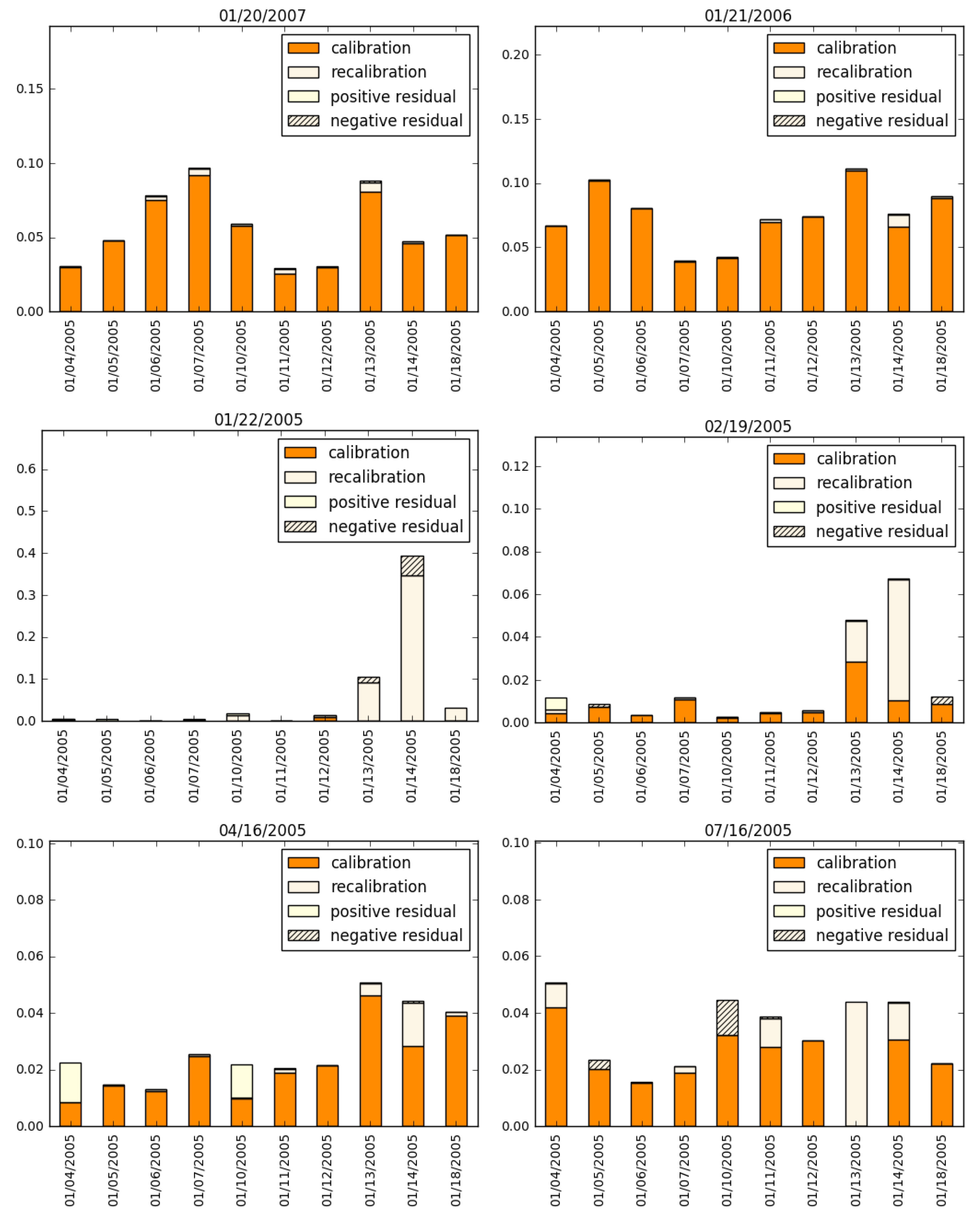
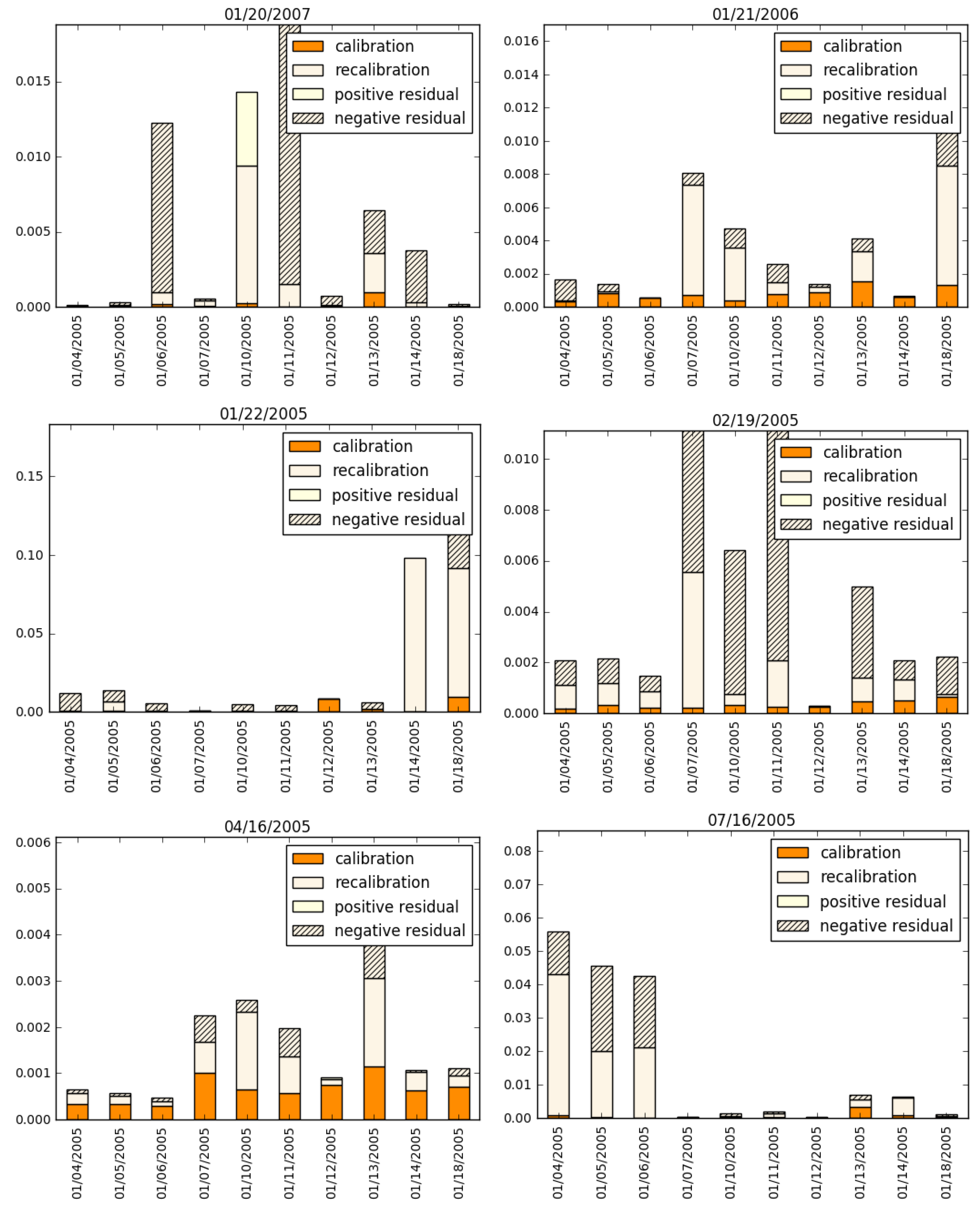
4. Examining the Trade-Off between Calibration Error and Model Risk Due to Recalibration

As an application example of the method that is described in the previous two sections, we consider historical data that consist of daily market prices for call options on Apple (AAPL) and Google (GOOG) stock over a period from 6 January 2004 to 19 December 2008 for AAPL and 4 January 2005 to 19 December 2008 for GOOG. This gives us a reasonably straightforward application example that is free of extraneous complications, while still reasonably covering liquid options and including a period of “interesting” market volatility (August 2007): although these options are of the American type, i.e., permitting early exercise, AAPL and GOOG did not pay any dividends during this period. Thus, the possibility of early exercise may be ignored (see Merton (1973)).
From these data, we remove options that are very far away from the money, restricting the range of strikes from delta 2.5% to delta 97.5%. Furthermore, we remove prices of options that had zero trading volume on a given day, in order to avoid using prices that are likely to be stale.
On these data, we consider two parametric models, Black and Scholes (1973) and Heston (1993)—arguably the two most popular option pricing models available, where the latter introduces a latent variable for stochastic volatility. The unified methodology, quantifying calibration error, model risk due to recalibration, and the aggregate of the two allows for us to explore the trade-off between calibration error (which is, unsurprisingly, reduced by moving from Black and Scholes (1973) to Heston (1993)) and model risk due to recalibration (which has hitherto been largely ignored) when moving from one parametric model to another, as well as when changing the frequency with which the model is recalibrated.
We start by evaluating the calibration, recalibration, and aggregated model risk quantities under a Black/Scholes model, i.e., where the underlying asset price is assumed to follow geometric Brownian motion, with dynamics under the risk-neutral measure that is given by
d S ( t ) = r S ( t ) d t + σ S ( t ) d W ( t ) ,
where r is the continuously compounded risk-free rate of interest and σ is a constant volatility parameter. In Appendix A, we note that, in the Black/Scholes model, we obtain a simple closed form expression for the recalibration model risk quantity that is defined in (8):
η 2 = σ * 2 σ 2 1 1 2 + T 8 ( σ * 2 σ 2 ) + ln σ σ * ,
where σ * is the correctly recalibrated Black/Scholes volatility parameter and σ is the parameter value that was obtained in a previous calibration. This formula is a consequence of the log-normal distribution of returns assumed in the Black/Scholes model.
We can express the aggregate model risk as the sum of the calibration error, the recalibration risk, and a residual. The residual is zero if the likelihood ratios that are involved in the calibration and recalibration risks are two independent random variables, as noted in Equation (15). In practice, the residual usually takes a small non-zero value. In Figure 2, we demonstrate the decomposition of the total model risk into the three components. Unsurprisingly (as it is well documented that the Black/Scholes model cannot fit the implied volatility “smile” observed in most options markets), we see that calibration error typically predominates.
In the Heston model, the dynamics (43) are extended in order to allow for stochastic volatility, i.e.,
d S ( t ) = r S ( t ) d t + σ ( t ) S ( t ) d W 1 ( t )
d ( σ 2 ( t ) ) = κ ( θ σ 2 ( t ) ) d t + η σ ( t ) d W 2 ( t ) .
This model involves two state variables, the underlying asset price S ( t ) and the volatility σ ( t ) , and five model parameters: r, κ , θ , η , and ρ , where ρ is the correlation coefficient between the two Wiener processes:
d W 1 , W 2 t = ρ d t .
r is the risk-free rate, and κ , θ and η relate to the volatility process, with κ being the rate of mean reversion, θ the long-run mean, and η the volatility of this process.
In our empirical application examples, we take the risk-free rate as one of the financial variables that were observed in the market, but we do not explicitly take the interest rate risk in our empirical analysis into account. For the short-dated options that were considered here, interest rate risk is known to be of relatively little importance—for a discussion of this issue, see e.g., Cheng et al. (2018) and the literature cited therein.
Following Gatheral (2006), Equation (2.13), the risk-neutral probability of exercise of a European call option with strike K in the Heston model is given by
P 0 ( x , v , τ ) = 1 2 + 1 π 0 R exp { C ( u , τ ) θ + D ( u , τ ) v + i u x } i u d u ,
where v is the current value of the volatility state variable σ ( t ) , τ = T t is the time to maturity, and x is the logarithmic forward moneyness of the option, i.e.,
x : = ln F t , T K F t , T = S ( t ) B ( t , T )
with B ( t , T ) the time t price of a zero bond maturing in T. Furthermore,
C ( u , τ ) = κ r τ 2 η 2 ln r + r e d τ r + r
D ( u , τ ) = r r + r + e d τ r + r e d τ
r ± = β ± d η 2 d = β 2 2 α η 2 .
Parameters α and β are functions of u (Fourier transform variable of x):
α ( u ) = u 2 2 i u 2
β ( u ) = κ ρ η i u .
It is noted that P 0 = E Q ( 1 S T > K ) , since, by definition, P 0 is the probability of exercise. Therefore, the probability density function of the risk-neutral measure is obtained:
(53) p ( S T ) = P 0 K K = S T = P 0 x x K K = S T (54) = 1 2 π S T R exp C ( u , τ ) θ + D ( u , τ ) v + i u ln S t B ( t , T ) S T d u .
For simplicity, e y denotes the ratio of the forward price at t to its spot price at maturity T, i.e., e y = B ( t , T ) S T / S t , we derive the risk-neutral probability with respect to y:
p ( y ) = p ( S T ) y S T 1
= 1 2 π R exp C ( u , τ ) θ + D ( u , τ ) v i u y d u .
p ( y ) can be calculated by fast Fourier transform (FFT). We use this in each step of our iterative procedure, where a risk-neutral probability measure P as a function of the model parameters and state variables is required for the Heston model, i.e., when fitting an initial guess of the model parameters to market option prices in Step 1, when using P ( 0 ) in Step 2, when solving for P ( 1 ) in Step 3, and so on.
The decomposition of the total model risk into the three components (the components due to calibration and recalibration, and the positive or negative residual measuring the departure from independence between the first two components) when using the Heston model as the baseline is given in Figure 3. Again, because it is well documented that the Heston model can fit observed option prices better than Black/Scholes, it is unsurprising that, in this case, the relative entropy measuring calibration error is much lower—however, already in this set of example days, it is evident that this comes at the price of increased model risk due to recalibration.
These observations are reinforced when we consider aggregate model risk, calibration error, and model risk due to recalibration over the entire sample period, as presented in Table 1 and Table 2. Note that the absolute numbers refer to relative entropy and, thus, lack direct financial interpretation—what matters are the relative values when comparing the model across models and different recalibration frequencies, in particular when considering the aggregate model risk. Here, we consider recalibrating the Black/Scholes and Heston models either daily, every three days, every week, every two weeks, or every quarter year. Thus, for each model and each recalibration frequency, we get a (for example, daily) sequence of model risk quantities for each of the three types (calibration, recalibration, and aggregate). In each column, we report summary statistics of such a sequence, i.e., its mean, median, and the 99%, 95%, 90%, and 75% quantiles. Note that on days on which we do not recalibrate, the model risk, due to recalibration being zero, because (consistent with the model assumptions) we are keeping previously calibrated parameters unchanged—so, on those days, aggregate model risk is entirely due to calibration error (which increases because the fit to market prices deteriorates when we do not recalibrate).
We see that recalibrating more frequently has little effect on the aggregate model risk, neither when using the Black/Scholes model nor when using the Heston model. Essentially, recalibrating more frequently simply shifts calibration error into model risk, due to recalibration, highlighting the dangers in the common practice of focusing solely on the calibration of derivative pricing models, at the expense of all other sources of model risk.
In addition, we observe that if we are interested in “robustness” at a high level of confidence (looking at, say, the 99% quantile of aggregate model risk), moving from Black/Scholes to Heston also does not appear to deliver any advantage (it does yield some improvement at lower quantiles, or average or median, aggregate model risk). This means that, when high levels of confidence are required, any gain in calibration accuracy that is delivered by the Heston model is offset by higher model risk due to recalibration. One should note that this last point holds, even before considering Type 3 model risk, which may well be worse when additional state variables are introduced (as in the Heston model). For these results, in Table 1 and Table 2, we calculated the means, medians, and quantiles across all available option maturities. If we only consider particular maturity “buckets” (i.e., considering only subsets of options, with maturities in a particular range), the same qualitative conclusions are evident—Table 3 and Table 4 illustrate this in the case of daily recalibration.

5. Conclusions

Under our approach, less relative entropy implies less model risk, and we are able to evaluate two hitherto disparate sources of model risk (calibration error and model risk due to recalibration) in a unified fashion, and examine the potential trade-off between the two. We have considered a simple choice between two models, and between different recalibration frequencies. “Putting a number on model risk” by calculating quantiles for the maximum model risk (quantified by relative entropy) over a time series of market data allows for one to assess the added value (if any) of more complicated stochastic models of financial markets.
One should note that, instead of using a relative entropy pre-metric, one could approach quantifying model risk in terms of optimal-transport distance, while using for example Wasserstein distance, which most recently has become popular for this purpose (see Bartl et al. (2020); Blanchet et al. (2018) and Feng and Schlögl (2018)). In the present paper, we have followed the more established approach while using relative entropy, which, in economics, has its roots in the seminal work of Hansen and Sargent (see e.g., Hansen and Sargent (2006)), as well as a long history of application in other fields, such as thermodynamics and information theory.
In our application, we are deliberately prioritising the minimisation of calibration error, as this is congruent to the (often exclusive) focus of practitioners on calibration error (with little or no regard to model risk due to recalibration). Even in this case, we see that, by including recalibration as one of the sources of aggregate model risk, frequently recalibrating a model to a changing market simply interchanges one source of model risk for another, and more complicated stochastic models may well underperform when aggregate model risk is taken into account.

Author Contributions

Conceptualisation, Y.F. and E.S.; Formal analysis, Y.F.; Investigation, Y.F., R.R., C.B., Q.M. and M.M.; Methodology, Y.F. and E.S.; Resources, E.S.; Software, Y.F.; Supervision, E.S.; Visualisation, Y.F.; Writing-original draft, Y.F. and E.S.; Writing-review & editing, E.S. All authors have read and agreed to the published version of the manuscript.

Funding

This research received no external funding.

Institutional Review Board Statement

Not applicable.

Informed Consent Statement

Not applicable.

Data Availability Statement

Data was obtained from IVolatility and are available via https://www.ivolatility.com/data/historical_data2.html.

Acknowledgments

Part of the initial research for this paper was conducted at the Financial Mathematics Team Challenge 2016 at the University of Cape Town. We would like to thank Sam Cohen and Hardy Hulley for helpful comments on earlier drafts of this paper. The usual disclaimers apply.

Conflicts of Interest

The authors declare no conflict of interest.

Appendix A. Derivation of the Recalibration Model Risk Quantity in the Black/Scholes Model

Denote by g σ ( S T | S 0 ) the risk–neutral probability density of the stock price at time T given the stock price at time 0, in a Black and Scholes (1973) model with volatility σ . This is given by
g σ ( S T | S 0 ) = 1 S T σ 2 π exp ( ln S T ln S 0 r T + 1 2 σ 2 T ) 2 2 σ 2 T .
Furthermore, denote by σ * the correctly recalibrated Black/Scholes volatility parameter and by σ the parameter value obtained in a previous calibration. The model risk quantity due to recalibration defined in (8) then becomes
(A2) η 2 = 0 g σ * ( S T | S 0 ) g σ ( S T | S 0 ) ln g σ * ( S T | S 0 ) g σ ( S T | S 0 ) g σ ( S T | S 0 ) d S T (A3) = 0 ln g σ * ( S T | S 0 ) g σ ( S T | S 0 ) g σ * ( S T | S 0 ) d S T .
Therefore,
η 2 = 0 ( ( ln S T ln S 0 r T + 1 2 σ 2 T ) 2 2 σ 2 T ( ln S T ln S 0 r T + 1 2 σ * 2 T ) 2 2 σ * 2 T + ln ( S T σ 2 π ) ln ( S T σ * 2 π ) ) g σ * ( S T | S 0 ) d S T .
Consider the different parts (A4) in turn:
(A5) 0 ( ln ( S T σ 2 π ) ln ( S T σ * 2 π ) g σ * ( S T | S 0 ) d S T = ln σ σ * (A6) 0 ( ln S T ln S 0 r T + 1 2 σ * 2 T ) 2 2 σ * 2 T g σ * ( S T | S 0 ) d S T = Var [ ln S T ] 2 σ * 2 T = 1 2
and
(A7) 0 ( ln S T ln S 0 r T + 1 2 σ 2 T ) 2 2 σ 2 T g σ * ( S T | S 0 ) d S T = 1 2 σ 2 T 0 ( ln S T ln S 0 r T + 1 2 σ * 2 T 2 + 2 ( ln S T ln S 0 r T ) 1 2 σ * 2 T (A8) 2 ( ln S T ln S 0 r T ) 1 2 σ 2 T 1 4 σ * 4 T 2 + 1 4 σ 4 T 2 ) g σ * ( S T | S 0 ) d S T (A9) = 1 2 σ 2 T σ * 2 T σ * 2 T 1 2 σ * 2 T + σ 2 T 1 2 σ * 2 T 1 4 σ * 4 T 2 + 1 4 σ 4 T 2 (A10) = σ * 2 2 σ 2 + T 8 σ * 4 σ 2 2 σ * 2 + σ 2 .
Combining (A5), (A6) and (A10) gives
η 2 = σ * 2 σ 2 1 1 2 + T 8 ( σ * 2 σ 2 ) + ln σ σ * .

References

  1. Ahmadi-Javid, Amir. 2012. Entropic value-at-risk: A new coherent risk measure. Journal of Optimization Theory and Applications 155: 1105–23. [Google Scholar] [CrossRef]
  2. Ali, Syed Mumtaz, and Samuel D. Silvey. 1966. A general class of coefficients of divergence of one distribution from another. Journal of the Royal Statistical Society: Series B 28: 131–42. [Google Scholar] [CrossRef]
  3. Bannör, Karl F., and Matthias Scherer. 2013. Capturing parameter risk with convex risk measures. European Actuarial Journal 3: 97–132. [Google Scholar] [CrossRef]
  4. Bartl, Daniel, Samuel Drapeau, and Ludovic Tangpi. 2020. Computational aspects of robust optimized certainty equivalents and option pricing. Mathematical Finance 30: 287–309. [Google Scholar] [CrossRef] [Green Version]
  5. Black, Fischer, and Myron Scholes. 1973. The pricing of options and corporate liabilities. Journal of Political Economy 81: 637–54. [Google Scholar] [CrossRef] [Green Version]
  6. Blanchet, Jose, Lin Chen, and Xun Yu Zhou. 2018. Distributionally robust mean–variance portfolio selection withWasserstein distances. arXiv, arXiv:1802.04885. [Google Scholar]
  7. Board of Governors of the Federal Reserve System Office of the Comptroller of the Currency. 2011. Supervisory Guidance on Model Risk Management. Technical Report OCC 2011-12 Attachment. Washington D.C.: Office of the Comptroller of the Currency. [Google Scholar]
  8. Boucher, Christophe M., Jón Danielsson, Patrick S. Kouontchou, and Bertrand B. Maillet. 2014. Risk models–at–risk. Journal of Banking & Finance 44: 72–92. [Google Scholar]
  9. Box, George E. P., and Norman R. Draper. 1987. Empirical Model–Building and Response Surfaces. Hoboken: Wiley. [Google Scholar]
  10. Breeden, Douglas T., and Robert H. Litzenberger. 1978. Prices of state-contingent claims implicit in option prices. Journal of Business 51: 621–51. [Google Scholar] [CrossRef]
  11. Breuer, Thomas, and Imre Csiszár. 2016. Measuring distribution model risk. Mathematical Finance 26: 395–411. [Google Scholar] [CrossRef] [Green Version]
  12. Buchen, Peter W., and Michael Kelly. 1996. The maximum entropy distribution of an asset inferred from option prices. Journal of Financial and Quantitative Analysis 31: 143–59. [Google Scholar] [CrossRef]
  13. Cheng, Benjamin, Christina Sklibosios Nikitopoulos, and Erik Schlögl. 2018. Pricing of long-dated commodity derivatives: Do stochastic interest rates matter? Journal of Banking & Finance 95: 148–66. [Google Scholar]
  14. Csiszár, Imre. 1967. Information-type measures of difference of probability distributions and indirect observations. Studia Scientiarum Mathematicarum Hungarica 2: 299–318. [Google Scholar]
  15. Cui, Yiran, Sebastian del Baño Rollin, and Guido Germano. 2017. Full and fast calibration of the Heston stochastic volatility model. European Journal of Operational Research 263: 625–38. [Google Scholar] [CrossRef]
  16. Detering, Nils, and Natalie Packham. 2016. Model risk of contingent claims. Quantitative Finance 16: 1357–74. [Google Scholar] [CrossRef]
  17. Feng, Yu, and Erik Schlögl. 2018. Model risk measurement under Wasserstein distance. arXiv, arXiv:1809.03641. [Google Scholar] [CrossRef] [Green Version]
  18. Gatheral, Jim. 2006. The Volatility Surface: A Practitioner’s Guide. Hoboken: John Wiley & Sons. [Google Scholar]
  19. Glasserman, Paul, and Xingbo Xu. 2014. Robust risk measurement and model risk. Quantitative Finance 14: 29–58. [Google Scholar] [CrossRef]
  20. Hansen, Lars Peter, and Thomas J. Sargent. 2006. Robustness. Princeton: Princeton University Press. [Google Scholar]
  21. Heston, Steven L. 1993. A closed–form solution for options with stochastic volatility with applications to bond and currency options. The Review of Financial Studies 6: 327–43. [Google Scholar] [CrossRef] [Green Version]
  22. Kerkhof, Jeroen, Bertrand Melenberg, and Hans Schumacher. 2010. Model risk and capital reserves. Journal of Banking & Finance 34: 267–79. [Google Scholar]
  23. Löffler, Gunter. 2003. The effects of estimation error on measures of portfolio credit risk. Journal of Banking & Finance 27: 1427–53. [Google Scholar]
  24. Merton, Robert C. 1973. Theory of rational option pricing. The Bell Journal of Economics and Management Science 4: 141–83. [Google Scholar] [CrossRef] [Green Version]
Figure 1. Graphic illustration of the mathematical definitions of model risks for (a) observable state variable, (b) latent state variable.
Risks 09 00013 g001
Figure 2. Decomposition of model risks of Apple (AAPL) options while using the Black/Scholes model as the nominal model, for a selection of option maturity dates (given as the title of each graph). The vertical axis denotes the numerical value of the relative entropy.
Risks 09 00013 g002
Figure 3. Decomposition of model risks of Google (GOOG) options while using the Heston model as the nominal model, for a selection of option maturity dates (given as the title of each graph). The vertical axis denotes the numerical value of the relative entropy.
Risks 09 00013 g003
Table 1. Model risks (in terms of relative entropy) under different models and recalibration frequencies for AAPL.
Risk MeasureBlack-ScholesHeston
1 Day3 Days1 Week2 Weeks1 Quarter1 Day3 Days1 Week2 Weeks1 Quarter
Aggregate Model Risk
mean0.0700.0710.0730.0730.0850.0370.0350.0380.0390.046
median0.0450.0470.0470.0510.0570.0050.0050.0050.0060.010
Quantile99%0.4740.4270.4710.4550.4620.5080.4620.5120.5030.649
95%0.2120.2210.2210.2120.2510.1730.1690.1770.1770.185
90%0.1580.1600.1650.1600.1920.0960.0970.0980.1050.121
75%0.0920.0940.0950.0990.1120.0270.0270.0290.0310.034
Calibration Error
mean0.0550.0660.0690.0720.0840.0080.0260.0320.0360.045
median0.0380.0430.0450.0490.0570.0010.0030.0040.0050.009
Quantile99%0.2390.3970.4330.4430.4550.1630.4160.4960.4950.648
95%0.1710.2070.2120.2100.2490.0150.1300.1580.1680.182
90%0.1350.1510.1580.1580.1910.0080.0650.0830.0970.119
75%0.0750.0870.0910.0960.1110.0030.0120.0190.0260.034
Model Risk due to Recalibration
mean0.0240.0090.0050.0020.0010.0570.0190.0110.0060.001
median0.0020.0010.0010.0000.0000.0040.0010.0010.0010.000
Quantile99%0.4580.1960.0570.0300.0120.6300.2260.1170.0670.011
95%0.1030.0340.0210.0100.0050.3150.1080.0620.0320.006
90%0.0560.0200.0110.0060.0020.1640.0520.0310.0160.004
75%0.0130.0060.0040.0020.0010.0550.0160.0110.0050.001
Table 2. Model risks (in terms of relative entropy) under different models and recalibration frequencies for GOOG.
Risk MeasureBlack-ScholesHeston
1 Day3 Days1 Week2 Weeks1 Quarter1 Day3 Days1 Week2 Weeks1 Quarter
Aggregate Model Risk
mean0.1650.1680.1650.1650.1880.1150.1050.1130.1140.127
median0.1090.1110.1120.1150.1380.0530.0500.0550.0530.059
Quantile99%0.7050.7220.7220.6990.7280.7260.6680.7110.6990.744
95%0.5190.5300.5210.4960.5490.4750.4380.4550.4670.560
90%0.3930.3910.3870.3850.4080.3300.2870.3200.3240.380
75%0.2190.2230.2140.2150.2560.1450.1370.1420.1530.157
Calibration Error
mean0.1250.1550.1580.1620.1870.0550.0830.1030.1070.126
median0.0820.1020.1060.1110.1370.0060.0220.0430.0460.058
Quantile99%0.6550.7010.7090.6960.7280.6260.6510.7060.6880.744
95%0.4000.4820.5070.4940.5480.3290.3810.4380.4450.557
90%0.2950.3590.3620.3790.4080.1720.2500.2980.3060.375
75%0.1710.2080.2070.2120.2550.0340.1030.1270.1410.155
Model Risk due to Recalibration
mean0.0360.0140.0080.0040.0010.1190.0440.0120.0120.003
median0.0040.0020.0010.0010.0000.0430.0160.0030.0030.001
Quantile99%0.4050.1720.0910.0500.0100.7570.2550.0870.0770.012
95%0.1730.0660.0350.0180.0040.5430.1870.0560.0640.011
90%0.1090.0380.0220.0120.0030.4110.1510.0340.0450.009
75%0.0360.0130.0080.0040.0010.1420.0520.0160.0130.003
Table 3. Model risks (in terms of relative entropy) under different models, by maturity buckets, for AAPL (daily recalibration frequency).
Risk MeasureBlack-ScholesHeston
All0–0.2 Year0.2–0.7 Year>0.7 YearAll0–0.2 Year0.2–0.7 Year>0.7 Year
Aggregate Model Risk
mean0.0700.0410.0660.1090.0370.0390.0240.046
median0.0450.0210.0520.0810.0050.0040.0040.008
Quantile99%0.4740.4710.2660.5670.5080.5900.3020.472
95%0.2120.1200.1850.2820.1730.2430.0910.191
90%0.1580.0810.1430.2130.0960.0740.0660.142
75%0.0920.0470.0900.1410.0270.0210.0150.054
Calibration Error
mean0.0550.0260.0570.0870.0080.0120.0040.007
median0.0380.0140.0480.0680.0010.0010.0010.001
Quantile99%0.2390.1570.2300.2890.1630.0720.0520.116
95%0.1710.0910.1570.2120.0150.0210.0110.017
90%0.1350.0620.1260.1810.0080.0060.0070.010
75%0.0750.0360.0770.1280.0030.0020.0030.003
Model Risk due to Recalibration
mean0.0240.0200.0130.0380.0570.0620.0480.060
median0.0020.0020.0010.0030.0040.0040.0030.009
Quantile99%0.4580.5060.1160.6620.6300.7020.5360.512
95%0.1030.0660.0660.1690.3150.4430.2740.247
90%0.0560.0300.0420.1020.1640.2230.1270.160
75%0.0130.0090.0100.0310.0550.0300.0480.091
Table 4. Model risks (in terms of relative entropy) under different models, by maturity buckets, for GOOG (daily recalibration frequency).
Risk MeasureBlack-ScholesHeston
All0–0.2 Year0.2–0.7 Year>0.7 YearAll0–0.2 Year0.2–0.7 Year>0.7 Year
Aggregate Model Risk
mean0.1650.1670.1620.1640.1150.1150.1200.109
median0.1090.1040.0990.1200.0530.0520.0570.048
Quantile99%0.7050.7360.7090.6610.7260.7140.7070.736
95%0.5190.5270.5510.4590.4750.4680.5000.476
90%0.3930.4170.3820.3710.3300.3510.3220.304
75%0.2190.2210.2160.2180.1450.1490.1550.136
Calibration Error
mean0.1250.1210.1230.1320.0550.0550.0520.057
median0.0820.0740.0750.0990.0060.0050.0060.006
Quantile99%0.6550.6620.6500.6390.6260.6580.5310.665
95%0.4000.4030.4230.3910.3290.3490.3110.330
90%0.2950.2980.3010.2850.1720.1550.1850.171
75%0.1710.1620.1600.1760.0340.0310.0340.034
Model Risk due to Recalibration
mean0.0360.0380.0390.0330.1190.1170.1170.124
median0.0040.0050.0030.0050.0430.0430.0370.049
Quantile99%0.4050.4190.4790.2840.7570.7460.7670.754
95%0.1730.1760.1880.1550.5430.5100.5580.554
90%0.1090.1110.1150.0980.4110.3900.4180.418
75%0.0360.0380.0320.0360.1420.1440.1370.146
Publisher’s Note: MDPI stays neutral with regard to jurisdictional claims in published maps and institutional affiliations.

