Retrospective Reserves and Bonus with Policyholder Behavior

Abstract

Legislation imposes insurance companies to project their assets and liabilities in various financial scenarios. Within the setup of with-profit life insurance, we consider retrospective reserves and bonus, and we study projection of balances with and without policyholder behavior. The projection resides in a system of differential equations of the savings account and the surplus, and the policyholder behavior options surrender and conversion to free-policy are included. The inclusion results in a structure where the system of differential equations of the savings account and the surplus is non-trivial. We consider a case where we are able to find accurate differential equations and suggest an approximation method to project the savings account and the surplus, including policyholder behavior, in general. To highlight the practical applications of the results in this paper, we study a numerical example.

1. Introduction

In with-profit life insurance, prudent assumptions about the interest rate and biometric risks at initialization of an insurance contract result in a surplus emerging over time. This surplus belongs to the policyholders and must be paid back in terms of bonus. The redistribution of bonus contains certain degrees of freedom, which is part of the Management Actions. Furthermore, bonus must be taken into account when insurance companies determine their assets and liabilities. Legislation imposes insurance companies to project their balance sheet, and companies must be able to perform projections of assets and liabilities in a number of scenarios of the financial market. This requires a specification of the future dividend strategy and, in general, a specification of the Future Management Actions. Management actions may depend on the financial scenario, the present, as well as the past, entries of the balance sheet and their relations, and other aspects of the financial situation of the insurance company. Therefore, future management actions have a complex nature and are difficult to predict and formalize mathematically. In this paper, we model the projection of the savings account and the surplus of an insurance contract, where we assume the future dividend strategy has a simple structure. How the dividend strategy is designed in practice to fit the model is beyond the scope of this paper, but the model establishes a foundation for projecting balances in life insurance. In the projection model, biometric risks play an important role, as well. We model the state of the policyholder using a Markov model, and study state-wise projections of the savings account and the surplus.

The modeling of surplus and bonus in life insurance is not new. Norberg (1999) introduces the individual surplus of a life insurance contract, and Steffensen (2006) derives differential equations for prospective reserves in the case, where dividends are linked to the surplus. In our model, we also consider dividends linked to the surplus, but, distinct from Steffensen (2006), we derive differential equations for the projected savings account and surplus. Jensen and Schomacker (2015) study the valuation of an insurance contract with the bonus scheme spoken of as additional benefits, where dividends are used to buy more insurance, in a scenario-based model for the financial market. Our paper has some similarities with Jensen and Schomacker (2015) in the sense that we also study a scenario-based model with additional benefits. In Jensen and Schomacker (2015), the bonus allocation is discretized, while we allocate bonus continuously, resulting in difference equations in Jensen and Schomacker (2015) and ordinary differential equations in our model. Furthermore, we study state-wise projections of the savings account and the surplus, whereas Jensen and Schomacker (2015) study the expected savings account and the expected surplus.

Steffensen (2006) considers prospective reserves, while we focus on the savings account, which is a retrospective reserve including past bonus, and the surplus of an insurance contract. The retrospective approach without bonus is studied in Norberg (1991) and studied with bonus in Asmussen and Steffensen (2020). Bruhn and Lollike (2020) also reflect on the retrospective perspective and study retrospective reserves with and without bonus. They model the savings account and the surplus of an insurance contract, and derive differential equations for the state-wise projections. The retrospective approach is practicable when considering projection of liabilities in various financial scenarios, since the retrospective reserves depend on the past interest rate, whereas prospective reserves depend on the unknown future interest rate.

This paper serves as an extension to Bruhn and Lollike (2020). The extension resides in the incorporation of the policyholder behavior options surrender and conversion to free-policy. Upon surrender, the policyholder receives a single payment, and all future payments cancel; with the free-policy option, all future premiums cancel, and benefits are reduced by a free-policy factor. We model policyholder behavior as random transitions in the Markov model from the classical life insurance setup extended with surrender and free-policy states as studied in, for instance, (Henriksen et al. 2014). This is in contrast to modeling rational policyholder behavior as in (Steffensen 2002). Buchardt and Møller (2015) study the calculation of prospective reserves without bonus, including policyholder behavior using a cash flow approach, and Buchardt et al. (2014) consider the inclusion of policyholder behavior in semi-Markov models. A general extension of the concepts to non-Markovian models is studied in Christiansen and Djehiche (2020), where, in addition, payments are allowed to depend on prospective reserves. In our model, payments depend on the retrospective savings account. In a working paper by Ahmad et al. (2020), they study a setup similar to ours with bonus and policyholder behavior, but they are included separately. We include policyholder behavior options in combination with bonus in our model of the retrospective savings account and surplus, and our approach is based on differential equations of the state-wise projections. Buchardt and Møller (2015) introduce the notion of modified probabilities to calculate prospective reserves, including conversion to free-policy. The same modified probabilities appear in our system of differential equations for the state-wise projections of the savings account and the surplus.

We propose here a framework for the projection of liabilities in various financial scenarios with a general model of the future management actions, among these the redistribution of bonus. Furthermore, any policyholder response to the financial market and the savings account and the surplus can be implemented in our framework. Other papers derive or suggest specific rules for management and/or policyholder decision-making. In both financial and actuarial literature, optimization of life insurance payments are discussed, typically from an individual point of view over the life cycle. Seminal works are Richard (1975) and Campbell (1980), but the area continues to attract interest; see, for instance, Chen et al. (2006), Chiappori et al. (2006), and Kraft and Steffensen (2008). Browne and Kim (1993) discuss life insurance demand from a macroeconomic perspective, and Nielsen (2005) considers optimal distribution of surplus on a corporate level. Modeling or derivation of optimal policyholder behavior is a recurrent topic in actuarial literature. De Giovanni (2010) models surrender risk adapted to the financial market, and the modeling and statistical examination of surrender on macroeconomic conditions are studied in, for instance, Loisel and Milhaud (2011) and Barsotti et al. (2016). The modeling of free-policy behavior is most often assumed random and uncorrelated across the portfolio; see, for instance, Henriksen et al. (2014) and Buchardt and Møller (2015).

In Section 2, we present the general life insurance setup and the model of the savings account, the surplus, and the dividends. We define the projection of the savings account and the surplus without policyholder behavior and state the results from Bruhn and Lollike (2020) in Section 3. Section 4 extends the setup from Section 2 to include policyholder behavior. Section 5 consists of the key results in this paper. We consider the ideal free-policy factor in our retrospective setup including bonus, but this free-policy factor does not satisfy the simple structure of the model in Section 3. Therefore, the result concerning the projection of the savings account and the surplus in Section 3 does not apply with the ideal free-policy factor. We consider the case with all benefits regulated by bonus. In this case, we show that we actually can project the savings account and the surplus with the ideal free-policy factor. Furthermore, we suggest an approximation of the free-policy factor, for which the state-wise projections of the savings account and the surplus coincide with the state-wise projections using the ideal free-policy factor. This is one of the two main results of the paper. The second main result is a method to project the savings account and the surplus with the approximated free-policy factor in a general case. In Section 6, we present a numerical example to emphasize the practical applications of our results. Section 7 concludes the paper.

2. Life Insurance Setup

The classic multi-state setup in life insurance is taken as a starting point, and we extend this with policyholder behavior in Section 4. A Markov process, $Z={\left(Z\left(t\right)\right)}_{t\ge 0}$, in a finite state space ${\mathcal{J}}^{\circ }=\{0,1,\dots ,J-1\}$ describes the state of the holder of a life insurance contract, and payments in the contract link with sojourns in states and transitions between states. The transition probabilities of Z are

$$\begin{array}{c}\hfill p_{ij}(s,t)=\mathbb{P}\left(Z\left(t\right)=j\left|Z\right(s)=i\right),\end{array}$$

for $i,j\in {\mathcal{J}}^{\circ }$ and $s\le t$. We assume that the transition intensities,

$$\begin{array}{c}\hfill {\mu }_{ij}\left(t\right)=\underset{h\downarrow 0}{lim}\frac{1}{h}{p}_{ij}(t,t+h),\end{array}$$

exist for $i,j\in {\mathcal{J}}^{\circ }$, $i\ne j$.

The transition probabilities satisfy the Kolmogorov’s differential equations (see, for instance, Buchardt and Møller (2015), Proposition 4).

The processes $N^k\left(t\right)$ for $k\in {\mathcal{J}}^{\circ }$ count the number of jumps of Z into state k up to time t.

$$\begin{array}{c}\hfill N^k\left(t\right)=\#\{s\in (0,t]|Z(s-)\ne k,Z\left(s\right)=k\},\end{array}$$

where $Z(s-)={lim}_{h\downarrow 0}Z(s-h)$.

We consider with-profit life insurance products, where payments specified in the contract are based on prudent assumptions about interest rate and transition intensities. These assumptions are called the technical basis, and denoted by $(r^{*},{\mu }_{ij}^{*})$ for $i,j\in {\mathcal{J}}^{\circ }$, $i\ne j$. The market basis models the actual development of the interest rate and transition intensities of the insurance portfolio. The market basis is denoted by $(r,{\mu }_{ij})$ for $i,j\in {\mathcal{J}}^{\circ }$, $i\ne j$. The market interest rate is stochastic, and practice is to simulate a number of scenarios of the interest rate and study the projection model in each scenario, as we do in the numerical simulation study in Section 6. Available information about the market interest rate is represented by the filtration ${\mathcal{F}}^r={\left({\mathcal{F}}_t^r\right)}_{t\ge 0}$, where ${\mathcal{F}}_t^r=\sigma \left(r\left(s\right)|0\le s\le t\right)$. We assume the market transition intensities are deterministic.

Due to the prudent technical basis, a surplus arises, which by legislation is to be paid back to the policyholders as bonus. We use the bonus scheme spoken of as additional benefits, where bonus is used to buy more insurance. This is denoted as defined contributions since premiums are fixed and benefits are increased by bonus in contrast to defined benefits, where bonus is used to lower premiums and benefits are fixed.

The accumulated payments of an insurance contract is decomposed into two payment streams; one that contains the payments not regulated by bonus, $B_1$, and one that contains the profile of payments regulated by bonus, $B_2$, as presented in Asmussen and Steffensen (2020). An example is an insurance contract consisting of a life annuity and a term insurance. Often, only the life annuity is scaled by bonus, and the term insurance, as well as the premiums, are fixed. Then, the payment stream $B_1$ consists of the term insurance and the premiums, and the payment stream $B_2$ consists of the life annuity.

The dynamics of the payment streams are in the following form for $i=1,2$:

$$\begin{array}{c}\hfill \mathrm{d}{B}_i\left(t\right)=b_i^{Z\left(t\right)}\left(t\right)\mathrm{d}t+\sum _{k:k\ne Z(t-)}{b}_i^{Z(t-)k}\left(t\right)\mathrm{d}{N}^k\left(t\right),\end{array}$$

(1)

where $b_i^j\left(t\right)$ denotes the payment rate during sojourn in state j and $b_i^{jk}\left(t\right)$ the single payment upon transition from state j to state k at time t. The payment functions $b_i^j\left(t\right)$ and $b_i^{jk}\left(t\right)$ are assumed to be deterministic and sufficiently regular. For notational convenience, we disregard lump sum payments at fixed time points during sojourn of states, even though it does not impose mathematical difficulties.

Definition 1.

The prospective technical reserve at time $t\le n$ for payment stream $\mathrm{d}{B}_i\left(t\right)$, $i=1,2$ is given by

$$\begin{array}{c}\hfill V_i^{*Z\left(t\right)}\left(t\right)={\mathbb{E}}^{*}\left[{\int }_t^n{e}^{-{\int }_t^s{r}^{*}\left(u\right)\mathrm{d}u}\mathrm{d}{B}_i\left(s\right)|Z\left(t\right)\right],\end{array}$$

where n denotes termination of the contract, and ${\mathbb{E}}^{*}$ means that the technical transition intensities, ${\mu }_{jk}^{*}$, $j,k\in {\mathcal{J}}^{\circ }$, $j\ne k$, are used in the distribution of Z.

Since the technical interest rate and transition intensities are determined at initialization of the insurance contract, and therefore known for all $t\in [0,n]$, the prospective technical reserves are deterministic conditional on $Z\left(t\right)=j$. The principle of equivalence states that $V_1^{*Z\left(0\right)}\left(0\right)+V_2^{*Z\left(0\right)}\left(0\right)=0$.

The Savings Account, the Surplus and the Dividends

Similar to Asmussen and Steffensen (2020), the surplus is returned to the insured through a dividend payment stream D. A process $Q\left(t\right)$ denotes the number of payment processes $B_2$ bought up to time t. Additional benefits are bought under the technical basis, and as dividends are used to buy $B_2\left(t\right)$ at the price of $V_2^{*}\left(t\right)$, we must have that

$$\begin{array}{c}\hfill \mathrm{d}{D}^{Z\left(t\right)}\left(t\right)=\mathrm{d}Q\left(t\right)V_2^{*Z\left(t\right)}\left(t\right).\end{array}$$

(2)

The policyholder experiences the total payment process with dynamics

$$\begin{array}{c}\hfill \mathrm{d}B\left(t\right)=\mathrm{d}{B}_1\left(t\right)+Q(t-)\mathrm{d}{B}_2\left(t\right),\end{array}$$

which is the payment process guaranteed at time t. A decreasing Q results in decreasing guaranteed benefits, which, from a practical point-of-view, is unreasonable. A negative value of Q results in benefit payments from the insured to the insurance company, which is unrealistic. We do not require that Q is non-decreasing or that Q is non-negative in this setup in order to obtain a simple mathematical model.

The savings account of an insurance contract is denoted by $X\left(t\right)$, and it is the technical value of future payments guaranteed at time $t\ge 0$, i.e., the following relation between $X\left(t\right)$ and $Q\left(t\right)$ holds:

$$\begin{array}{c}\hfill X\left(t\right)=V_1^{*Z\left(t\right)}\left(t\right)+Q(t-)V_2^{*Z\left(t\right)}\left(t\right)\iff Q(t-)=\frac{X\left(t\right)-V_1^{*Z\left(t\right)}\left(t\right)}{V_2^{*Z\left(t\right)}\left(t\right)}.\end{array}$$

The savings account is equal to zero at the beginning of the insurance contract, $X(0-)=0$. Then, by the principle of equivalence, $V_1^{*Z(0-)}(0-)+V_2^{*Z(0-)}(0-)=0$, the initial condition $Q(0-)=1$ holds.

Due to the relationship between X and Q, the payment process, $\mathrm{d}B\left(t\right)$, is a linear function in X

$$\begin{array}{c}\hfill \mathrm{d}B(t,X\left(t\right))=b^{Z\left(t\right)}(t,X\left(t\right))\mathrm{d}t+\sum _{k:k\ne Z(t-)}{b}^{Z(t-)k}(t,X(t-))\mathrm{d}{N}^k\left(t\right),\end{array}$$

(3)

where

$$\begin{array}{cc}\hfill b^j(t,x)& =b_1^j\left(t\right)+\frac{x-V_1^{*j}\left(t\right)}{V_2^{*j}\left(t\right)}{b}_2^j\left(t\right),\hfill \\ \hfill b^{jk}(t,x)& =b_1^{jk}\left(t\right)+\frac{x-V_1^{*j}\left(t\right)}{V_2^{*j}\left(t\right)}{b}_2^{jk}\left(t\right).\hfill \end{array}$$

Proposition 1.

The savings account, X, has dynamics

$$\begin{array}{cc}\hfill \mathrm{d}X\left(t\right)=& r^{*}\left(t\right)X\left(t\right)\mathrm{d}t-\mathrm{d}B(t,X\left(t\right))+\mathrm{d}{D}^{Z\left(t\right)}\left(t\right)\hfill \\ \hfill & +\sum _{k:k\ne Z(t-)}{R}^{*Z(t-)k}(t,X(t-))\left(\mathrm{d}{N}^k\left(t\right)-{\mu }_{Z(t-)k}^{*}\left(t\right)\mathrm{d}t\right),\hfill \end{array}$$

where the sum-at-risk is given by

$$\begin{array}{cc}\hfill R^{*jk}(t,x)=& b^{jk}(t,x)+{\chi }^{jk}(t,x)-x,\hfill \end{array}$$

and

$$\begin{array}{cc}\hfill {\chi }^{jk}(t,x)=& V_1^{*k}\left(t\right)+\frac{x-V_1^{*j}\left(t\right)}{V_2^{*j}\left(t\right)}{V}_2^{*k}\left(t\right)\hfill \end{array}$$

is the technical value of guaranteed payments after the transition from state j to state k.

Proof. 

See Asmussen and Steffensen (2020), Chapter 6.7. □

The surplus $Y\left(t\right)$ is the difference between past premiums less benefits over time $[0,t]$ accumulated with the market interest rate and the savings account at time t.

$$\begin{array}{c}\hfill Y\left(t\right)=-{\int }_0^t{e}^{{\int }_s^{t}r\left(u\right)\mathrm{d}u}\mathrm{d}B(s,X\left(s\right))-X\left(t\right).\end{array}$$

The market interest rate over time $[0,t]$ is known at time t such that $Y\left(t\right)$ only depends on the market interest rate prior to time t, and $Y(0-)=0$.

Proposition 2.

The surplus, Y, has dynamics

$$\begin{array}{cc}\hfill \mathrm{d}Y\left(t\right)=& r\left(t\right)Y\left(t\right)\mathrm{d}t-\mathrm{d}{D}^{Z\left(t\right)}\left(t\right)+c^{Z\left(t\right)}(t,X\left(t\right))\mathrm{d}t\hfill \\ \hfill & -\sum _{k:k\ne Z(t-)}{R}^{*Z(t-)k}(t,X(t-))\left(\mathrm{d}{N}^k\left(t\right)-{\mu }_{Z(t-)k}\left(t\right)\mathrm{d}t\right),\hfill \end{array}$$

where the surplus contribution is given by

$$\begin{array}{c}\hfill c^j(t,x)=(r\left(t\right)-r^{*}\left(t\right))x+\sum _{k:k\ne j}{R}^{*jk}(t,x)({\mu }_{jk}^{*}\left(t\right)-{\mu }_{jk}\left(t\right)).\end{array}$$

Proof. 

See Asmussen and Steffensen (2020), Chapter 6.7. □

We assume that the technical basis is prudent compared to the market basis such that the surplus contribution, $c^j(t,x)$, is non-negative. A prudent technical basis chosen several years ago may not be prudent today due to the current low interest rate environment; therefore, the interest rate part of the surplus contribution may be negative, resulting in a possibly negative surplus. In practice, a negative surplus would be covered by the equity of the insurance company, but, in this setup, we allow the surplus to be negative.

The dividend payments stream, $\mathrm{d}{D}^{Z\left(t\right)}\left(t\right)$, describes how the surplus is returned to the insured. We assume that the dividend process is continuous and depends on the savings account and the surplus, such that the dynamics are

$$\begin{array}{c}\hfill \mathrm{d}{D}^{Z\left(t\right)}\left(t\right)={\delta }^{Z\left(t\right)}(t,X\left(t\right),Y\left(t\right))\mathrm{d}t.\end{array}$$

The dynamics of the savings account and the surplus are affine if and only if the dividend process is. The main results of this paper rely on affinity in the dynamics of the savings account and the surplus; therefore, we make the assumption that the dividend process is affine in $X\left(t\right)$ and $Y\left(t\right)$,

$$\begin{array}{c}\hfill {\delta }^j(t,x,y)={\delta }_0^j\left(t\right)+{\delta }_1^j\left(t\right)·x+{\delta }_2^j\left(t\right)·y,\end{array}$$

(4)

for sufficiently regular and deterministic functions ${\delta }_0^j,{\delta }_1^j$ and ${\delta }_2^j$, $j\in {\mathcal{J}}^{\circ }$. This is a restriction in the degree of freedom in the dividend allocation strategy of the insurance companies and, therefore, of the future management actions in the model. How the dividend strategy is chosen in practice to cope with our model is beyond the scope of this paper, but other papers derive specific rules for management actions and agents behavior; see, for instance, Nielsen (2005), Chen et al. (2006), and Kraft and Steffensen (2008). The restriction that the dividends are affine may lead to negative dividends, which results in a decreasing Q and that the insurance company lowers the guaranteed benefits. From a practical point-of-view, this is unreasonable, but affine dividends turn out to be mathematical tractable; therefore, we make the assumption of affine dividends in our model. The user of the model must be aware of the possibility of negative dividends.

3. State-Wise Projections without Policyholder Behavior

In order to satisfy legislation, insurance companies and present research focus on the projection of balances in life insurance using simulation methods. Both the savings account, X, and the surplus, Y, are entries of the balance sheet, and, in order to project these, we simulate scenarios of the interest rate and study the projection of the savings account and the surplus in each scenario. To account for the biometric risks, one approach is to use simulation methods. In practice, it can be computational heavy to simulate the biometric history of an entire insurance portfolio; therefore, we study state-wise projections to eliminate the biometric part of the simulation.

Definition 2.

The state-wise projections of the savings account, X, and the surplus, Y, are

$$\begin{array}{c}\hfill {\tilde{X}}^j\left(t\right)={\mathbb{E}}_{Z\left(0\right)}\left[{𝟙}_{\left\{Z\right(t)=j\}}X\left(t\right)|{\mathcal{F}}_t^r\right],\\ \hfill {\tilde{Y}}^j\left(t\right)={\mathbb{E}}_{Z\left(0\right)}\left[{𝟙}_{\left\{Z\right(t)=j\}}Y\left(t\right)|{\mathcal{F}}_t^r\right],\end{array}$$

for $j\in {\mathcal{J}}^{\circ }$. The subscript $Z\left(0\right)$ denotes that the expectation is the conditional expectation given $Z\left(0\right)$. The expectation is taken under the market basis conditional on $Z\left(0\right)$ and the interest rate filtration at time t. Therefore, the market interest rate is known up to and including time t, but information about the state process Z is only known at time 0.

Bruhn and Lollike (2020) derive differential equations for the state-wise projections of the savings account and the surplus from Definition 2 to use for projection in a given interest rate scenario. The theorem below states the main result of Bruhn and Lollike (2020), and the purpose of this paper is to extend these differential equations to a setup including policyholder behavior.

Lemma 1.

The dynamics of the savings account, X, from Proposition 1 and the dynamics of the surplus, Y, from Proposition 2 are in the form

$$\begin{array}{cc}\hfill \mathrm{d}X\left(t\right)=& \left({\alpha }_{0,X}^{Z\left(t\right)}\left(t\right)+{\alpha }_{1,X}^{Z\left(t\right)}\left(t\right)X\left(t\right)+{\alpha }_{2,X}^{Z\left(t\right)}\left(t\right)Y\left(t\right)\right)\mathrm{d}t\hfill \\ \hfill & +\sum _{k:k\ne Z(t-)}\left({\lambda }_{0,X}^{Z(t-)k}\left(t\right)+{\lambda }_{1,X}^{Z(t-)k}\left(t\right)X(t-)\right)\mathrm{d}{N}^k\left(t\right),\hfill \\ \hfill \mathrm{d}Y\left(t\right)=& \left({\alpha }_{0,Y}^{Z\left(t\right)}\left(t\right)+{\alpha }_{1,Y}^{Z\left(t\right)}\left(t\right)X\left(t\right)+{\alpha }_{2,Y}^{Z\left(t\right)}\left(t\right)Y\left(t\right)\right)\mathrm{d}t\hfill \\ \hfill & +\sum _{k:k\ne Z(t-)}\left({\lambda }_{0,Y}^{Z(t-)k}\left(t\right)+{\lambda }_{1,Y}^{Z(t-)k}\left(t\right)X(t-)\right)\mathrm{d}{N}^k\left(t\right),\hfill \end{array}$$

for deterministic functions ${\alpha }_{i,H}^j$ and ${\lambda }_{i,H}^{jk}$ for $i=0,1,2$, $H=X,Y$ and $j,k\in {\mathcal{J}}^{\circ }$, $j\ne k$.

See Appendix A for the expressions of α and λ for the savings account and the surplus.

Theorem 1.

Let X and Y have dynamics in the form of Lemma 1. Then, the state-wise projections of X and Y from Definition 2 satisfy the following system of ordinary differential equations

$$\begin{array}{cc}\hfill \frac{\mathrm{d}}{\mathrm{d}t}{\tilde{X}}^j\left(t\right)=& \sum _{k:k\ne j}{\mu }_{kj}\left(t\right){\tilde{X}}^k\left(t\right)-\sum _{k:k\ne j}{\mu }_{jk}\left(t\right){\tilde{X}}^j\left(t\right)+{\alpha }_{0,X}^j\left(t\right)p_{Z\left(0\right)j}(0,t)+{\alpha }_{1,X}^j\left(t\right){\tilde{X}}^j\left(t\right)\hfill \\ \hfill & +{\alpha }_{2,X}^j\left(t\right){\tilde{Y}}^j\left(t\right)+\sum _{k:k\ne j}{\mu }_{kj}\left(t\right)\left({\lambda }_{0,X}^{kj}\left(t\right)p_{Z\left(0\right)k}(0,t)+{\lambda }_{1,X}^{kj}\left(t\right){\tilde{X}}^k\left(t\right)\right),\hfill \\ \hfill \frac{\mathrm{d}}{\mathrm{d}t}{\tilde{Y}}^j\left(t\right)=& \sum _{k:k\ne j}{\mu }_{kj}\left(t\right){\tilde{Y}}^k\left(t\right)-\sum _{k:k\ne j}{\mu }_{jk}\left(t\right){\tilde{Y}}^j\left(t\right)+{\alpha }_{0,Y}^j\left(t\right)p_{Z\left(0\right)j}(0,t)+{\alpha }_{1,Y}^j\left(t\right){\tilde{X}}^j\left(t\right)\hfill \\ \hfill & +{\alpha }_{2,Y}^j\left(t\right){\tilde{Y}}^j\left(t\right)+\sum _{k:k\ne j}{\mu }_{kj}\left(t\right)\left({\lambda }_{0,Y}^{kj}\left(t\right)p_{Z\left(0\right)k}(0,t)+{\lambda }_{1,Y}^{kj}\left(t\right){\tilde{X}}^k\left(t\right)\right),\hfill \end{array}$$

and ${\tilde{X}}^j(0-)={\tilde{Y}}^j(0-)=0$ for $j\in {\mathcal{J}}^{\circ }$.

Proof. 

See Bruhn and Lollike (2020). □

Kolmogorov’s forward differential equations can be used to calculate the transition probabilities in Theorem 1.

4. Life Insurance Setup Including Policyholder Behavior

Now, we extend the setup from Section 2 to include policyholder behavior. We include the policyholder behavior options surrender and conversion to free-policy. Upon surrender, the policyholder receives a single payment, and all future payments cancel. With the free-policy option, all future premiums cancel, and benefits are reduced by a free-policy factor, f, that depends on the time at which the policyholder goes from premium paying to free-policy. We study how the introduction of policyholder behavior affects the dynamics of the savings account, X, from Proposition 1 and the surplus, Y, from Proposition 2. The objective is to be able to perform state-wise projections of the savings account and the surplus including policyholder behavior.

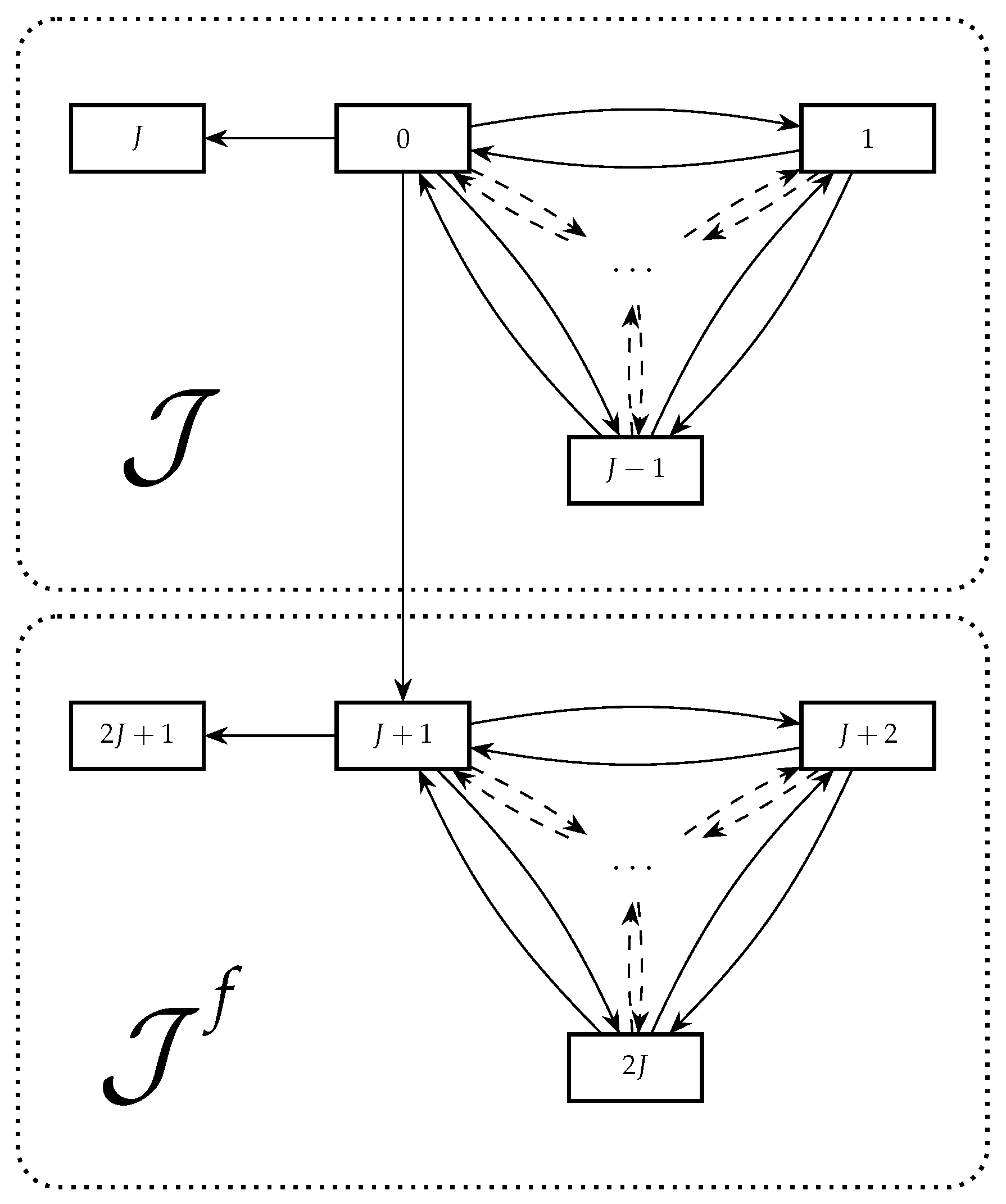
Policyholder behavior is modeled in the classic way by extending the state space of the Markov chain, Z, to include surrender and free policy states, as presented in Henriksen et al. (2014), and the state space of Z from Section 2 is extended, as illustrated in Figure 11. We do not consider the modeling or derivation of the surrender rate and the free-policy rate. The modeling of optimal surrender rates is studied in, for instance, De Giovanni (2010), Loisel and Milhaud (2011), and Barsotti et al. (2016), but little attention has been paid in existing literature to the choice of free-policy rate, which is often modeled as a deterministic intensity as in Henriksen et al. (2014) and Buchardt and Møller (2015). The extension of the state space in Figure 1 can also be obtained as a specific case of the more general state space expansion in Christiansen and Djehiche (2020).

The state J corresponds to surrender, and we assume that surrender can only happen from state 0. The state space ${\mathcal{J}}^f$ denotes the free-policy states, and it is a copy of $\mathcal{J}$ in the sense that it holds the same number of states and that state $i\in {\mathcal{J}}^f$ corresponds to state $i-(J+1)\in \mathcal{J}$. We assume that conversion to free-policy can only occur from state 0 and that the transition intensities in ${\mathcal{J}}^f$ equal the transition intensities in $\mathcal{J}$. We assume throughout the rest of this paper that $Z\left(0\right)\in \mathcal{J}$. The classical 7-state model from, for example, Buchardt and Møller (2015), is contained in this setup, where state 0 in our model corresponds to the premium-paying active state.

In order to model payments including policyholder behavior, the payment streams from Equation (1) are decomposed in benefits, $\mathrm{d}{B}_i^{+}\left(t\right)$, and premiums, $\mathrm{d}{B}_i^{-}\left(t\right)$, for $i=1,2$. The sojourn payments and payments upon transition are then decomposed in $b_i^{j+}$ and $b_i^{j-}$, and $b_i^{jk+}$ and $b_i^{jk-}$, respectively. We consider defined contributions such that the payment stream increased by bonus only contains benefits, i.e., $b_2^{j-}\left(t\right)=b_2^{jk-}\left(t\right)=0$ for all $t\ge 0$ and $j,k\in \mathcal{J}$, $j\ne k$.

The technical benefit and premium reserves, respectively, in the non-free-policy states, $Z\left(t\right)\in \mathcal{J}$, are given by

$$\begin{array}{c}\hfill V_i^{*Z\left(t\right)\pm }\left(t\right)={\mathbb{E}}^{*}\left[{\int }_t^n{e}^{-{\int }_t^s{r}^{*}\left(u\right)\mathrm{d}u}\mathrm{d}{B}_i^{\pm }\left(s\right)|Z\left(t\right)\right],\end{array}$$

for $i=1,2$, and where n is termination of the insurance contract.

Defined contributions imply that

$$\begin{array}{c}\hfill V_2^{*Z\left(t\right)}\left(t\right)=V_2^{*Z\left(t\right)+}\left(t\right)+V_2^{*Z\left(t\right)-}\left(t\right)=V_2^{*Z\left(t\right)+}\left(t\right),\end{array}$$

(5)

for $Z\left(t\right)\in \mathcal{J}$.

The duration U in the free-policy states is

$$\begin{array}{c}\hfill U\left(t\right)=inf\{s\in [0,t\left]\right|Z(t-s)\in \mathcal{J}\}.\end{array}$$

Payments in the free-policy states equal a free-policy factor, $f\in [0,1]$, times the benefits in the corresponding premium-paying state. We allow the free-policy factor to depend on the savings account, i.e., $f(t,X(t\left)\right)$, and the benefits are reduced with the free-policy factor evaluated at the time of conversion to free-policy, $f(t-U(t),X(t-U\left(t\right)\left)\right)$. We introduce the mapping of $Z\left(t\right)$ that returns the corresponding premium-paying state if $Z\left(t\right)\in {\mathcal{J}}^f$

$$\begin{array}{c}\hfill g\left(Z\left(t\right)\right)={𝟙}_{\{Z\left(t\right)\in {\mathcal{J}}^f\}}\left(Z\left(t\right)-(J+1)\right).\end{array}$$

Policyholder behavior is modeled solely on the market basis; therefore, ${\mu }_{0J}^{*}\left(t\right)={\mu }_{0(J+1)}^{*}\left(t\right)=0$ for all $t\ge 0$. The remaining transition intensities in ${\mathcal{J}}^f$ equal the corresponding transition intensities in $\mathcal{J}$ on the technical basis. Hence, the technical reserve in a free-policy state equals the free-policy factor times the technical benefit reserve in the corresponding premium-paying state

$$\begin{array}{c}\hfill V_i^{*Z\left(t\right)}\left(t\right)=f(t-U\left(t\right),X(t-U\left(t\right)))V_i^{*g\left(Z\right(t\left)\right)+}\left(t\right),\end{array}$$

for $i=1,2$ and $Z\left(t\right)\in {\mathcal{J}}^f$.

The inclusion of policyholder behavior changes the payment process from Equation (3) and the sum-at-risk from Proposition 1. Now, the payment process and the sum-at-risk depend on time, the savings account, and the duration in the free-policy states.

Proposition 3.

The total payment process guaranteed at time t including policyholder behavior is

$$\begin{array}{cc}\hfill \mathrm{d}B(t,X(t),& U\left(t\right),X(t-U(t\left)\right))\hfill \\ \hfill =& b^{Z\left(t\right)}(t,X\left(t\right),U\left(t\right),X(t-U\left(t\right)))\mathrm{d}t\hfill \\ \hfill & +\sum _{k:k\ne Z(t-)}{b}^{Z(t-)k}(t,X(t-),U\left(t\right),X((t-U\left(t\right))-))\mathrm{d}{N}^k\left(t\right),\hfill \end{array}$$

where the continuous payment function during sojourns in states and the payment function upon transition between states are

$$\begin{array}{cc}\hfill b^j(t,x,& u,x^f)\hfill \\ \hfill =& {𝟙}_{\{j\in \mathcal{J}\}}\left(b_1^j\left(t\right)+\frac{x-V_1^{*j}\left(t\right)}{V_2^{*j+}\left(t\right)}{b}_2^j\left(t\right)\right)\hfill \\ \hfill & +{𝟙}_{\{j\in {\mathcal{J}}^f\}}\left(f(t-u,x^f)b_1^{g\left(j\right)+}\left(t\right)+\frac{x-V_1^{*g\left(j\right)+}\left(t\right)f(t-u,x^f)}{V_2^{*g\left(j\right)+}\left(t\right)}{b}_2^{g\left(j\right)+}\left(t\right)\right),\hfill \\ \\ \hfill b^{jk}(t,x,& u,x^f)\hfill \\ \hfill =& {𝟙}_{\{j,k\in \mathcal{J},j\ne k\}}\left(b_1^{jk}\left(t\right)+\frac{x-V_1^{*j}\left(t\right)}{V_2^{*j+}\left(t\right)}{b}_2^{jk}\left(t\right)\right)\hfill \\ \hfill & +{𝟙}_{\{j,k\in {\mathcal{J}}^f,j\ne k\}}f(t-u,x^f)b_1^{g\left(j\right)g\left(k\right)+}\left(t\right)\hfill \\ \hfill & +{𝟙}_{\{j,k\in {\mathcal{J}}^f,j\ne k\}}\frac{x-V_1^{*g\left(j\right)+}\left(t\right)f(t-u,x^f)}{V_2^{*g\left(j\right)+}\left(t\right)}{b}_2^{g\left(j\right)g\left(k\right)+}\left(t\right),\hfill \end{array}$$

for $j,k\in \mathcal{J}\cup {\mathcal{J}}^f$, $j\ne k$. We assume that there are no continuous payments in the surrender states, and that there is no payment upon transition between $\mathcal{J}$ and ${\mathcal{J}}^f$.

Proposition 4.

Including policyholder behavior, the sum-at-risk from Proposition 1 is

$$\begin{array}{cc}\hfill R^{*jk}(t,x,& u,x^f)\hfill \\ \hfill =& b^{jk}(t,x,u,x^f)\hfill \\ \hfill & +{𝟙}_{\{j,k\in \mathcal{J},j\ne k\}}\left(V_1^{*k}\left(t\right)+\frac{x-V_1^{*j}\left(t\right)}{V_2^{*j+}\left(t\right)}{V}_2^{*k+}\left(t\right)-x\right)\hfill \\ \hfill & +{𝟙}_{\{j,k\in {\mathcal{J}}^f,j\ne k\}}{V}_1^{*g\left(k\right)+}\left(t\right)f(t-u,x^f)\hfill \\ \hfill & +{𝟙}_{\{j,k\in {\mathcal{J}}^f,j\ne k\}}\left(\frac{x-V_1^{*g\left(j\right)+}\left(t\right)f(t-u,x^f)}{V_2^{*g\left(j\right)+}\left(t\right)}{V}_2^{*g\left(k\right)+}\left(t\right)-x\right)\hfill \\ \hfill & +{𝟙}_{\{j=0,k=J+1\}}\left(V_1^{*g\left(k\right)+}\left(t\right)f(t,x)+\frac{x-V_1^{*j}\left(t\right)}{V_2^{*j+}\left(t\right)}{V}_2^{*g\left(k\right)+}\left(t\right)f(t,x)-x\right).\hfill \end{array}$$

The last line corresponds to the sum-at-risk upon conversion to free-policy, where $u=0$.

Remark 1.

In the last line of the sum-at-risk from Proposition 4, $g\left(k\right)=g(J+1)=0=j$, and by Equation (5), the sum-at-risk upon conversion to free-policy is

$$\begin{array}{c}\hfill \left(x-V_1^{*0-}\left(t\right)\right)f(t,x)-x.\end{array}$$

The dynamics of the savings account, X, and the surplus, Y, including policyholder behavior are equal to the dynamics in Propositions 1 and 2, where the payment process and the sum-at-risk are given by Propositions 3 and 4. Thus, the dynamics of the savings account are

$$\begin{array}{cc}\hfill \mathrm{d}X\left(t\right)=& r^{*}\left(t\right)X\left(t\right)\mathrm{d}t-\mathrm{d}B(t,X\left(t\right),U\left(t\right),X(t-U\left(t\right)))+{\delta }^{Z\left(t\right)}(t,X\left(t\right),Y\left(t\right))\mathrm{d}t\hfill \\ \hfill & +\sum _{k:k\ne Z(t-)}{R}^{*Z(t-)k}(t,X(t-),U(t-),X((t-U(t-))-))\hfill \\ \hfill & \times \left(\mathrm{d}{N}^k\left(t\right)-{\mu }_{Z(t-)k}^{*}\left(t\right)\mathrm{d}t\right),\hfill \end{array}$$

(6)

and the dynamics of the surplus are

$$\begin{array}{cc}\hfill \mathrm{d}Y\left(t\right)=& r\left(t\right)Y\left(t\right)\mathrm{d}t-{\delta }^{Z\left(t\right)}(t,X\left(t\right),Y\left(t\right))\mathrm{d}t+c^{Z\left(t\right)}(t,X\left(t\right),U\left(t\right),X(t-U\left(t\right)))\mathrm{d}t\hfill \\ \hfill & -\sum _{k:k\ne Z(t-)}{R}^{*Z(t-)k}(t,X(t-),U(t-),X((t-U(t-))-))\hfill \\ \hfill & \times \left(\mathrm{d}{N}^k\left(t\right)-{\mu }_{Z(t-)k}\left(t\right)\mathrm{d}t\right),\hfill \end{array}$$

(7)

where the surplus contribution is given by

$$\begin{array}{c}\hfill c^j(t,x,u,x^f)=(r\left(t\right)-r^{*}\left(t\right))x+\sum _{k:k\ne j}{R}^{*jk}(t,x,u,x^f)({\mu }_{jk}^{*}\left(t\right)-{\mu }_{jk}\left(t\right)).\end{array}$$

The dividend strategy $\delta$ is given by Equation (4).

The above dynamics of the savings account and the surplus contain the free-policy factor, f, and the duration, $U\left(t\right)$, which implies that they are not in the form of Lemma 1. Therefore, Theorem 1 cannot be used to project the savings account and the surplus including policyholder behavior.

5. State-Wise Projections Including Policyholder Behavior

In this section, the main results of the paper are presented by extending the result from Section 3 to include policyholder behavior. First, we describe the inclusion of policyholder behavior in the life insurance setup with bonus and the choice of free-policy factor. In general, the inclusion of the ideal choice of free-policy factor breaks the linearity assumption of Section 3. We consider a certain case where the linearity assumption is satisfied, and suggest an approximation of the ideal free-policy factor. The main results of this paper are that, in the certain case, the state-wise projections of the savings account and the surplus with the ideal free-policy factor and the approximated free-policy factor, respectively, coincide and that we extend Theorem 1 to include policyholder behavior in a general case.

5.1. Policyholder Behavior Including Bonus

The extension of the classic life insurance setup without bonus to include policyholder behavior is described in existing literature. See Buchardt et al. (2014) or Buchardt and Møller (2015) for a description of this extension. Without bonus, the payment upon surrender is usually chosen to be the technical reserve in state 0, $b^{0J}\left(t\right)=V^{*0}\left(t\right)$, such that the insured receive their savings account upon surrender, the sum-at-risk upon surrender is equal to zero, and the modeling of surrender can be omitted on the technical basis. Without bonus, the technical reserve, $V^{*}\left(t\right)$, is the technical value of future payments guaranteed at time t, since all payments are guaranteed. In our setup with bonus, this corresponds to the savings account, $X\left(t\right)$. The payment upon surrender in the setup with bonus is equal to the savings account $X\left(t\right)$ such that bonus obtained prior to time t is included in the payment upon surrender. Then, the sum-at-risk of the savings account upon surrender is equal to zero. This complies with the assumption that payments are linear in the savings account.

Without bonus, the free-policy factor is usually chosen according to the principle of equivalence such that there is no jump in the technical reserve upon conversion to free-policy, i.e.,

$$\begin{array}{c}\hfill f^{\circ }\left(t\right)=\frac{V^{*0}\left(t\right)}{V^{*0+}\left(t\right)},\end{array}$$

where the superscript ∘ refer to the setup without bonus.

To resemble the setup without bonus, the ideal free-policy factor in the setup with bonus is the free-policy factor, where the sum-at-risk of the savings account upon conversion to free-policy is equal to zero, resulting in no jump in X upon conversion to free-policy. The sum-at-risk upon conversion to free-policy is given in Remark 1, and setting this equal to zero implies that

$$\begin{array}{c}\hfill f(t,X(t-))=\frac{X(t-)}{X(t-)-V_1^{*0-}\left(t\right)}.\end{array}$$

(8)

This free-policy factor is nonlinear in the savings account, which implies that the dynamics of the savings account and the surplus from Equations (6) and (7) do not satisfy the linearity assumption in Lemma 1 with this choice of free-policy factor.

The objective when including policyholder behavior is to ensure that the savings account is unaffected when the behavior option is exercised. This is achieved when the sum-at-risk is equal to zero upon surrender and upon conversion to free-policy. In the study of prospective reserves, Christiansen and Djehiche (2020) denote this concept actuarial equivalence and obtain adjustment factors similar to our free-policy factor, but their adjustment factors depend on the prospective reserve, whereas our free-policy factor depends on the retrospective savings account.

Let $X_{\mathrm{id}}$ be the savings account and let $Y_{\mathrm{id}}$ be the surplus with the ideal free-policy factor from Equation (8) above. Similar to Definition 2, the state-wise projections of the savings account and the surplus are given by

$$\begin{array}{cc}\hfill & {\tilde{X}}_{\mathrm{id}}^j\left(t\right)={\mathbb{E}}_{Z\left(0\right)}\left[{𝟙}_{\left\{Z\right(t)=j\}}{X}_{\mathrm{id}}\left(t\right)|{\mathcal{F}}_t^r\right],\hfill \end{array}$$

(9)

$$\begin{array}{cc}\hfill & {\tilde{Y}}_{\mathrm{id}}^j\left(t\right)={\mathbb{E}}_{Z\left(0\right)}\left[{𝟙}_{\left\{Z\right(t)=j\}}{Y}_{\mathrm{id}}\left(t\right)|{\mathcal{F}}_t^r\right],\hfill \end{array}$$

(10)

for $j\in \mathcal{J}\cup {\mathcal{J}}^f$.

5.2. The Case with All Benefits Regulated by Bonus

We consider the case, where all benefits are regulated by bonus such that the payment stream not increased by bonus, $B_1$, only contains premiums, i.e., $B_1^{+}=0$. In this case, we show that the dynamics of the savings account and the surplus with the ideal free-policy factor from Equation (8), are in the form of Lemma 1 such that Theorem 1 can be used to find differential equations for the state-wise projections of the savings account and the surplus including policyholder behavior.

In the example of an insurance contract consisting of a life annuity and a term insurance, both products are regulated by bonus in the case $B_1^{+}=0$, in contrast to the case where only the life annuity is scaled by bonus.

The assumptions of defined contributions and $B_1^{+}=0$ imply that the total payment process has dynamics

$$\begin{array}{c}\hfill \mathrm{d}{B}_1^{-}\left(t\right)+Q(t-)\mathrm{d}{B}_2^{+}\left(t\right),\end{array}$$

where $Q(0-)=1$ due to the principle of equivalence.

In the continuous payment functions during sojourns in states and the payment functions upon transition between states from Proposition 3, the terms including the free-policy factor are multiplied by either $b_1^{j+}$, $b_1^{jk+}$ or $V_1^{*j+}$ for $j,k\in \mathcal{J}$. In the case $B_1^{+}=0$, these are all equal to zero; therefore, the free-policy factor does not appear in the payment functions.

The continuous payment functions during sojourns in states and the payment functions upon transition between states from Proposition 3 are, in this case,

$$\begin{array}{cc}\hfill b^j(t,x)=& {𝟙}_{\{j\in \mathcal{J}\}}\left(b_1^{j-}\left(t\right)+\frac{x-V_1^{*j-}\left(t\right)}{V_2^{*j+}\left(t\right)}{b}_2^{j+}\left(t\right)\right)\hfill \\ \hfill & +{𝟙}_{\{j\in {\mathcal{J}}^f\}}\left(\frac{x}{V_2^{*g\left(j\right)+}\left(t\right)}{b}_2^{g\left(j\right)+}\left(t\right)\right),\hfill \end{array}$$

(11)

$$\begin{array}{cc}\hfill b^{jk}(t,x)=& {𝟙}_{\{j,k\in \mathcal{J},j\ne k\}}\left(b_1^{jk-}\left(t\right)+\frac{x-V_1^{*j-}\left(t\right)}{V_2^{*j+}\left(t\right)}{b}_2^{jk+}\left(t\right)\right)\hfill \\ \hfill & +{𝟙}_{\{j,k\in {\mathcal{J}}^f,j\ne k\}}\left(\frac{x}{V_2^{*g\left(j\right)+}\left(t\right)}{b}_2^{g\left(j\right)g\left(k\right)+}\left(t\right)\right),\hfill \end{array}$$

(12)

for $j,k\in \mathcal{J}\cup {\mathcal{J}}^f$.

Similar to the payment functions, the terms including the free-policy factor in the sum-at-risk from Proposition 4 are multiplied by $V_1^{*j+}$ for $j\in \mathcal{J}$, except for the sum-at-risk upon conversion to free-policy. Thus, in the case $B_1^{+}=0$, the sum-at-risk is

$$\begin{array}{cc}\hfill R^{*jk}(t,x)=& b^{jk}(t,x)+{𝟙}_{\{j,k\in \mathcal{J},j\ne k\}}\left(V_1^{*k-}\left(t\right)+\frac{x-V_1^{*j-}\left(t\right)}{V_2^{*j+}\left(t\right)}{V}_2^{*k+}\left(t\right)-x\right)\hfill \\ \hfill & +{𝟙}_{\{j,k\in {\mathcal{J}}^f,j\ne k\}}\left(\frac{x}{V_2^{*g\left(j\right)+}\left(t\right)}{V}_2^{*g\left(k\right)+}\left(t\right)-x\right)\hfill \\ \hfill & +{𝟙}_{\{j=0,k=J+1\}}\left(\left(x-V_1^{*j-}\left(t\right)\right)f(t,x)-x\right).\hfill \end{array}$$

(13)

With the free-policy factor from Equation (8), the last line in the sum-at-risk above is equal to zero. Therefore, in the case $B_1^{+}=0$ with the free-policy factor from Equation (8), neither the payment functions (11) and (12) nor the sum-at-risk (13) depend on the duration in the free-policy states, and they are linear in the savings account. This implies that the dynamics of $X_{\mathrm{id}}\left(t\right)$ and $Y_{\mathrm{id}}\left(t\right)$ are in the form of Lemma 1, leading to the result in Theorem 1. Hence, in this case, we actually have differential equations for the projected savings account and the projected surplus with the free-policy factor from Equation (8) given by

$$\begin{array}{cc}\hfill \frac{\mathrm{d}}{\mathrm{d}t}{\tilde{X}}_{\mathrm{id}}^j\left(t\right)=& \sum _{k:k\ne j}{\mu }_{kj}\left(t\right){\tilde{X}}_{\mathrm{id}}^k\left(t\right)-\sum _{k:k\ne j}{\mu }_{jk}\left(t\right){\tilde{X}}_{\mathrm{id}}^j\left(t\right)+{\widehat{\alpha }}_{0,X}^j\left(t\right)p_{Z\left(0\right)j}(0,t)+{\widehat{\alpha }}_{1,X}^j\left(t\right){\tilde{X}}_{\mathrm{id}}^j\left(t\right)\hfill \\ \hfill & +{\widehat{\alpha }}_{2,X}^j\left(t\right){\tilde{Y}}_{\mathrm{id}}^j\left(t\right)+\sum _{k:k\ne j}{\mu }_{kj}\left(t\right)\left({\widehat{\lambda }}_{0,X}^{kj}\left(t\right)p_{Z\left(0\right)k}(0,t)+{\widehat{\lambda }}_{1,X}^{kj}\left(t\right){\tilde{X}}_{\mathrm{id}}^k\left(t\right)\right),\hfill \end{array}$$

(14)

$$\begin{array}{cc}\hfill \frac{\mathrm{d}}{\mathrm{d}t}{\tilde{Y}}_{\mathrm{id}}^j\left(t\right)=& \sum _{k:k\ne j}{\mu }_{kj}\left(t\right){\tilde{Y}}_{\mathrm{id}}^k\left(t\right)-\sum _{k:k\ne j}{\mu }_{jk}\left(t\right){\tilde{Y}}_{\mathrm{id}}^j\left(t\right)+{\widehat{\alpha }}_{0,Y}^j\left(t\right)p_{Z\left(0\right)j}(0,t)+{\widehat{\alpha }}_{1,Y}^j\left(t\right){\tilde{X}}_{\mathrm{id}}^j\left(t\right)\hfill \\ \hfill & +{\widehat{\alpha }}_{2,Y}^j\left(t\right){\tilde{Y}}_{\mathrm{id}}^j\left(t\right)+\sum _{k:k\ne j}{\mu }_{kj}\left(t\right)\left({\widehat{\lambda }}_{0,Y}^{kj}\left(t\right)p_{Z\left(0\right)k}(0,t)+{\widehat{\lambda }}_{1,Y}^{kj}\left(t\right){\tilde{X}}_{\mathrm{id}}^k\left(t\right)\right),\hfill \end{array}$$

(15)

and ${\tilde{X}}_{i\mathrm{d}}^j(0-)={\tilde{Y}}_{i\mathrm{d}}^j(0-)=0$ for $j\in \mathcal{J}\cup {\mathcal{J}}^f$. The expressions for ${\widehat{\alpha }}^j$ and ${\widehat{\lambda }}^{jk}$ are in Appendix B.

We compare the differential equations of the projected savings account and the projected surplus in the case $B_1^{+}=0$ using the free-policy factor from Equation (8) with the differential equations without policyholder behavior. This comes down to a comparison of the coefficients ${\alpha }^j$ and ${\lambda }^{jk}$ from Appendix A and ${\widehat{\alpha }}^j$ and ${\widehat{\lambda }}^{jk}$ from Appendix B. The coefficient ${\alpha }^j$ and the corresponding ${\widehat{\alpha }}^j$ consist of the same terms, but ${\widehat{\alpha }}^j$ is decomposed in the cases $j\in \mathcal{J}$ and $j\in {\mathcal{J}}^f$ in the same sense as the payment functions and the sum-at-risk from Equations (11)–(13), since there are only benefits in the free-policy states. This also goes for ${\lambda }^{jk}$ and ${\widehat{\lambda }}^{jk}$.

Remark 2.

The case $B_1^{+}=B_2^{+}$ corresponds to the case $B_1^{+}=0$, since the total payment process when $B_1^{+}=B_2^{+}$ is

$$\begin{array}{c}\hfill \mathrm{d}{B}_1\left(t\right)+Q(t-)\mathrm{d}{B}_2^{+}\left(t\right)=\mathrm{d}{B}_1^{-}\left(t\right)+(\underset{=\tilde{Q}(t-)}{\underbrace{1+Q(t-)}})d{B}_2^{+}\left(t\right),\end{array}$$

which has the same form as the payment process in the case $B_1^{+}=0$, but where $\tilde{Q}(0-)=2$ since $Q(0-)=1$ due to the principle of equivalence. When the benefits in $B_1$ are equal to the benefits in $B_2$, all benefits are regulated equally by bonus; therefore, the case $B_1^{+}=B_2^{+}$ can be rewritten to be in the form of $B_1^{+}=0$. Hence, the results above also apply for $B_1^{+}=B_2^{+}$.

If benefits not regulated by bonus cancel due to conversion to free-policy, $B_1^{+}=0$ after conversion to free-policy, and the result above still applies. An example is an insurance contract consisting of a life annuity and a term insurance, where the life annuity is regulated by bonus, and the term insurance cancels upon conversion to free-policy. Throughout this paper, we assume that payments in the free-policy states equal a free-policy factor times the benefits in the corresponding premium-paying state. The example does not comply with this assumption, but we can easily extend our setup to include this case.

5.3. Approximation of the Free-Policy Factor

In the general setup, $B_1^{+}\left(t\right)\ge 0$ for $t\ge 0$, we cannot project the savings account and the surplus including policyholder behavior by Theorem 1, since the assumptions are violated. The dynamics of the savings account and the surplus depend on the duration in the free-policy states, U. Furthermore, the derivation of Theorem 1 relies on linearity of X and Y in the dynamics from Lemma 1, which breaks when the free-policy factor depends on the savings account. This motivates an approximation of the ideal free-policy factor from Equation (8), which does not depend on X.

Just before conversion to free-policy, the policyholder must be premium paying and active, i.e., $Z(t-)=0$. A reasonable approximation of the free-policy factor is, therefore,

$$\begin{array}{c}\hfill \widehat{f}\left(t\right)={\mathbb{E}}_{Z\left(0\right)}\left[{𝟙}_{\left\{Z\right(t-)=0\}}f(t,X\left(t\right))|{\mathcal{F}}_t^r\right]={\mathbb{E}}_{Z\left(0\right)}\left[{𝟙}_{\left\{Z\right(t-)=0\}}\frac{X(t-)}{X(t-)-V_1^{*Z(t-)-}\left(t\right)}|{\mathcal{F}}_t^r\right].\end{array}$$

We have not developed methods to calculate the projection of a fraction containing the savings account, $X\left(t\right)$, in both the nominator and the denominator. Therefore, we cannot continue with the approximation above. Alternatively, the nominator and denominator in the free-policy factor can be projected separately:

$$\begin{array}{cc}\hfill \tilde{f}\left(t\right)& =\frac{{\mathbb{E}}_{Z\left(0\right)}\left[{𝟙}_{\left\{Z\right(t-)=0\}}X(t-)|{\mathcal{F}}_t^r\right]}{{\mathbb{E}}_{Z\left(0\right)}\left[{𝟙}_{\left\{Z\right(t-)=0\}}\left(X(t-)-V_1^{*Z(t-)-}\left(t\right)\right)|{\mathcal{F}}_t^r\right]}\hfill \\ \hfill & =\frac{{\tilde{X}}^0\left(t\right)}{{\tilde{X}}^0\left(t\right)-p_{Z\left(0\right)0}(0,t)V_1^{*0-}\left(t\right)}.\hfill \end{array}$$

(16)

The above free-policy factor does not depend on the savings account, but on the state-wise projection of the savings account. This approximation of the ideal free-policy factor motivates one of the main results of this paper presented in Corollary 1 below.

Corollary 1.

Let $X_{id}$ be the savings account and $Y_{id}$ be the surplus modeled with the ideal free-policy factor from Equation (8), and let $X_{ap}$ be the savings account and $Y_{ap}$ be the surplus modeled with the approximated free-policy factor from Equation (16). The state-wise projections are given by Equations (9) and (10), and

$$\begin{array}{cc}\hfill & {\tilde{X}}_{ap}^j\left(t\right)={\mathbb{E}}_{Z\left(0\right)}\left[{𝟙}_{\left\{Z\right(t)=j\}}{X}_{ap}\left(t\right)|{\mathcal{F}}_t^r\right],\hfill \\ \hfill & {\tilde{Y}}_{ap}^j\left(t\right)={\mathbb{E}}_{Z\left(0\right)}\left[{𝟙}_{\left\{Z\right(t)=j\}}{Y}_{ap}\left(t\right)|{\mathcal{F}}_t^r\right],\hfill \end{array}$$

for $j\in \mathcal{J}\cup {\mathcal{J}}^f$, respectively.

In the case where all benefits are regulated by bonus, $B_1^{+}=0$

$$\begin{array}{cc}\hfill & {\tilde{X}}_{id}^j\left(t\right)={\tilde{X}}_{ap}^j\left(t\right),\hfill \\ \hfill & {\tilde{Y}}_{id}^j\left(t\right)={\tilde{Y}}_{ap}^j\left(t\right),\hfill \end{array}$$

for $j\in \mathcal{J}\cup {\mathcal{J}}^f$.

Proof. 

Assume all benefits are regulated by bonus, $B_1^{+}=0$. The state-wise projections of the savings account and the surplus with the ideal free-policy factor satisfy the differential equations in Equations (14) and (15).

Equations (11)–(13) in Section 5.2 state that only the sum-at-risk depends on the free-policy factor. The sum-at-risk with the approximated free-policy factor, $\tilde{f}$, is

$$\begin{array}{cc}\hfill R^{*jk}(t,x)=& b^{jk}(t,x)+{𝟙}_{\{j,k\in \mathcal{J},j\ne k\}}\left(V_1^{*k-}\left(t\right)+\frac{x-V_1^{*j-}\left(t\right)}{V_2^{*j+}\left(t\right)}{V}_2^{*k+}\left(t\right)-x\right)\hfill \\ \hfill & +{𝟙}_{\{j,k\in {\mathcal{J}}^f,j\ne k\}}\left(\frac{x}{V_2^{*g\left(j\right)+}\left(t\right)}{V}_2^{*g\left(k\right)+}\left(t\right)-x\right)\hfill \\ \hfill & +{𝟙}_{\{j=0,k=J+1\}}\left(\left(x-V_1^{*j-}\left(t\right)\right)\tilde{f}\left(t\right)-x\right).\hfill \end{array}$$

(17)

The dynamics of $X_{\mathrm{ap}}$ and $Y_{\mathrm{ap}}$ are in the form of Equations (6) and (7) with the payment functions from Equations (11) and (12) and the sum-at-risk from Equation (17). This implies that the dynamics of $X_{\mathrm{ap}}$ and $Y_{\mathrm{ap}}$ are in the same form as in Lemma 1, since they do not depend on the duration, U, and they are linear in $X_{\mathrm{ap}}\left(t\right)$ and $Y_{\mathrm{ap}}\left(t\right)$.

Theorem 1 gives differential equations of the state-wise projections of the savings account and the surplus, ${\tilde{X}}_{\mathrm{ap}}^j$ and ${\tilde{Y}}_{\mathrm{ap}}^j$. These differential equations can be expressed in terms of $\widehat{\alpha }$ and $\widehat{\lambda }$ from the differential Equations (14) and (15)

$$\begin{array}{cc}\hfill \frac{\mathrm{d}}{\mathrm{d}t}{\tilde{X}}_{\mathrm{ap}}^j\left(t\right)=& \sum _{k:k\ne j}{\mu }_{kj}\left(t\right){\tilde{X}}_{\mathrm{ap}}^k\left(t\right)-\sum _{k:k\ne j}{\mu }_{jk}\left(t\right){\tilde{X}}_{\mathrm{ap}}^j\left(t\right)+{\widehat{\alpha }}_{0,X}^j\left(t\right)p_{Z\left(0\right)j}(0,t)+{\widehat{\alpha }}_{1,X}^j\left(t\right){\tilde{X}}_{\mathrm{ap}}^j\left(t\right)\hfill \\ \hfill & +{\widehat{\alpha }}_{2,X}^j\left(t\right){\tilde{Y}}_{\mathrm{ap}}^j\left(t\right)+{𝟙}_{\{j=J+1\}}{\mu }_{0j}^{*}\left(t\right)\left({\tilde{X}}_{\mathrm{ap}}^0\left(t\right)+\tilde{f}\left(t\right)\left(p_{Z\left(0\right)0}(0,t)V_1^{*0-}\left(t\right)-{\tilde{X}}_{\mathrm{ap}}^0\left(t\right)\right)\right)\hfill \\ \hfill & +\sum _{k:k\ne j}{\mu }_{kj}\left(t\right)({\widehat{\lambda }}_{0,X}^{kj}\left(t\right)p_{Z\left(0\right)k}(0,t)+{\widehat{\lambda }}_{1,X}^{kj}\left(t\right){\tilde{X}}_{\mathrm{ap}}^k\left(t\right)r\hfill \\ \hfill & -{𝟙}_{\{k=0,j=J+1\}}({\tilde{X}}_{\mathrm{ap}}^0\left(t\right)+\tilde{f}\left(t\right)(p_{Z\left(0\right)0}(0,t)V_1^{*0-}\left(t\right)-{\tilde{X}}_{\mathrm{ap}}^0(t)\left)\right)),\hfill \end{array}$$

(18)

$$\begin{array}{cc}\hfill \frac{\mathrm{d}}{\mathrm{d}t}{\tilde{Y}}_{\mathrm{ap}}^j\left(t\right)=& \sum _{k:k\ne j}{\mu }_{kj}\left(t\right){\tilde{Y}}_{\mathrm{ap}}^k\left(t\right)-\sum _{k:k\ne j}{\mu }_{jk}\left(t\right){\tilde{Y}}_{\mathrm{ap}}^j\left(t\right)+{\widehat{\alpha }}_{0,Y}^j\left(t\right)p_{Z\left(0\right)j}(0,t)+{\widehat{\alpha }}_{1,Y}^j\left(t\right){\tilde{X}}_{\mathrm{ap}}^j\left(t\right)\hfill \\ \hfill & +{\widehat{\alpha }}_{2,Y}^j\left(t\right){\tilde{Y}}_{\mathrm{ap}}^j\left(t\right)-{𝟙}_{\{j=J+1\}}{\mu }_{0j}^{*}\left(t\right)\left({\tilde{X}}_{\mathrm{ap}}^0\left(t\right)+\tilde{f}\left(t\right)\left(p_{Z\left(0\right)0}(0,t)V_1^{*0-}\left(t\right)-{\tilde{X}}_{\mathrm{ap}}^0\left(t\right)\right)\right)\hfill \\ \hfill & +\sum _{k:k\ne j}{\mu }_{kj}\left(t\right)({\widehat{\lambda }}_{0,Y}^{kj}\left(t\right)p_{Z\left(0\right)k}(0,t)+{\widehat{\lambda }}_{1,Y}^{kj}\left(t\right){\tilde{X}}_{\mathrm{ap}}^k\left(t\right)\hfill \\ \hfill & +{𝟙}_{\{k=0,j=J+1\}}\left({\tilde{X}}_{\mathrm{ap}}^0\left(t\right)+\tilde{f}\left(t\right)\left(p_{Z\left(0\right)0}(0,t)V_1^{*0-}\left(t\right)-{\tilde{X}}_{\mathrm{ap}}^0\left(t\right)\right)\right)).\hfill \end{array}$$

(19)

By inserting the expression for $\tilde{f}$ from Equation (16), the differential Equations (18) and (19) are equal to the differential Equations (14) and (15). Furthermore, the initial conditions are

$$\begin{array}{c}\hfill {\tilde{X}}_{\mathrm{id}}^j\left(0\right)={\tilde{Y}}_{\mathrm{id}}^j\left(0\right)={\tilde{X}}_{\mathrm{ap}}^j\left(0\right)={\tilde{Y}}_{\mathrm{ap}}^j\left(0\right)=0,\end{array}$$

for $j\in \mathcal{J}\cup {\mathcal{J}}^f$. This implies that

$$\begin{array}{cc}\hfill & {\tilde{X}}_{\mathrm{id}}^j\left(t\right)={\tilde{X}}_{\mathrm{ap}}^j\left(t\right),\hfill \\ \hfill & {\tilde{Y}}_{\mathrm{id}}^j\left(t\right)={\tilde{Y}}_{\mathrm{ap}}^j\left(t\right),\hfill \end{array}$$

for $j\in \mathcal{J}\cup {\mathcal{J}}^f$, as desired. □

Corollary 1 implies that, in the case $B_1^{+}=0$, we can project the savings account and the surplus with the approximated free-policy factor and actually obtain the same accurate projections as with the ideal free-policy factor. Based on this result, we consider $\tilde{f}$ to be a reasonable approximation of f, which does not depend on the savings account but, instead, on the projected savings account.

5.4. Projections with the Approximated Free-Policy Factor

In the general setup, $B_1^{+}\left(t\right)\ge 0$ for $t\ge 0$, with the approximated free-policy factor from Equation (16), the dynamics of the savings account and the surplus are linear, but they also depend on the duration through the payment functions from Proposition 3 and the sum-of-risk from Proposition 4. Therefore, we cannot use Theorem 1 to project the savings account and the surplus. This motivates an extension of Theorem 1 including duration dependence, where linearity in the dynamics of the savings account and the surplus is preserved.

Lemma 2.

The dynamics of the savings account, $X_{ap}$, from Equation (6) and the dynamics of the surplus, $Y_{ap}$, from Equation (7), with the approximated free-policy factor, $\tilde{f}$, from Equation (16), can be written in the form

$$\begin{array}{cc}\hfill \mathrm{d}{X}_{ap}\left(t\right)=& \left({\overline{\alpha }}_{0,X}^{Z\left(t\right)}\left(t\right)+{\overline{\alpha }}_{1,X}^{Z\left(t\right)}\left(t\right)X_{ap}\left(t\right)+{\overline{\alpha }}_{2,X}^{Z\left(t\right)}\left(t\right)Y_{ap}\left(t\right)+\tilde{f}(t-U\left(t\right)){\overline{\beta }}_{0,X}^{Z\left(t\right)}\left(t\right)\right)\mathrm{d}t\hfill \\ \hfill & +\sum _{k:k\ne Z(t-)}\left({\overline{\lambda }}_{0,X}^{Z(t-)k}\left(t\right)+{\overline{\lambda }}_{1,X}^{Z(t-)k}\left(t\right)X_{ap}(t-)+\tilde{f}(t-U\left(t\right)){\overline{\gamma }}_{0,X}^{Z(t-)k}\left(t\right)\right)\mathrm{d}{N}^k\left(t\right),\hfill \\ \hfill \mathrm{d}{Y}_{ap}\left(t\right)=& \left({\overline{\alpha }}_{0,Y}^{Z\left(t\right)}\left(t\right)+{\overline{\alpha }}_{1,Y}^{Z\left(t\right)}\left(t\right)X_{ap}\left(t\right)+{\overline{\alpha }}_{2,Y}^{Z\left(t\right)}\left(t\right)Y_{ap}\left(t\right)+\tilde{f}(t-U\left(t\right)){\overline{\beta }}_{0,Y}^{Z\left(t\right)}\left(t\right)\right)\mathrm{d}t\hfill \\ \hfill & +\sum _{k:k\ne Z(t-)}\left({\overline{\lambda }}_{0,Y}^{Z(t-)k}\left(t\right)+{\overline{\lambda }}_{1,Y}^{Z(t-)k}\left(t\right)X_{ap}(t-)+\tilde{f}(t-U\left(t\right)){\overline{\gamma }}_{0,Y}^{Z(t-)k}\left(t\right)\right)\mathrm{d}{N}^k\left(t\right),\hfill \end{array}$$

for deterministic functions ${\overline{\alpha }}_{i,H}^j,{\overline{\beta }}_{i,H}^j,{\overline{\lambda }}_{i,H}^{jk},{\overline{\gamma }}_{i,H}^{jk}$ for $i=0,1,2$, $H=X,Y$ and $j,k\in \mathcal{J}\cup {\mathcal{J}}^f$, $j\ne k$, where

$$\begin{array}{c}\hfill {\overline{\beta }}_{0,X}^j\left(t\right)={\overline{\beta }}_{0,Y}^j\left(t\right)={\overline{\gamma }}_{0,X}^{jk}\left(t\right)={\overline{\gamma }}_{0,Y}^{jk}\left(t\right)=0,\end{array}$$

for all $t\ge 0$ and $j\in \mathcal{J}$.

See Appendix C for the expressions of $\overline{\alpha },\overline{\beta },\overline{\lambda }$, and $\overline{\gamma }$ for the savings account and the surplus.

We consider the difference between the case with all benefits regulated by bonus, $B_1^{+}=0$, with the free-policy factor from Equation (8) from Section 5.2 and the general case, $B_1^{+}\ge 0$, with the approximated free-policy factor. This comes down to a comparison of the coefficients $\widehat{\alpha }$ and $\widehat{\lambda }$ from Appendix B with the coefficients $\overline{\alpha }$, $\overline{\beta }$, $\overline{\lambda }$, and $\overline{\gamma }$ from Appendix C. Apart from the sum-at-risk upon conversion to free-policy and the duration dependent terms, the coefficients are equal. In the first case, the sum-at-risk upon conversion to free-policy is equal to zero, while, in the second case, it is added to $\overline{\lambda }$. The duration dependent terms from Propositions 3 and 4 are equal to zero in the case with all benefits regulated by bonus, while, in the general case, they appear in $\overline{\beta }$ and $\overline{\gamma }$.

The dynamics of the savings account and the surplus in Lemma 2 allow for an extension of the dividend strategy from Equation (4) to be duration dependent. Dividends in form

$$\begin{array}{cc}\hfill & {\delta }^j(t,x,y,u)={\delta }_0^j(t,u)+{\delta }_1^j\left(t\right)·x+{\delta }_2^j\left(t\right)·y,\hfill \\ \hfill & {\delta }_0^j(t,u)={𝟙}_{\{j\in \mathcal{J}\}}{\delta }_0^j\left(t\right)+{𝟙}_{\{j\in {\mathcal{J}}^f\}}\tilde{f}(t-u){\delta }_0^j\left(t\right)\hfill \end{array}$$

comply with the dynamics in Lemma 2.

Now, we extend the result of Theorem 1 to include duration dependence in the approximated free-policy factor from the dynamics of the savings account and the surplus in Lemma 2.

Theorem 2.

Let $X_{\mathrm{ap}}$ and $Y_{\mathrm{ap}}$ have dynamics in the form of Lemma 2 and $Z\left(0\right)\in \mathcal{J}$. The state-wise projections of the savings account and the surplus, ${\tilde{X}}_{ap}^j$ and ${\tilde{Y}}_{ap}^j$, satisfy the system of differential equations below

$$\begin{array}{cc}\hfill \frac{\mathrm{d}}{\mathrm{d}t}{\tilde{X}}_{ap}^j\left(t\right)=& \sum _{k:k\ne j}{\mu }_{kj}\left(t\right){\tilde{X}}_{ap}^k\left(t\right)-\sum _{k:k\ne j}{\mu }_{jk}\left(t\right){\tilde{X}}_{ap}^j\left(t\right)+{\overline{\alpha }}_{0,X}^j\left(t\right)p_{Z\left(0\right)j}^{\tilde{f}}(0,t)+{\overline{\alpha }}_{1,X}^j\left(t\right){\tilde{X}}_{ap}^j\left(t\right)\hfill \\ \hfill & +{\overline{\alpha }}_{2,X}^j\left(t\right){\tilde{Y}}_{ap}^j\left(t\right)+\sum _{k:k\ne j}{\mu }_{kj}\left(t\right)\left({\overline{\lambda }}_{0,X}^{kj}\left(t\right)p_{Z\left(0\right)k}^{\tilde{f}}(0,t)+{\overline{\lambda }}_{1,X}^{kj}\left(t\right){\tilde{X}}_{ap}^k\left(t\right)\right)\hfill \\ \hfill & +{\overline{\beta }}_{0,X}^j\left(t\right)p_{Z\left(0\right)j}^{\tilde{f}}(0,t)+\sum _{k:k\ne j}{\mu }_{kj}\left(t\right){\overline{\gamma }}_{0,X}^{kj}\left(t\right)p_{Z\left(0\right)k}^{\tilde{f}}(0,t),\hfill \end{array}$$

$$\begin{array}{cc}\hfill \frac{\mathrm{d}}{\mathrm{d}t}{\tilde{Y}}_{ap}^j\left(t\right)=& \sum _{k:k\ne j}{\mu }_{kj}\left(t\right){\tilde{Y}}_{ap}^k\left(t\right)-\sum _{k:k\ne j}{\mu }_{jk}\left(t\right){\tilde{Y}}_{ap}^j\left(t\right)+{\overline{\alpha }}_{0,Y}^j\left(t\right)p_{Z\left(0\right)j}^{\tilde{f}}(0,t)+{\overline{\alpha }}_{1,Y}^j\left(t\right){\tilde{X}}_{ap}^j\left(t\right)\hfill \\ \hfill & +{\overline{\alpha }}_{2,Y}^j\left(t\right){\tilde{Y}}_{ap}^j\left(t\right)+\sum _{k:k\ne j}{\mu }_{kj}\left(t\right)\left({\overline{\lambda }}_{0,Y}^{kj}\left(t\right)p_{Z\left(0\right)k}^{\tilde{f}}(0,t)+{\overline{\lambda }}_{1,Y}^{kj}\left(t\right){\tilde{X}}_{ap}^k\left(t\right)\right)\hfill \\ \hfill & +{\overline{\beta }}_{0,Y}^j\left(t\right)p_{Z\left(0\right)j}^{\tilde{f}}(0,t)+\sum _{k:k\ne j}{\mu }_{kj}\left(t\right){\overline{\gamma }}_{0,Y}^{kj}\left(t\right)p_{Z\left(0\right)k}^{\tilde{f}}(0,t),\hfill \end{array}$$

where ${\tilde{X}}_{ap}^j(0-)={\tilde{Y}}_{ap}^j(0-)=0$, $\tilde{f}$ is the approximated free-policy factor from Equation (16), and $p_{Z\left(0\right)j}^{\tilde{f}}(0,t)$ are the $\tilde{f}$-modified probabilities

$$\begin{array}{c}\hfill p_{Z\left(0\right)j}^{\tilde{f}}(0,t)={\mathbb{E}}_{Z\left(0\right)}\left[{𝟙}_{\left\{Z\right(t)=j\}}\tilde{f}{(t-U\left(t\right))}^{{𝟙}_{\{j\in {\mathcal{J}}^f\}}}\right],\end{array}$$

for $Z\left(0\right)\in \mathcal{J}$, $j\in \mathcal{J}\cup {\mathcal{J}}^f$, and $t\ge 0$.

Proof. 

See Appendix D. □

Buchardt and Møller (2015) derive forward differential equations for the same $\tilde{f}$-modified probabilities in the case where $j\in {\mathcal{J}}^f$. In the case where $j\in \mathcal{J}$, the $\tilde{f}$-modified probabilities are the ordinary transition probabilities that satisfy Kolmogorov’s forward differential equations. Therefore, for a general $j\in \mathcal{J}\cup {\mathcal{J}}^f$, the $\tilde{f}$-modified probabilities satisfy the following forward differential equations

$$\begin{array}{cc}\hfill \frac{\mathrm{d}}{\mathrm{d}t}{p}_{Z\left(0\right)j}^{\tilde{f}}(0,t)=& {𝟙}_{\{j=J+1\}}{p}_{Z\left(0\right)0}^{\tilde{f}}(0,t){\mu }_{0(J+1)}\left(t\right)\tilde{f}\left(t\right)-p_{Z\left(0\right)j}^{\tilde{f}}(0,t)\sum _{k:k\ne j}{\mu }_{jk}\left(t\right)\hfill \\ \hfill & +{𝟙}_{\{j\in {\mathcal{J}}^f\}}\sum _{\begin{array}{c}k\in {\mathcal{J}}^f\\ k\ne j\end{array}}{p}_{Z\left(0\right)k}^{\tilde{f}}(0,t){\mu }_{kj}\left(t\right)+{𝟙}_{\{j\in \mathcal{J}\}}\sum _{\begin{array}{c}k\in \mathcal{J}\\ k\ne j\end{array}}{p}_{Z\left(0\right)k}^{\tilde{f}}(0,t){\mu }_{kj}\left(t\right).\hfill \end{array}$$

We consider Theorem 2 as one of the main results of the paper, since it enables us to project the savings account and the surplus in a general setup with the policyholder behavior options surrender and free-policy with the approximated free-policy factor from Equation (16), for instance, in the example with an insurance contract consisting of a life annuity and a term insurance, where the life annuity is regulated by bonus and the term insurance and the premiums are fixed.

Remark 3.

Let the savings account and the surplus have dynamics in the form of Lemma 2, but with a general free-policy factor, $\overline{f}$, that does not depend on the savings account. Then, Theorem 2 holds with $\overline{f}$-modified probabilities.

In the Danish life insurance business, it is common to scale all benefits (both those regulated by bonus and those not regulated by bonus) with the free-policy factor upon conversion to free-policy. We can imagine an insurance contract where only the benefits not regulated by bonus, $B_1^{+}$, are scaled with the free-policy factor upon conversion to free-policy and where $Q(0-)=0$. Then, the free-policy factor does not depend on the savings account, and Theorem 2 applies.

6. Numerical Simulation Example

In this section, we emphasize the practical applications of our results in a numerical simulation example and study the state-wise projections of the savings account and the surplus in a survival model including free-policy.

To illustrate this example, we assume the interest rate follow a Vasicek model with dynamics

$$\begin{array}{c}\hfill \mathrm{d}r\left(t\right)=(\varphi +\psi r\left(t\right))\mathrm{d}t+\sqrt{\theta }\mathrm{d}W\left(t\right),\end{array}$$

where ${\left(W\left(t\right)\right)}_{\{t\ge 0\}}$ is a Brownian motion; see, for instance, Björk (2009). Any other model of the interest rate can be chosen.

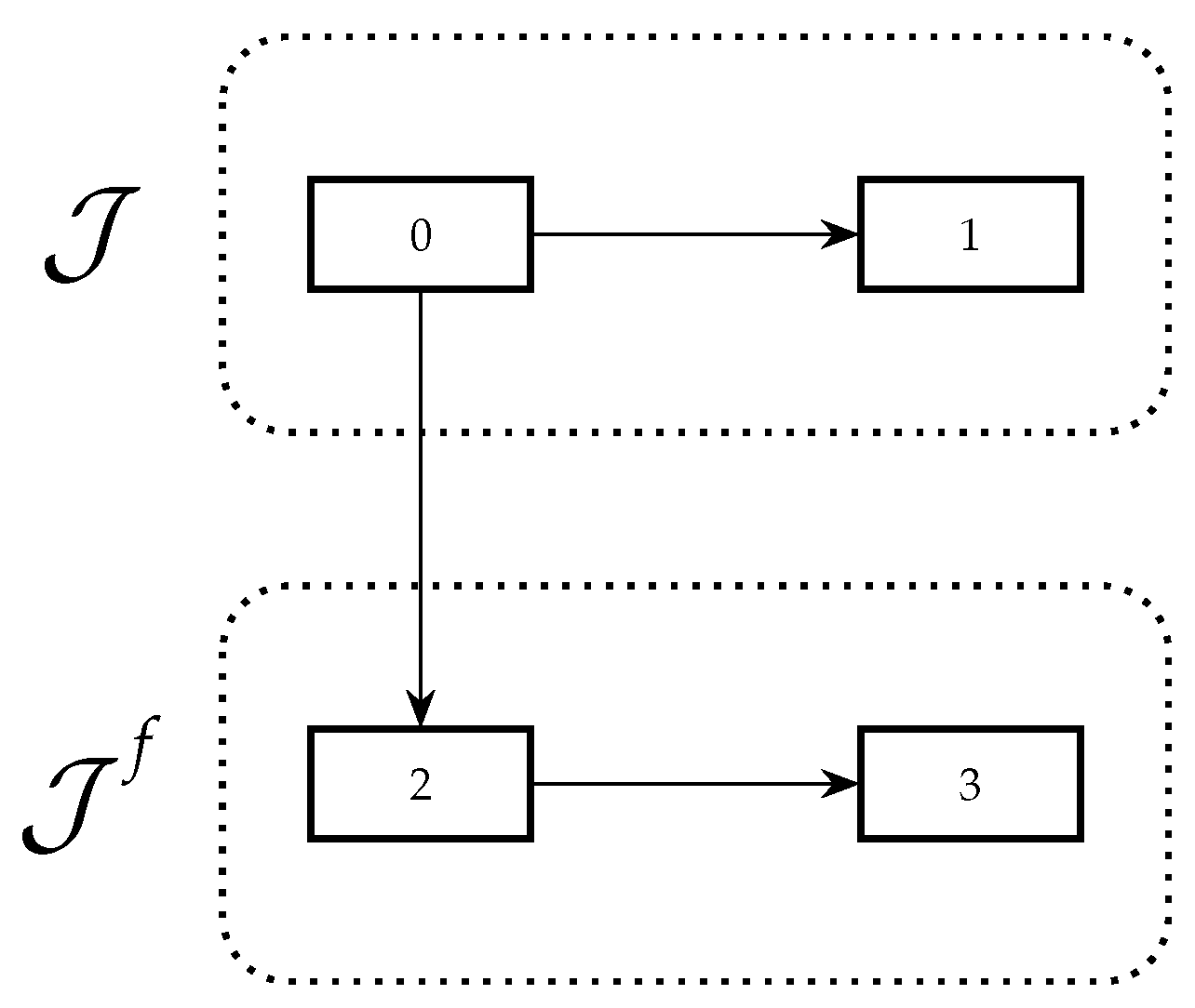
The survival model including free-policy is illustrated in Figure 22, where state 0 corresponds to alive, and state 1 corresponds to dead, in the non-free-policy states, and state 2 and state 3 corresponds to alive and dead, respectively, in the free-policy states. We consider an insured male at age $a_0$ at initialization of the insurance contract at time 0. The insurance contract consists of premiums paid continuously in state 0 until retirement age n, a term insurance not regulated by bonus payable upon dead before retirement age, and a life annuity regulated by bonus paid continuously when alive after retirement age. Hence, in this example, $B_1^{+}\ge 0$, and we use Theorem 2 in the projection. The payment process is

$$\begin{array}{cc}\hfill \mathrm{d}B(t,X(t\left)\right)=& {𝟙}_{\left\{Z\right(t)=0\}}\left(\left(\frac{X\left(t\right)-V_1^{*0}\left(t\right)}{V_2^{*0}\left(t\right)}{b}_2^0\left(t\right)-\pi \left(t\right)\right)\mathrm{d}t+b_1^{01}\left(t\right)\mathrm{d}{N}^1\left(t\right)\right)\hfill \\ \hfill & +{𝟙}_{\left\{Z\right(t)=2\}}\left(\frac{X\left(t\right)-\tilde{f}(t-U\left(t\right))V_1^{*0}\left(t\right)}{V_2^{*0}\left(t\right)}{b}_2^0\left(t\right)\mathrm{d}t+\tilde{f}(t-U\left(t\right))b_1^{01}\left(t\right)\mathrm{d}{N}^3\left(t\right)\right).\hfill \end{array}$$

The premium rate is determined according to the principle of equivalence on the technical basis, and we use the approximated free-policy factor from Equation (16).

Inspired by Bruhn and Lollike (2020), we choose a dividend strategy equal to

$$\begin{array}{cc}\hfill {\delta }^{Z\left(t\right)}(t,U\left(t\right),X\left(t\right),Y\left(t\right))=& 0.5·{\left(r\left(t\right)-r^{*}\left(t\right)\right)}^{+}X\left(t\right)+0.01·Y\left(t\right)\hfill \\ \hfill & +0.5·\sum _{k:k\ne Z\left(t\right)}{R}^{*Z\left(t\right)k}(t,U\left(t\right),X\left(t\right))({\mu }_{Z\left(t\right)k}^{*}\left(t\right)-{\mu }_{Z\left(t\right)k}\left(t\right))),\hfill \end{array}$$

where $R^{*Z\left(t\right)k}$ is the sum-at-risk from Proposition 4 with the approximated free-policy factor. The dividend strategy resembles the surplus contribution, but with ${(r\left(t\right)-r^{*}\left(t\right))}^{+}$ instead of $r\left(t\right)-r^{*}\left(t\right)$. This is to avoid negative dividends if $r^{*}\left(t\right)>r\left(t\right)$. The market death intensity is the mortality benchmark from the Danish FSA from 2019. We project the savings account and the surplus in states 0 and 2, since there are no payments in the death states. The components in the projection are stated in

Table 1. Components in the numerical example.

Component	Value
Age of policyholder, $a_0$	30
Age of retirement, n	65
Termination	80
Premium, $\pi \left(t\right)$	$0.3021694·{𝟙}_{\{a_0+t<n\}}$
Annuity, $b_2^0\left(t\right)$	$1·{𝟙}_{\{a_0+t\ge n\}}$
Term insurance, $b_1^{01}\left(t\right)$	$5·{𝟙}_{\{a_0+t<n\}}$
$Z\left(0\right)$	0
${\mu }_{01}^{*}\left(t\right)$	$0.0005+{10}^{5.88+0.038(t+a_0)-10}$
${\mu }_{02}\left(t\right)$	$0.015·{𝟙}_{\{a_0+t<n\}}$
$r^{*}\left(t\right)$	0.01
$r\left(0\right)$	0.05
$\varphi$	0.008127
$\psi$	−0.162953
$\theta$	0.000237

.

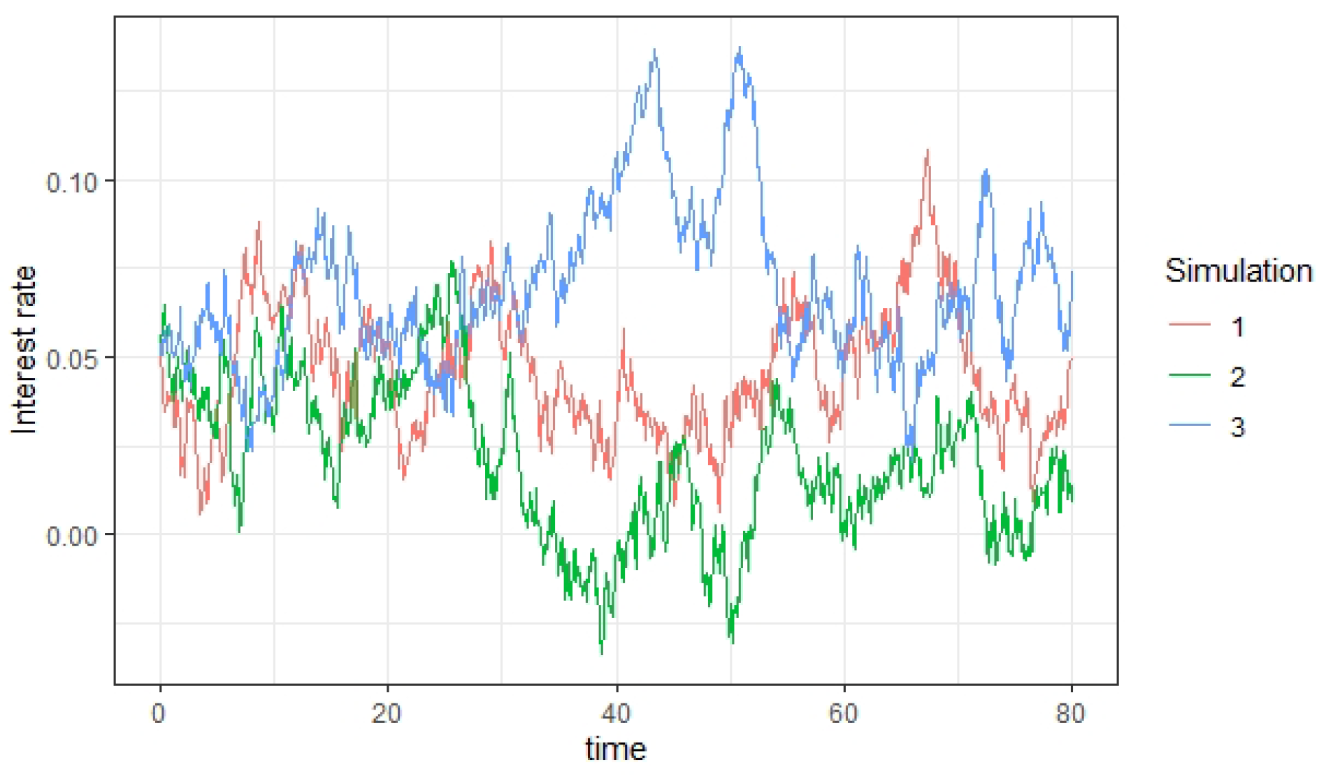
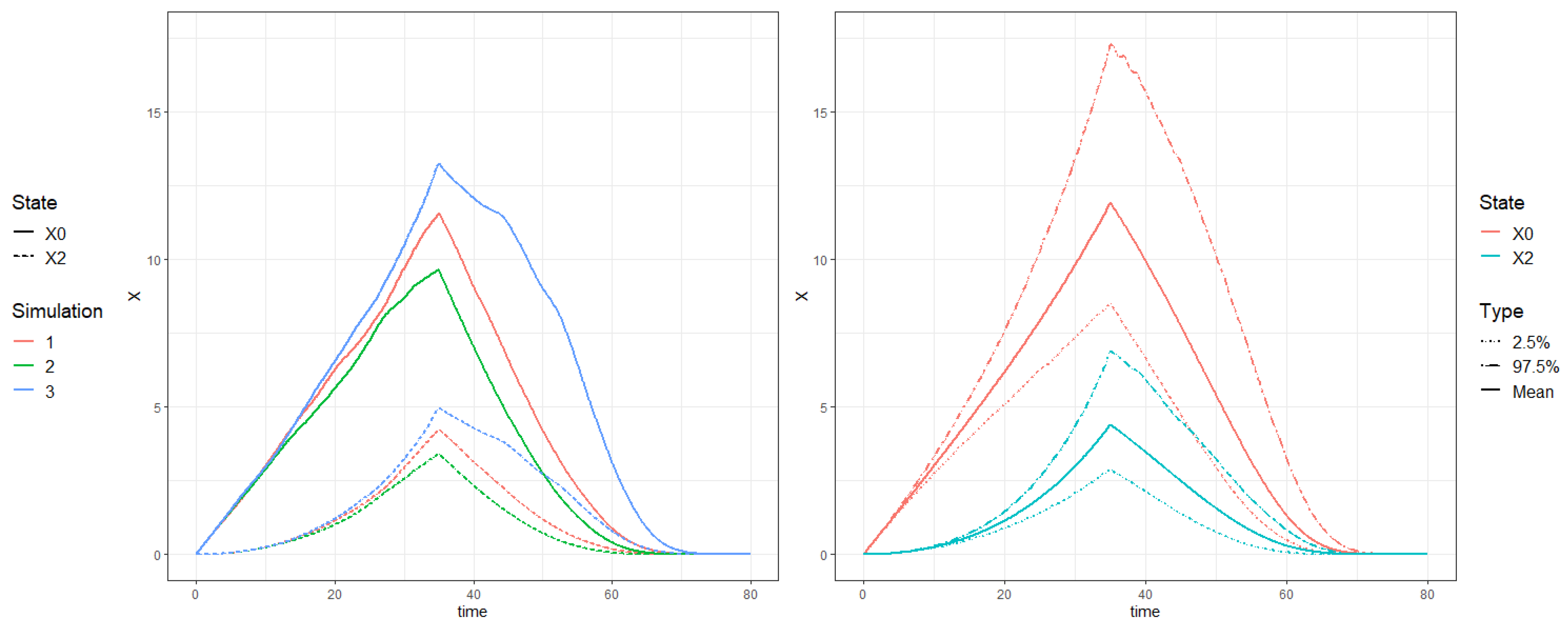
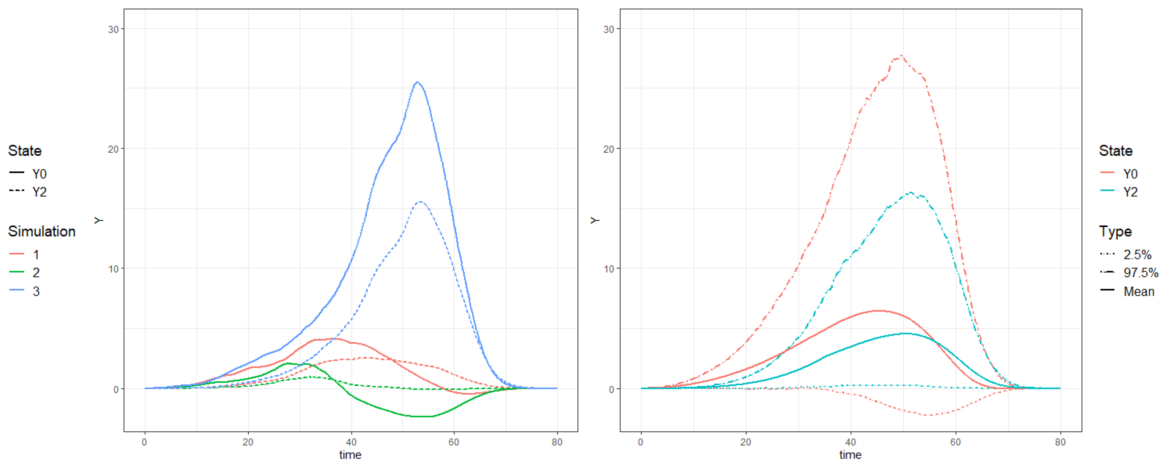
Figure 3 illustrates three simulated paths of the interest rate, simulated with an Euler scheme based on the dynamics of the interest rate. For each path of the interest rate, we project the savings account and the surplus in state 0 and 2 using Theorem 2 and illustrate the state-wise projections in Figure 4 (left) and Figure 5 (left).

The projected savings account is larger in state 0 than in the free-policy-state, since premiums cancel upon conversion to free-policy, which lowers the savings account. The interest rate impacts the projected surplus in Figure 5 (left) significantly. A high (low) interest rate results in a high (low) surplus contribution, which effects the projected surplus as illustrated in simulation 3 (2). A high interest rate results in high dividends in our numerical example; therefore, the projected savings accounts are highest in simulation 3. For the effects of changing the dividend strategy, see Bruhn and Lollike (2020). With these calculations, the insurance company can monitor the development of the insurance contract in various scenarios of the interest rate and, for instance, assess the effects of the chosen dividend strategy.

Based on 1000 simulations of the interest rate, we estimate the mean, the $2.5\%$-quantile, and the $97.5\%$-quantile of the projected savings account (see Figure 4 (right)) and the projected surplus (see Figure 5 (right)). This illustrates that within the Vasicek model with the chosen parameters and with the chosen dividend strategy, the $95\%$-confidence interval of the projected savings account is widest, when the insured retires at time 35, and the $95\%$-confidence interval of the projected surplus spans from $-2.2$ to $27.7$, which indicates to the insurance company that the development of the surplus is uncertain.

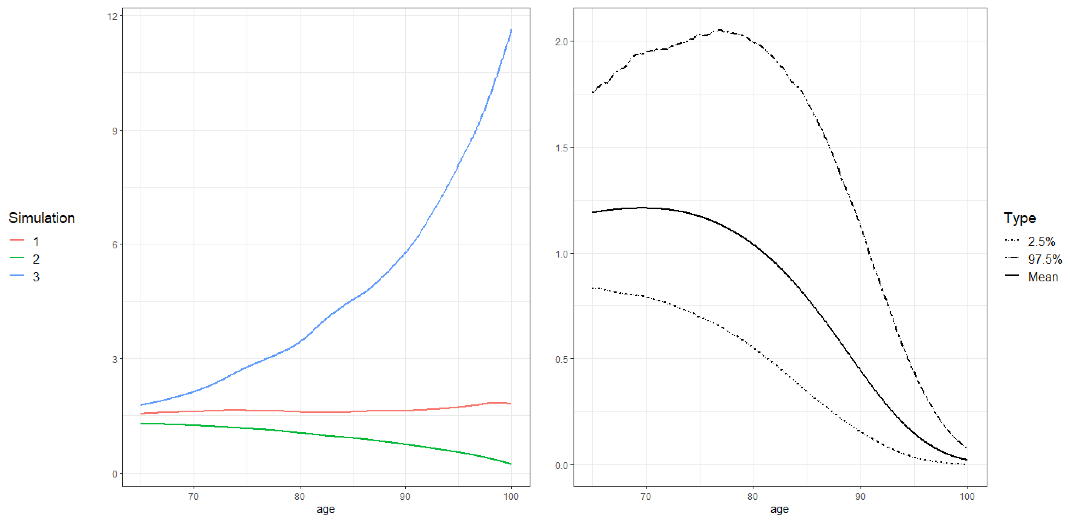
The insurance company is interested in communicating the expected life annuity payment to the insured, since it is regulated by bonus, and the amount of future bonus is unknown at initialization of the insurance contract. Figure 6 (left) illustrates the life annuity rate in the three simulated scenarios of the interest rate conditional on the insured being alive and in the non-free-policy state at the time of the payment. In scenario 3, the savings account is higher resulting in a high life annuity. Scenario 2 has a negative surplus due to a low interest rate, which results in negative dividends with the chosen dividend strategy; therefore, the life annuity gets below 1 in this scenario. At initialization of the insurance contract, the insurance company promises the insured a life annuity of 1 given alive and non-free-policy; hence, scenario 2 is bad for the company. The projection in Figure 6 (left) holds information to the insurance company that, when the interest rate is low, the insurance company should react and change their dividend strategy.

Figure 6 (right) illustrates the expected life annuity and a $95\%$ confidence interval of the life annuity as a function of age. The life annuity is weighted with the probability of dying and conversion to free-policy; hence, it is lower than the life annuity in Figure 6 (left), where we condition in being alive and non-free-policy.

7. Conclusions

The paper presents a method for projecting the savings account and the surplus of a life insurance contract including policyholder behavior in various financial scenarios. We present differential equations of the projected savings account and the projected surplus without policyholder behavior, which is the result of Bruhn and Lollike (2020). When including policyholder behavior, we cannot in general project the savings account and the surplus with an ideal free-policy factor using the methods from Bruhn and Lollike (2020).

In this paper, we show that, in the case where all benefits are regulated by bonus, we can actually find accurate differential equations for the state-wise projections of the savings account and the surplus with the ideal free-policy factor. We suggest an approximation to the ideal free-policy factor, and one of the main results is that, in the case where all benefits are regulated by bonus, the projections of the savings account and the surplus based on the ideal free-policy factor coincide with the projections based on the approximated free-policy factor. Therefore, we consider the approximated free-policy factor a reasonable approximation of the ideal free-policy factor.

We are able to project the savings account and the surplus with the approximated free-policy factor in a general case, and we present differential equations of the state-wise projections of the savings account and the surplus with the approximated free-policy factor. We consider this result as a key result in the projection of balances in life insurance and a good extension of Bruhn and Lollike (2020) to include policyholder behavior outside the case, where all benefits are regulated by bonus. We illustrate a numerical simulation example in three scenarios of the interest rate to highlight the practical application of our findings. This results in a projection of the savings account and the surplus for a chosen dividend strategy, which enables the insurance company to assess the effects of their chosen management actions. Furthermore, we study distributional properties of the projections.

This paper studies a simple dividend strategy which is linear in the savings account and the surplus. In order to use this model, insurance companies must choose their future dividend strategy according to this simple setup. Future research involves extending the model to include a more complex dividend strategy and allow for dependence of, for instance, assets, and market values. Another branch is the study of how to choose an optimal dividend strategy in this multi-state setup; see, for instance, Nielsen (2005).

References

- Ahmad, Jamaal, Christian Furrer, and Kristian Buchardt. 2020. Computation of bonus in multi state life insurance. arXiv arXiv:2007.04051. [Google Scholar]
- Asmussen, Søren, and Mogens Steffensen. 2020. Probability Theory and Stochastic Modelling. In Risk and Insurance. A Graduate Text, 1st ed. Cham: Springer International Publishing, vol. 96. [Google Scholar]
- Barsotti, Flavia, Xavier Milhaud, and Yahia Salhi. 2016. Lapse risk in life insurance: Correlation and contagion effects among policyholders’ behaviors. Insurance, Mathematics and Economics 71: 317–31. [Google Scholar] [CrossRef] [Green Version]
- Björk, Tomas. 2009. Arbitrage Theory in Continuous Time, 3rd ed. Oxford Finance Series. Oxford: Oxford University Press. [Google Scholar]
- Browne, Mark J., and Kihong Kim. 1993. An international analysis of life insurance demand. The Journal of Risk and Insurance 60: 616–34. [Google Scholar] [CrossRef]
- Bruhn, Kenneth, and Alexander Sevel Lollike. 2020. Retrospective reserves and bonus. Scandinavian Actuarial Journal, 1–19. [Google Scholar] [CrossRef]
- Buchardt, Kristian, and Thomas Møller. 2015. Life insurance cash flows with policyholder behavior. Risks 3: 290–317. [Google Scholar] [CrossRef] [Green Version]
- Buchardt, Kristian, Thomas Møller, and Kristian Bjerre Schmidt. 2014. Cash flows and policyholder behaviour in the semi-markov life insurance setup. Scandinavian Actuarial Journal 2015: 660–88. [Google Scholar] [CrossRef]
- Campbell, Ritchie A. 1980. The demand for life insurance: An application of the economics of uncertainty. The Journal of Finance 35: 1155–72. [Google Scholar] [CrossRef]
- Chen, Peng, Roger G. Ibbotson, Moshe A. Milevsky, and Kevin X. Zhu. 2006. Human capital, asset allocation, and life insurance. Financial Analysts Journal 62: 97–109. [Google Scholar] [CrossRef]
- Chiappori, Pierre-André, Bruno Jullien, Bernard Salanié, and François Salanié. 2006. Asymmetric information in insurance: General testable implications. The Rand Journal of Economics 37: 783–98. [Google Scholar] [CrossRef]
- Christiansen, Marcus C., and Boualem Djehiche. 2020. Nonlinear reserving and multiple contract modifications in life insurance. Insurance, Mathematics and Economics 93: 187–95. [Google Scholar] [CrossRef]
- De Giovanni, Domenico. 2010. Lapse rate modeling: A rational expectation approach. Scandinavian Actuarial Journal 2010: 56–67. [Google Scholar] [CrossRef]
- Henriksen, Lars, Jeppe Nielsen, Mogens Steffensen, and Christian Svensson. 2014. Markov chain modeling of policyholder behavior in life insurance and pension. European Actuarial Journal 4: 1–29. [Google Scholar] [CrossRef]
- Jensen, Ninna, and Kristian Schomacker. 2015. A two-account life insurance model for scenario-based valuation including event risk. Risks 3: 183–218. [Google Scholar] [CrossRef] [Green Version]
- Kraft, Holger, and Mogens Steffensen. 2008. Optimal consumption and insurance: A continuous-time markov chain approach. ASTIN Bulletin 38: 231–57. [Google Scholar] [CrossRef] [Green Version]
- Loisel, Stéphane, and Xavier Milhaud. 2011. From deterministic to stochastic surrender risk models: Impact of correlation crises on economic capital. European Journal of Operational Research 214: 348–57. [Google Scholar] [CrossRef] [Green Version]
- Nielsen, Peter Holm. 2005. Optimal bonus strategies in life insurance: The markov chain interest rate case. Scandinavian Actuarial Journal 2005: 81–102. [Google Scholar] [CrossRef]
- Norberg, Ragnar. 1991. Reserves in life and pension insurance. Scandinavian Actuarial Journal 1991: 3–24. [Google Scholar] [CrossRef]
- Norberg, Ragnar. 1999. A theory of bonus in life insurance. Finance and Stochastics 3: 373–90. [Google Scholar] [CrossRef]
- Richard, Scott F. 1975. Optimal consumption, portfolio and life insurance rules for an uncertain lived individual in a continuous time model. Journal of Financial Economics 2: 187–203. [Google Scholar] [CrossRef]
- Steffensen, Mogens. 2002. Intervention options in life insurance. Insurance Mathematics and Economics 31: 71–85. [Google Scholar] [CrossRef]
- Steffensen, Mogens. 2006. Surplus-linked life insurance. Scandinavian Actuarial Journal 2006: 1–22. [Google Scholar] [CrossRef]