Machine Learning in P&C Insurance: A Review for Pricing and Reserving


1
École d’actuariat, Université Laval, Québec, QC G1V 0A6, Canada
2
Département d’informatique et de génie logiciel, Université Laval, Québec, QC G1V 0A6, Canada
*
Author to whom correspondence should be addressed.
Risks 2021, 9(1), 4; https://0-doi-org.brum.beds.ac.uk/10.3390/risks9010004
Submission received: 30 October 2020
/
Revised: 19 November 2020
/
Accepted: 11 December 2020
/
Published: 23 December 2020
(This article belongs to the Special Issue Data Mining in Actuarial Science: Theory and Applications)
Abstract
:In the past 25 years, computer scientists and statisticians developed machine learning algorithms capable of modeling highly nonlinear transformations and interactions of input features. While actuaries use GLMs frequently in practice, only in the past few years have they begun studying these newer algorithms to tackle insurance-related tasks. In this work, we aim to review the applications of machine learning to the actuarial science field and present the current state of the art in ratemaking and reserving. We first give an overview of neural networks, then briefly outline applications of machine learning algorithms in actuarial science tasks. Finally, we summarize the future trends of machine learning for the insurance industry.
1. Introduction
The use of statistical learning models has been a common practice in actuarial science since the 1980s. The field quickly adopted linear models and generalized linear models for ratemaking and reserving. The statistics and computer science fields continued to develop more flexible models, outperforming linear models in several research fields. To our knowledge and given the sparse literature on the subject, the actuarial science community largely ignored these until the last few years. In this paper, we review nearly a hundred articles and case studies using machine learning in property and casualty insurance.
A case study comparing machine learning models for ratemaking was conducted by Dugas et al. (2003), who compared five classes of models: linear regression, generalized linear models, decision trees, neural networks and support vector machines. From their concluding remarks, we read, “We hope this paper goes a long way towards convincing actuaries to include neural networks within their set of modeling tools for ratemaking.“ Unfortunately, it took 15 years for this suggestion to be noticed. Recent events have sparked a spurge in the popularity of machine learning, especially in neural networks. Frequently quoted reasons for this resurgence include introducing better activation functions, datasets composed of many more images, and much more powerful GPUs LeCun et al. (2015).
Machine learning algorithms learn patterns from data. Linear regression learns linear relationships between features and a response variable, which may be too simple to reflect the real world. Generalized linear models (GLMs, also including logistic regression (LR)) add a link function to express a random variable’s mean as a function of a linear relationship between features. This addition enables the modeling of simple nonlinear effects. For example, a logarithmic link function produces multiplicative relationships between input features and the response variable. While these models are simple, easily explainable and have desirable statistical properties, they are often too restrictive to learn complex effects. Property and casualty insurance (P&C) covers risks that result from the combination of multiple sources (causes), including behavioral causes. Rarely will a linear relationship be enough to model complex behaviors. Nonlinear transformations and interactions between variables could more accurately reflect reality. To include these effects in GLMs, the statistician must create these features by hand and include them in the model. For example, to model a 3rd degree polynomial of a variable x, we would need to supplement and as new features. Creating these transformations and interactions by hand (a task called feature engineering) is tedious, so only simple transformations and interactions are usually tested by actuaries.
A first truly significant advantage of recent machine learning models simplifies the previous drawback: recent models learn nonlinear transformations and interactions between variables from the data without manually specifying them. This is performed implicitly with tree-based models and explicitly with neural networks.
The second advantage of machine learning is that many models exist for different types of feature formats. For instance, convolutional neural networks may model data where order or position is essential, like text, images, and time series of constant length. Recurrent neural networks may model sequential data like text and time series (think financial data, telematics trips or claim payments). Most data created today is unstructured, meaning it is hard to store in spreadsheets or other traditional support. Historical approaches to dealing with this data have been to structure them first (actuaries aggregate individual reserves in structured triangles). Much individual information is lost when structuring (aggregating). Many machine learning models can take the unstructured data directly, opening possibilities for actuaries to better understand the problems, data and phenomenon they study.
The field of machine learning is expanding rapidly and shows great promise for use in actuarial science. The introduction of machine learning in actuarial science is recent and not neatly organized: when reviewing the literature, we identified independent and exclusive contributions. In this review, we analyze and synthesize the work conducted in this area. For each topic, we present the relevant literature and provide possible future directions for research.
1.1. Research Methodology
We followed a structured methodology to search for contributions in this review. A three-pronged approach was used:
- Query research databases (Google Scholar, ProQuest, SSRN, arXiv, ResearchGate) for a combination of machine learning keywords (machine learning, data science, decision tree (DT), classification and regression trees (CART), neural network (NN) convolutional neural networks (CNN), recurrent neural networks (RNN), random forest (RF), gradient boosting (GBM/GBT/XGBoost), generalized additive model (GAM, GAMLSS), support vector machine (SVM, SVR, SVC), principal component analysis (PCA), autoencoders (AE), computer science) AND the subjects of interest in our review (actuarial science, general insurance, home insurance, auto insurance, P&C insurance, ratemaking, reserving).
- Query actuarial journals (in no particular order, Risks, ASTIN Bulletin, Insurance: Mathematics and Economics (IME), Scandinavian Actuarial Journal (SAJ), Variance, North American Actuarial Journal (NAAJ), European Actuarial Journal (EAJ)).
- For each pertinent article, we searched references therein for similar contributions.
In the introduction, we included publications classified as overviews.1 References for books and lecture notes are also included. These overview publications are often not peer-reviewed and do not propose new modeling approaches but provide empirical evidence or strategic plans that set the stage for research.
In the main review on reserving and ratemaking, we limited the contributions to articles in journals, conferences, and preprints. The time limit for research was August 2020. Although we do not have a beginning time limit, papers before 2015 are mainly included for historical context.
This review considered papers that have analyzed the topic of machine learning in pricing or reserving. Priority was given to models that adapted machine learning models to a specific insurance task. Due to the unique structure of reserving data, most contributions for reserving fit this criterion. We also included papers that have analyzed the topic of machine learning by justifying the use of a specific algorithm within a context or providing specific conclusions or model interpretations for the selected machine learning model. We read several papers where the authors proposed that a machine learning model could be used to perform a certain sub-task of a more significant process. Unless the model’s choice was justified, we did not consider these papers as part of this review.
We organize contributions with a thematic approach while using chronological ordering within themes.
1.2. Scope of This Review and Similar Work
In this paper, we review the literature on machine learning in P&C insurance. Due to the early stage of research, the literature is mostly composed of white papers and case studies. We include the works that have been useful to set the stage for research. Additionally, machine learning innovations are produced at a very high rate. This literature review contains some non-peer-reviewed works so that it is up to date with the current state-of-the-art.
In the past few years, efforts similar to ours include white papers, comparative studies, surveys from industry, and lecture notes. In Table 1, we summarize the aspects treated in each contribution.
Recent interest in predictive modeling in actuarial science has emerged, and Frees et al. (2014a) presented a survey of early applications of such models. The premise is encouraging: as data becomes more abundant and machine learning models more robust, insurers should have the capacity to capture most heterogeneity represented by insured individuals and compute a premium that represents their individual risk in a more accurate way.
We assume the reader is familiar with most statistical learning models such as GLMs, generalized additive models, random forests, gradient boosted machines, support vector machines and neural networks. Otherwise the reader is directed to Friedman et al. (2001) or Wuthrich and Buser (2019). The only model described in this review is the neural network since we believe it is underrepresented in actuarial science. Many white or review papers reflecting on the use of big data and machine learning in actuarial science are available, we highlight Richman (2020a, 2020b) (with a focus on deep learning). The ASTIN Big Data/Data Analytics working party published Bruer et al. (2015), composed of a collection of ideas concerning the direction of data analytics and big data, which our paper wishes to update five years later. Another work related to this paper but with a wider (but less specific) scope is Corlosquet-Habart and Janssen (2018), who collected high-level ideas of the use of big data in insurance. They present general machine learning techniques, while our goal is to present machine learning applications in actuarial science. In Grize et al. (2020), the authors present case studies on car insurance and home insurance pricing. We highlight the 6th section of that paper, enumerating several challenges for the insurance industry, including establishing a data-oriented company culture, continuing education and ethical concerns, including fairness and data ownership. We expand on the issue of fairness later in this paper.
Professional organizations have also shown great interest in machine learning and big data by creating working parties and calls for papers. The working group, “Data Science” of the Swiss Association of Actuaries, has recently published a series of tutorials to offer actuaries an easy introduction to data science methods with actuarial use, see Noll et al. (2018), Ferrario et al. (2018), Schelldorfer and Wuthrich (2019), Ferrario and Hämmerli (2019) and others. The Casualty Actuarial Society (CAS) had a data and technology working party who published a report Bothwell et al. (2016). The Institute and Faculty of Actuaries set up the Modelling, Analytics and Insights in Data working party and published their conclusions in Panlilio et al. (2018). The Society of Actuaries sponsored a survey of machine learning in insurance in Diana et al. (2019). The Society of Actuaries and the Canadian Institute of Actuaries sponsored a survey of predictive analytics in the Canadian life insurance industry Rioux et al. (2019). The Society of Actuaries also published a report on harnessing the new sources of data and the skills actuaries will need to deal with these new issues2. Actuarial research journals have also been announcing special issues on predictive analytics, for example, Variance3 and Risks.4
1.3. Generalized Data on This Review
To provide an overall view of the research, we provide generalized data of papers covered in the review. Figure 1 presents a breakdown of the 77 publications by year since 2015 (among the contributions in Table 1, Table 2, Table 3 and Table 4). The increasing trend shows how current this subject is. Note that 2020 data are limited to August. We observe that pricing has started using machine learning before reserving because the research context is already familiar with pricing using generalized linear models. Reserving, being an unstructured source of data is less straightforward, but the number of publications using machine learning has increased in the past two years.
Figure 2 presents the number of publications by source (among the contributions in Table 2, Table 3 and Table 4). Journals with a single paper were grouped in Other and mainly consisted of pricing. The categories of journals included in Other are business, statistics, expert systems, finance.
Finally, the distribution of model families is presented in Figure 3 (among the contributions in Table 2, Table 3 and Table 4). In our experience and after analyzing the best models in competitions hosted on Kaggle, decision tree ensembles work best for structured problems, while neural networks work best for unstructured problems. This is in line with the breakdown of models in this review: pricing uses structured data and boosting (XGBoost, GBT) is the most popular pricing framework, while reserving uses unstructured data (due to the triangular format of aggregated reserves or the time series format of individual reserves) and neural networks are the most popular for reserving models. We believe that GAMs are popular for pricing since actuaries are already familiar with generalized linear models, and GAMs are generalizations of GLMs.
The remainder of the paper is organized as follows. In Section 2, we briefly introduce neural networks and present two methods to estimate the parameters of a probability distribution. Section 3 covers machine learning applications to ratemaking, while Section 4 covers their applications to reserving. Section 5 concludes the review by summarizing the future trends and challenges using machine learning in insurance.
2. Neural Networks
In this section, we present a brief introduction to fully connected neural networks. We also present how to estimate the parameters of random variables with this model.
Neural networks construct a function f such that , where corresponds to the features in the model, is a response variable and are model parameters. This function is built as a composition (aggregation) of functions (layers)
In this case of 3 chained functions, corresponds to the first layer, to the second layer and to the third layer. Since we are not interested in the first or second layers’ output, we call these hidden layers. The last layer is called the output layer since this is the output of the classification or regression model. The number of chained functions is called the depth of the model. Each function is nonlinear; composing multiple functions produces a highly nonlinear model, thus having much flexibility to estimate the function f.
2.1. Basics and Notation
Let be the p-dimensional features for observation i inputted into the neural network. We define the first hidden layer as
with
where is the width of the first hidden layer, is a nonlinear function called the activation function. If the width is equal to 1 and the activation function g is the sigmoid function
(sometimes noted ), we recognize the inverse link function in the logistic regression. However, we could use the hidden layer values as input variables in another function. The second hidden layer values are
with
where is the width of the second hidden layer, and is the second activation function. We may then repeat this process for L layers, where values of the hidden layer are
with
and
where is the output size. In Figure 4, we present the graphical diagram for a neural network with two hidden layers. Here, which is often the case in practice but does not need to be. Usually, for regression, such that the model predicts a single value and can be interpreted as the GLM link function. In other cases, notably when the neural network predicts the parameters of a probability distribution, will correspond to the number of parameters that define the random variable. We will return to this in Section 2.2.
Along with the sigmoid function defined in (4), popular choices of activation (nonlinearity) functions are the hyperbolic tangent (tanh), given by
and the Rectified Linear Unit (ReLU), defined by
We briefly reviewed neural networks in this section, but interested readers may refer to Goodfellow et al. (2016) for a comprehensive overview of the field.
Neural networks may be used in regression tasks and classification tasks. For regression, there is a single output value representing the prediction. To better illustrate this idea, we present the link between neural networks and GLMs. The prediction formula for a GLM is
A neural network with no hidden layer and one output neuron corresponds to a GLM. This process is shown in Figure 5. In neural network graph notation, each node (other than in the input layer) implicitly contains an activation function, omitting to draw a node for g. Each arrow between nodes has a weight, and the bias is also assumed.
Therefore, a neural network with many hidden layers may be viewed as stacked GLMs. Each hidden layer adds nonlinearity and can learn complex functions and nonlinear interactions between input values. We may interpret the output layer as a GLM on transformed input variables, where the model learns the necessary transformations, performing automatic feature engineering.
A significant drawback of neural networks is that they are black boxes and offer minimal theoretical guarantees. In order to perform risk management, we also need a probability distribution. The next subsection presents how to estimate parameters of a probability distribution with neural networks.
2.2. Estimating Probability Distribution Parameters with Neural Networks
Most data scientists fitting neural networks for regression use a mean squared error loss function, and the output of the network is the expected value of the response variable. The two drawbacks to this approach are that (1) the mean squared error assumes a normal distribution, and (2) there is no way to quantify variability. Instead of directly predicting the outcome, we propose estimating the random variable parameters directly, surmounting these drawbacks.
Let us first consider a discrete response variable and assume that the Poisson distribution is appropriate, as in Fallah et al. (2009). Let n represent the number of observations in the training dataset. The output of the neural network is the intensity parameter . The exponential function is the logical choice for the final activation function such that the intensity parameter is positive. The loss function is the negative log-likelihood, proportional to
See Figure 6a for a graphical representation of a network with one hidden layer.
Another method to estimate parameters of exponential family (EF) distributions with neural networks is presented in Denuit et al. (2019a). Exponential family distributions have a probability density function of the form
with . The mean and variance are respectively given by
and
The loss function is the unscaled deviance. In this approach, the neural network is designed to estimate only the mean parameter , see Figure 6b. For distributions with two parameters (gamma, normal), we obtain the second parameter using the method of moments method with the statistic:
where n is the number of observations used to train the model, and m is the number of parameters in the model. We note that neural networks often have a high number of parameters, so the denominator may be large (or negative if ).
The difference between models in Figure 6a,b is that the first model estimates the parameter of the Poisson distribution, while the second model predicts the mean of the random variable. We note that due to the nonconvexity of loss functions in neural networks, the solutions will be different unless the predicted parameter corresponds to the random variable’s mean.
For distributions outside the exponential family or when the number of parameters in the neural network is high, another technique is preferable to estimate distribution parameters. We generalize the neural network presented in Fallah et al. (2009). In this approach, the output of the neural network corresponds to the parameters of the distribution, and the loss function is the negative log-likelihood (NLL) of observations
In Figure 7a, we present a negative binomial neural network, where the output of the network is the two parameters of the model. The r parameter must be positive, so this parameter’s activation function could be the exponential function. The p parameter has a domain so that we can use a sigmoid activation function. The Tweedie distribution, important in actuarial science, can also be trained using a neural network. The output of the network corresponds to the distribution’s three parameters, see Figure 7b. Since the domain for every parameter is the positive real numbers, we can use the exponential activation function for each output neuron.
3. Pricing with Machine Learning
This section provides an overview of machine learning techniques for actuarial a priori pricing (also referred to as ratemaking or setting tariffs). The objective in pricing is to predict future costs associated with a new customer’s insurance contract with no claim history information for this customer. Since GLMs are current practice, we do not cover contributions using this method. We first present pricing with conventional features, followed by neural pricing. These contributions are summarized in Table 2. Then, we present a brief overview of telematics pricing with machine learning and conclude with an outlook on the pricing literature. Contributions for conventional pricing and telematics pricing usually apply the methods to auto insurance datasets.
3.1. Conventional Pricing
Generalized linear models aim to establish a relationship between variables and the response by combining a link function and a response distribution. This relationship is determined by the GLM score, the linear relationship between variables and regression weights. The linear relationship may be too restrictive to model the response distribution adequately. GAMs and neural networks offer solutions by adding flexibility to the score function. Another popular approach for pricing is using tree-based methods, which often surpass other algorithms for regression tasks. Since a priori pricing is a straightforward regression task, actuaries may use most regression models like GLMs, tree-based models and neural networks.
We start this section by presenting the frequency models. In Christmann (2004), the probability of filing m claims is modeled by
where is predicted with a logistic regression and is modeled with a support vector regressor.
Another method to perform frequency modeling is by considering frequency not as a discrete random variable but as a class to predict. This approach is used in Liu et al. (2014), using the support vector classifier. In a similar spirit, So et al. (2020) presented a multiclass Adaboost algorithm to classify the number of claims filed in a period. This new algorithm is capable of handling class imbalance (a large proportion of zero claims). We note that these approaches treat a regression task as a classification task, classifying discrete counts instead of a discrete probability distribution. This approach is rare in practice, but see Chapter 4 of Deng (1998) or Salman and Kecman (2012) for examples where this technique works well.
The main disadvantage of the three frequency models is that predictions are deterministic, meaning that a single value is predicted instead of a distribution. This approach is not frequently used in actuarial science since a distribution is useful for diagnosing model accuracy and calculating other actuarial metrics.
The remaining papers in this subsection deal with total costs associated with an insurance contract. Generalized additive models in insurance academia were first studied by Denuit and Lang (2004) and revisited with GAMLSS in Klein et al. (2014). This model was also used in actuarial ratemaking by Henckaerts et al. (2018), who employed generalized additive models to discover nonlinear relationships in continuous and spatial risk factors. Then, these flexible functions are binned into categorical variables and used as a variable in a GLM. GAMs also appear in telematics pricing in Boucher et al. (2017), who explored the nonlinear relationship between distance driven or driving duration and claim frequency.
A modification of the regression tree is presented in Paglia and Phelippe-Guinvarc’h (2011) to adjust for exposures different than one. Instead of dividing total claims by the exposure to return to the unit exposure base, the offset is incorporated in the deviance function, which served as a splitting criterion.
Gradient boosting is applied to prediction of at-fault accident loss costs in Guelman (2012). Multivariate decision trees are applied in Quan and Valdez (2018) to model the joint distribution of response variables in multiple coverages. Extensions to random forests and gradient boosting are also presented. The TDboost algorithm is presented in Yang et al. (2018). This algorithm uses gradient boosting to estimate the parameters of a Tweedie distribution. As opposed to the XGBoost framework, explicit update formulas are established from the profile likelihood. Important interactions are identified using partial dependence plots. A zero-inflated variant is presented in Zhou et al. (2020). Then, Henckaerts et al. (2020) compared GLM, GAM, trees and gradient boosting machine to predict future costs associated with an insurance contract. Many methods of variable importance and interpretability are applied, a crucial step in insurance pricing. To extract interactions, they applied Friedman et al. (2008).
In Lee and Lin (2018), a boosting algorithm is presented. The original gradient boosting is based on three actions: a basis, a regression and an adjustment. The delta boosting machine is proposed, combining the regression and adjustment steps. Therefore, the algorithm is said to be computationally efficient. Algorithms for distributions in the Tweedie family are presented, and the model is applied to car insurance claims data.
Then, Diao and Weng (2019) presented the regression tree credibility model, a tree-based method for pricing with credibility theory. The classic Bühlmann–Straub credibility premium is applied within each tree terminal node. To our knowledge, this is the only contribution using machine learning for a posteriori pricing.
A model capable of performing variable selection, such as elastic-net, for multiple response variables with a Tweedie distribution, is presented in Fontaine et al. (2019). A multitask regression model selects variables useful for many regression tasks, so useless variables are less likely to be retained. The proposed algorithm updates weights via the proximal gradient descent scheme to update model coefficients.
Mixture of experts or model averaging are other flexible approaches to insurance pricing. Since these methods are not machine learning but statistical, we do not investigate further but highlight Fung et al. (2019a, 2019b); Hu et al. (2018, 2019); Jurek and Zakrzewska (2008); Počuča et al. (2020); Richman and V. Wüthrich (2020); Ye et al. (2018). See Fung et al. (2020) for an application in reserving.
3.2. Neural Pricing
Early attempts of applying neural networks for insurance pricing include Lowe and Pryor (1996), Pelessoni and Picech (1998), Speights et al. (1999) and Francis (2001). Neural networks are also used in Chapados et al. (2002), who compared statistical learning models for estimating the pure premium. They also compared support vector regression but concluded that their predictive performance is not good since data are asymmetric, and the model must be overfitted to learn something useful. A fairness criterion is then defined to ensure the pure premium does not systematically discriminate against a specific group in the population.
A neural network is used to predict a posteriori frequency in Sakthivel and Rajitha (2017). The model input is historical claim frequency for a contract, along with the credibility factor and estimated annual claims frequency calculated using Bayesian credibility theory. The model output is the estimated annual claims frequency for the following year.
The adversarial variational Bayes method is used to model a Tweedie distribution with mixed models in Yang et al. (2019). Parameters of this distribution are optimized using adversarial variational Bayes, minimizing the Kullback–Leibler divergence with a variance reduction technique to stabilize gradients.
An interesting model proposition is the Combined Actuarial Neural Net (CANN) approach of Wuthrich (2019); Wüthrich and Merz (2019), where a neural network is used to model nonlinear relationships that were not captured by a simpler model. An example CANN model could be starting with a GLM to estimate
Then, the GLM coefficients are estimated. This task is repeated with a neural network to estimate
Finally, the two regression functions are added
We can interpret the GLM as a skip connection to the fully-connected neural network. In reality, the GLM predicts the pure premium, and the neural network adjusts for nonlinear transformations and interactions that the GLM could not capture. We can therefore interpret the original GLM parameters, partially explaining the final prediction.
While neural network predictions may be accurate at the policyholder level, it may not be at the portfolio level. This goes against an actuarial pricing principle Casualty Actuarial Society, and Committee on Ratemaking Principles (1988), which states, “A rate provides for all costs associated with the transfer of risk,” meaning that equity among all insured in the portfolio is maintained. Wüthrich (2019) proposed two methods that address this issue. The first uses a GLM step to the gradient descent method’s early stopped solution because GLMs are unbiased at the portfolio level. The other is to apply a penalty term in the loss function.
Machine learning models require large datasets. Publicly available datasets for insurance pricing are few, making research with complex models difficult. Generating synthetic datasets keeping the risk characteristics but removing confidential information is therefore important. Kuo (2019b) presented a model based on CTGAN to synthesize tabular data, and Côté et al. (2020) compared additional approaches.
3.3. Telematics Pricing
Telematics data is one of the first unstructured data sources to be extensively used in insurance pricing since it provides a better exposure base. This data source enables Pay-As-You-Drive insurance, where the premium is a multiple of the vehicle (in the distance or duration). A more recent innovation is the Pay-how-you-drive insurance model, where surcharge or discounts are applied based on driving behavior. An early survey of telematics use in insurance companies is presented in Yao and Katz (2013).
Telematics data are highly voluminous and unstructured, two situations where flexible algorithms have high predictive performance. For this reason, many models for telematics pricing are based on machine learning. Table 3 presents a summary of telematics models using machine learning.
3.3.1. Pay-as-You-Drive
A pure premium should represent the expected loss for an insurance contract to an exposure. An example of such exposure could be the value of the insured good, since if the value of materials doubles, the insurance contract should, in principle, also double. When pricing a contract, we must define an exposure base. According to Werner and Modlin (2010), a good exposure base should
- be proportional to the expected loss;
- be practical (objective and inexpensive to obtain and verify);
- consider preexisting exposure base established within the industry.
Indeed, car insurance has, for a long time, been based on car-years insured. While reported kilometers-driven is often used as a rating variable, it is not always used as an exposure base since it is expensive to verify (and simple for the insured to provide false information). The use of telematics data to investigate alternative exposure bases was done in Boucher et al. (2013), who showed that the relationship between annual driven kilometers and the frequency of claims was not linear, concluding there is a reduced risk of accidents as a result of experience. The relationship has been modeled individually with the use of GAMs in Boucher et al. (2017), so these variables may not be used as exposure bases (offsets, in a linear or additive model). However, they must be considered a rating variable to capture the pure premium relationship fully. Then, Verbelen et al. (2018) combines policy information with telematics information with a GAM model and the models which include both types of data have a better regression performance on most criteria. Telematics data have also enabled different statistical distribution assumptions based on the usage of the vehicle. For example, Ayuso et al. (2014) analyzed the time between frequency claims based on distance.
3.3.2. Pay-How-You-Drive
In traditional non-life insurance ratemaking, an issue with providing an adequate premium for the risk is that losses associated with contracts may take time to manifest. For example, a hazardous driver may be fortunate and have no accident, while a skilled and alert diver may experience bad luck and get involved in an accident rapidly. It was impossible to differentiate between the driving styles and many years of experience (along with credibility theory), leading an actuary to price a contract for the risk accurately. The use of variables describing the driving context (for instance, road type or acceleration tendencies) is a groundbreaking solution since this data may rapidly provide insights on driving behavior. Thus, individuals with the same classical actuarial attributes may be priced differently according to the insured driving style through the data collected from telematics devices Weidner et al. (2017).
We are currently in a stage where the velocity and volume of telematics data are hard to manage since actuaries are not historically equipped with the computer science skills associated with dealing with such data. Additionally, the little available data are sometimes not accompanied by claims data, meaning it is challenging to validate if a driving style is riskier or safer. For example, one could think that an individual with hard breaking tendencies represents an increased probability of an accident. However, this individual may have higher reflexes enabling him to make such adjustments rapidly. To our knowledge, some insurance companies consider hard breaks as accidents. The reason is that hard breaks occur during accidents or near-misses, so any insured performing a hard break had or almost had an accident. This hypothesis increases accident frequency in the dataset, potentially leading to better model performance. Since the study of telematics data is in its infancy, such expert knowledge hypotheses must be made.
However, there have been some efforts to summarize driving behaviors in the actuarial literature. Weidner et al. (2016) presents a method to build a driving score based on pattern recognition and Fourier analysis. Then, a solution to the small number of observations was proposed by Weidner et al. (2017), who used a Random Waypoint Principle model to generate stochastic simulations of trip data, under constraints, such as speed limits, acceleration and brake performance. A clustering analysis based on medians of speed, acceleration and deceleration is performed to create classes of trips. Then, the few trip data available can be associated with each class.
Another approach to summarize driving styles was proposed by Wüthrich (2017) through the use of velocity–acceleration heatmaps. These heatmaps are generated for different speed buckets to represent the velocity and acceleration tendencies of drivers. Then, the k-means algorithm is applied to create similar clusters of drivers. Note that contrarily to Weidner et al. (2017), these heatmaps are generated by drivers and not by trips, meaning a change in drivers is an issue with this approach. This idea is followed by Gao and Wüthrich (2018), who use Principal Component Analysis and autoencoders to project the velocity-acceleration heatmaps in a two-dimensional vector that can be used as part of rating variables.
In Pesantez-Narvaez et al. (2019), logistic regression is compared to gradient boosting to predict the occurrence of a claim using telematics data. They conclude that the higher training difficulty associated with XGBoost makes this approach less attractive than logistic regression.
A study by Gao and Wüthrich (2019) examined the use of convolution neural networks in classifying a driver based on the telematics data (speed, angle and acceleration) of short trips (180 s). Classification results were encouraging, but only three drivers could be modeled at once due to the small volume of data.
As previously stated, clustering or classification models are hard to evaluate since researchers may have access to telematics data but not the claims data associated with these trips. Therefore, it is up to the actuaries’ domain knowledge to adapt the insurance premium based on identified clusters’ characteristics. Additionally, the models proposed do not contextualize the data, meaning the surrounding conditions that caused the driving patterns (speed limits, weather, traffic, road conditions) are not used when classifying the drivers. More recently, Gao et al. (2018) and Gao et al. (2019) proposed a GAM Poisson regression model that provides early evidence of the explanatory power of telematics driving data. Then, Gao et al. (2020) provided empirical evidence that using velocity-acceleration heatmaps in convolutional neural networks improves pricing.
The clustering and creation of driver scores is a branch of transportation research (see Castignani et al. (2015); Chen and Chen (2019); Ferreira et al. (2017); Wang et al. (2020)). We highlight Narwani et al. (2020), who presented a driver score based on a classification of the presence of claim and k-means clustering with similar drivers.
3.4. Outlook on Pricing
Telematics pricing is a new problem in actuarial science since data are only available recently. As the industry begins to share data with researchers, there is enormous potential for this technology in the pricing literature. There is a gap in the literature for feature engineering with pay-how-you-drive models. In our conversations with insurers and after surveying the literature, expert priors (like velocity-acceleration heatmaps or number of hard breaks) are the preferred methods used in practice and research to model telematics trips. We believe that recurrent neural networks will provide more insights into driving patterns but have not found any literature on the subject. Actuarial science researchers could also look at autonomous driving models — sometimes based on deep reinforcement learning — to model driver behavior.
Finally, actuaries must be conscious of the debate on insurance fairness in science and technology studies (STS), political science and sociology of markets. Insurance is becoming individualized or personalized due to increased predictive abilities (machine learning) and more data (telematics, wearable technology and smartphone sensors). This questions the role of insurance in society, transitioning from pooling risks (wealth redistribution) to the transfer of individual risks by paying a premium proportional to the actual hazard. See Barry (2019); Keller et al. (2018); Frezal and Barry (2019); Barry and Charpentier (2020); Cevolini and Esposito (2020) for an overview of this debate.
4. Reserving with Machine Learning
This section reviews the contributions to the actuarial science literature that use machine learning for reserving. While the link between regression and a priori ratemaking is straightforward, it is not for reserving. Thus, actuaries must modify the machine learning algorithm to fit reserving data or modify reserving data to fit structured datasets for regression. Reserving is a time series forecasting problem, see Benidis et al. (2020); Lim and Zohren (2020) for recent reviews on forecasting with machine learning. We say that the total reserve (Tot Res) is the sum of the reported but not settled (RBNS) reserve and the incurred but not reported (IBNR) reserve. We also note that the overdispersed Poisson model (ODP) and chain ladder (CL) can model total, RBNS or IBNR. An overview of contributions using machine learning for reserving with aggregate (Agg) and individual (Ind) data is presented in Table 4.
4.1. Aggregate Reserving
Reserving data is unstructured: since the number of payments and the time until a claim closes are unknown at the time of reporting (or at a certain valuation date), we may not store individual claims neatly in spreadsheets. For this reason, actuaries classically aggregate claim information in two ways:
- aggregation of multiple claims at the portfolio level or other grouping types if the actuary believes that development patterns are heterogeneous within the portfolio;
- aggregation of continuous-time into interval time, usually yearly, quarterly or monthly.
The usual aggregate reserve strategy is to estimate loss development factors (LDFs) to project the reserve at a particular period to the next period. The LDFs are determined as averages of age-to-age factors of observations split in accident year/development year triangles.
Let be the incremental claims amount for accident year and development year , where are optional regression parameters. Let be the loss development factor for period j. The Mack chain ladder assumption is
Many nonparametric models for aggregate reserving have been proposed, such as GAMs England and Verrall (2001). The incremental paid claims is modelled with a GAM, where
and
where are offsets, represents an inflation term. Smooth spline terms are for accident years and for development years. An extension to GAMLSS (with distribution other than the one-parameter exponential family) is then presented in Spedicato et al. (2014).
In Lopes et al. (2012), a two-stage procedure is proposed for estimating IBNR values. The first step consists of calculating chain ladder estimates of IBNR values, and a section step applies SVR and Gaussian process regression to residuals of the first model.
4.2. Neural Aggregate Reserving
An extension of chain ladder reserving is offered in Wüthrich (2018b), who models development factors with a shallow neural network. The loss function is a weighted square loss (with positive observed claims) given by
When ignoring attributes from x, the loss function becomes the Mack CL model. In Gabrielli et al. (2019), the cross-classified over-dispersed Poisson reserving model is generalized to neural networks. This enables more flexibility, including the joint modeling of claims triangles across different lines of business. This idea is expanded to the joint development of claim counts and claim amounts in Gabrielli (2020b). A more general ODP model is presented in Lindholm et al. (2020), which uses regression functions like GBM and NN.
Recurrent neural networks are neural networks capable of dealing with sequential data. Therefore, they are well suited for reserving tasks. This model is examined in Kuo (2019a) for aggregate triangles. Aggregate loss experience data for subsequent is fed to a recurrent neural network layer. Company information is fed to an embedding layer.5 Both layers are combined with fully-connected layers to predict claims outstanding and paid loss.
4.3. Individual Reserving
With individual reserving, actuaries may observe individual claims (removing the aggregation within the portfolio). This is also called triangle-free reserving or granular reserving. The advantage is twofold. First, the reserving model may depend on the claim’s characteristics that may impact its development pattern, for instance, line of business, injury part, and age of the claimant. Second, actuaries may model individual events within a claim. For instance, in discrete time individual reserving, predicted values may include
- claim status (open, close, reopen), a classification task;
- activity status (presence of claim or change in case reserve indicator during the period), a classification task;
- individual payment value or change in case reserve value conditional on the presence of claim during the period, a regression task;
- involvement of lawyers or doctors, a classification task.
Some individual reserving models also deal with claims continuously (removing the aggregation within periods). Since individual reserving is useful for following individual claims, these models usually focus on RBNS claims and use aggregate methods for IBNR claims.
Machine learning methods have rapidly become a methodology of choice for the analysis of individual reserves. The use of neural networks for individual reserving dates back to Mulquiney (2006), extending the previous state-of-the-art GLM reserving models. See Taylor (2019) for a recent review of reserving models.
Individual reserving brings up new challenges for actuaries. First, this approach requires dealing with two types of data. In Taylor et al. (2008), the notion of static variables and dynamic variables is brought up. Static variables remain constant over the claim settlement process, while dynamic variables may change over time. For example, the gender of the client will most likely remain the same, while the client’s age will evolve for claims spanning over one year. Another example of dynamic variables is the claims paid and a variable indicating if a claim is open or closed. Reserving models need to deal with dynamic variables since we try to model payments over time, and variables often change in time. The paper goes on to propose a few parametric individual loss reserving models.
Public individual claims data may be difficult to obtain for researchers. In this situation, simulation offers a great way to generate anonymized individual claims histories and attributes. Such a model is offered in Gabrielli and Wüthrich (2018)6, who train a neural network to predict individual claim histories based on a risk portfolio. For every claim, we have individual characteristics that models may use as input variables. A sequence of claim amounts and closed/open status for each claim is available for every development year (for a maximum of 12 years). This simulation machine produces observations at the individual level but time-aggregated to periods of one year (for this reason, continuous models are not appropriate for this type of data). Many of the contributions of this section use this simulation machine as applications of individual reserving models.
A flexible method for applying machine learning techniques in individual claims reserving is proposed in Wüthrich (2018a). Only regression trees are considered in the paper, and only the number of payments is modelled, although actuaries may scale the approach to other applications. Regression trees are used to model a claim indicator and a close indicator, using variables from initial claim information and past payments. Llaguno et al. (2017) expand this model by removing the reliance on dynamic variables with clustering, and De Felice and Moriconi (2019) consider frequency and severity components.
One problem in reserving is that claims that take more time to develop are usually more expensive (and short settling times are usually associated with smaller claim amounts). When building a reserving model with a particular valuation date, we include a higher proportion of smaller claims than reality. The complete claims history of short settling times is included in the dataset, but only partial claim histories of longer developing claims. This is a problem of right censoring, and Lopez et al. (2016) presents a modified weighted CART algorithm to take this into account. Lopez et al. (2019) use weighted CART as an extension of Wüthrich (2018a). See also Lopez and Milhaud (2020) for an alternate approach to loss reserving using the weighted CART.
The gradient boosting algorithm is applied in Pigeon and Duval (2019), using individual reserving claim histories to predict the total payment. The paper provides multiple approaches for dealing with incomplete (undeveloped) data. Since complete claim histories are needed to train the model, underdeveloped claims are completed using aggregate techniques such as Mack or Poisson GLM. Bootstrap is applied to complete triangles, so the variance of final reserves isn’t underestimated. Variables are used in the model, such as age, but not in the gradient boosted tree, only as variables in the Poisson GLM. The case study in this paper is useful for practitioners since many hypotheses are compared and validated.
A creative approach for individual claims reserving was proposed by Baudry and Robert (2019). Although machine learning contributions are not the focus of the paper, the train and test database building provides future researchers with the opportunity to deal with individual claims data with many kinds of machine learning models.
Another approach to reserving is clustering observations into homogeneous groups. Carrato and Visintin (2019) explains how to use the chain ladder method for individual data. They then propose clustering observations based on static variables like the line of business and dynamic variables like payment sequence. Then, they construct a linear chain ladder model for each cluster.
Finally, we highlight Crevecoeur and Antonio (2020), who present a hierarchical framework for working with individual reserves. The likelihood function for RBNS is decomposed into temporal dimensions (chronological events) and event dimensions (called update vectors, composed of distributions for a payment indicator, a closed indicator and a payment size). The framework allows for any modeling technique at each layer, so actuaries may use machine learning algorithms to model the three event types (the paper uses GLMs and GBMs). Additionally, many aggregate reserving models can be restated as hierarchical reserving models.
4.4. Neural Individual Reserving
The simulation machine is used in Gabrielli et al. (2019). When only one aggregated claims triangle is available, a machine learning algorithm cannot be trained. To create many triangles, individual claim histories are split in a train and test dataset, and aggregated triangles are build using the subset of claim histories. They then apply a neural network to predict the total reserve.
An individual claim reserving model is presented in Delong et al. (2020). The reserving task is broken down into six steps, and a neural network is trained for each task: modeling IBNR counts, payment status process of RBNS claims, an indicator of RBNS recovery claims, expected claim and recovery payments of RBNS claims, an indicator of IBNR with no payment, and claim amounts of nonzero IBNR claims.
In Gabrielli (2020a), the RBNS prediction task is separated into sub-networks. For each possible development period, a sub-network predicts the type of payment (classification task) and the mean parameter of a log-normal distribution for the amount of payment. This network leverages parameter sharing, a principle of multitask learning that generalizes features learned in the network.
An individual claims model for RBNS claims using recurrent neural networks is introduced in Kuo (2020). The author uses an encoder LSTM for past cash flows and claim status sequences and a decoder LSTM to generate a paid loss distribution. Also, a Bayesian neural network at the output of the decoder enables uncertainty quantification.
4.5. Outlook on Reserving
While several researchers proposed models for aggregate reserving with machine learning, most of these approaches build separate runoff triangles for every set of variables (or cluster of similar attributes). When actuaries aggregate reserving data in development triangles, they lose individual development characteristics. Simple models like the chain ladder are often sufficient for large risk portfolios. Individual reserving may benefit much more from modern machine learning methods.
There are three main approaches to individual reserving with machine learning. The first uses the framework introduced by Wüthrich (2017) and uses past payments as attributes to the model. The second, headed by Mario Wüthrich and Andrea Gabrielli, construct complex fully-connected neural network architectures developed using in-depth knowledge of the reserving problem (domain knowledge). The problem with using these complex architectures in machine learning is that they tend not to generalize well to other tasks. For an actuary to implement these models in practice, they need to have a high understanding of neural networks and of the reserving problem, a combination of skills that is currently rare. Thus, we believe models with simpler architectures that learn development patterns from data will be more feasible in practice. This third approach, headed by Kevin Kuo, treat the reserving problem as a time series problem and use recurrent neural networks.
According to the authors, the main problem with individual reserving research with machine learning is that researchers do not compare models (or are only compared to the chain ladder model). However, many models have a publicly available code. Therefore, it is hard for practitioners to determine the best model to implement and determine which technique is state-of-the-art. Since most researchers use the same simulation machine from Gabrielli and Wüthrich (2018), we hope this changes.
5. Conclusions
This paper reviewed the literature on pricing and reserving for P&C insurance.
Insurance ratemaking with machine learning and traditional structured insurance data is straightforward since the regression setup is natural. Since actuaries use GLMs for insurance pricing, the leap to GAMs, GBMs or neural networks is natural. The next step for the ratemaking literature is to incorporate novel data sources in ratemaking with neural networks. Insurers already collect telematics data, and works on these datasets use novel machine learning algorithms as predictive models. Other novel sources of data are mainly unstructured, meaning they do not fit neatly in a spreadsheet. Examples include images, geographic data, textual data and medical histories. Other sources of data could be structured but of large size. See Blier-Wong et al. (2020) and Blesa et al. (2020) for use of open data and Pechon et al. (2019) to select potential features.
Most reserving approaches fit into three main approaches: a generic framework using past payments as attributes in the model, modifying the chain-ladder to incorporate more flexible relationships, and using recurrent neural networks. In our experience, the second approach is favorable for actuaries that have in-depth knowledge of their book of business to construct the network architectures. If there is sufficient data, the third approach with recurrent neural networks offer more modeling flexibility and enhance their understanding of the claim development process. The RNN approach is successful in finance (see, e.g., Giles et al. (1997); Maknickienė et al. (2011); Oancea and Ciucu (2014); Roman and Jameel (1996); Rout et al. (2017); Wang et al. (2016)) but not popular in actuarial science for the moment.
We also identified three overall challenges: explainability, prediction uncertainty and discrimination.
Machine learning models learn complex nonlinear transformations and interactions between variables. Although establishing a cause and effect relationship is not required in practice LaMonica et al. (2011), regulatory agencies could require the proof of a causal relationship to include a variable. See Henckaerts et al. (2020) and Kuo and Lupton (2020) for studies of variable importance in actuarial science.
Quantifying the variability of predictions is vital for solvability and risk management purposes. Models like GBMs and neural networks usually ignore process and parameter variance. Due to the bias–variance tradeoff (increasing model flexibility usually also increases prediction uncertainty), actuaries should beware of being seduced by better predictive performance if they ignore the resulting increase in prediction variance (feature significance). Studying this uncertainty could also lead to omitting a feature in a model.
Some regulatory agencies may prohibit using a protected attribute like sex, race or age in a model. A simple approach in practice is anticlassification, which consists of simply removing the protected attributes. However, proxy features in the dataset could reconstruct the effect of using the protected attribute. See Lindholm et al. (2020) for a discrimination-free approach to ratemaking.
Author Contributions
C.B.-W.: literature review, writing—original draft preparation. E.M. is his supervisor and was responsible for project administration, funding, supervision, review and editing. H.C. and L.L. are cosupervisors and were responsible for supervision, review and editing. All authors have read and agreed to the published version of the manuscript.
Funding
This research was funded by the Natural Sciences and Engineering Research Council of Canada grant number (Cossette: 04273, Marceau: 05605) and by the Chaire en actuariat de l’Université Laval grant number FO502323.
Acknowledgments
We thank the three anonymous referees for their useful comments that have helped to improve this paper. We would also like to thank Jean-Thomas Baillargeon for valuable conversations.
Conflicts of Interest
The authors declare no conflict of interest.
Abbreviations
The following abbreviations are used in this manuscript:
| AVB | adversarial variational Bayes |
| CART | classification and regression trees |
| DT | decision tree |
| EF | exponential family |
| GAM | generalized additive model |
| GBM | gradient boosting machine |
| GBT | gradient boosted trees |
| GLM | generalized linear model |
| knn | k-nearest neighbour |
| LDA | linear discriminant analysis |
| LR | logistic regression |
| NB | naïve Bayes |
| NLL | negative log-likelihood |
| NN | neural network |
| P&C | property and casualty |
| RF | random forest |
| RNN | recurrent neural network |
| SVM | support vector machine |
| SVR | support vector regression |
| SVC | support vector classifier |
References
- Albrecher, Hansjörg, Antoine Bommier, Damir Filipović, Pablo Koch-Medina, Stéphane Loisel, and Hato Schmeiser. 2019. Insurance: Models, digitalization, and data science. European Actuarial Journal 9: 349–60. [Google Scholar] [CrossRef]
- Asimit, Vali, Ioannis Kyriakou, and Jens Perch Nielsen. 2020. Special issue “Machine Learning in Insurance”. Risks 8: 54. [Google Scholar] [CrossRef]
- Ayuso, Mercedes, Montserrat Guillén, and Ana María Pérez-Marín. 2014. Time and distance to first accident and driving patterns of young drivers with pay-as-you-drive insurance. Accident Analysis & Prevention 73: 125–31. [Google Scholar] [CrossRef]
- Barry, Laurence. 2019. Insurance, big data and changing conceptions of fairness. European Journal of Sociology/Archives Européennes de Sociologie, 1–26. [Google Scholar] [CrossRef]
- Barry, Laurence, and Arthur Charpentier. 2020. Personalization as a promise: Can big data change the practice of insurance? Big Data & Society 7. [Google Scholar] [CrossRef]
- Baudry, Maximilien, and Christian Y. Robert. 2019. A machine learning approach for individual claims reserving in insurance. Applied Stochastic Models in Business and Industry. [Google Scholar] [CrossRef]
- Benidis, Konstantinos, Syama Sundar Rangapuram, Valentin Flunkert, Bernie Wang, Danielle Maddix, Caner Turkmen, Jan Gasthaus, Michael Bohlke-Schneider, David Salinas, Lorenzo Stella, and et al. 2020. Neural forecasting: Introduction and literature overview. arXiv arXiv:2004.10240. [Google Scholar]
- Blesa, Angel, David Íñiguez, Rubén Moreno, and Gonzalo Ruiz. 2020. Use of open data to improve automobile insurance premium rating. International Journal of Market Research 62: 58–78. [Google Scholar] [CrossRef]
- Blier-Wong, Christopher, Jean-Thomas Baillargeon, Hélène Cossette, Luc Lamontagne, and Etienne Marceau. 2020. Encoding neighbor information into geographical embeddings using convolutional neural networks. Paper presented at Thirty-Third International Flairs Conference, North Miami Beach, FL, USA, May 17–20. [Google Scholar]
- Bothwell, Peter T., Mary Jo Kannon, Benjamin Avanzi, Joseph Marino Izzo, Stephen A. Knobloch, Raymond S. Nichols, James L. Norris, Ying Pan, Dimitri Semenovich, Tracy A. Spadola, and et al. 2016. Data & Technology Working Party Report. Technical Report. Arlington: Casualty Actuarial Society. [Google Scholar]
- Boucher, Jean-Philippe, Steven Côté, and Montserrat Guillen. 2017. Exposure as duration and distance in telematics motor insurance using generalized additive models. Risks 5: 54. [Google Scholar] [CrossRef] [Green Version]
- Boucher, Jean-Philippe, Ana Maria Pérez-Marín, and Miguel Santolino. 2013. Pay-As-You-Drive insurance: The effect of the kilometers on the risk of accident. In Anales del Instituto de Actuarios Españoles. Madrid: Instituto de Actuarios Españoles, vol. 19, pp. 135–54. [Google Scholar]
- Bruer, Michaela, Frank Cuypers, Pedro Fonseca, Louise Francis, Oscar Hu, Jason Paschalides, Thomas Rampley, and Raymond Wilson. 2015. ASTIN Big Data/Data Analytics Working Party. Phase 1 paper; Technical report. April. Available online: https://www.actuaries.org/ASTIN/Documents/ASTIN_Data_Analytics_Final_20150518.pdf (accessed on 19 July 2019).
- Carrato, Alessandro, and Michele Visintin. 2019. From the chain ladder to individual claims reserving using machine learning techniques. Paper presented at ASTIN Colloquium, Cape Town, South Africa, April 2–5; vol. 1, pp. 1–19. [Google Scholar]
- Castignani, German, Thierry Derrmann, Raphaël Frank, and Thomas Engel. 2015. Driver behavior profiling using smartphones: A low-cost platform for driver monitoring. IEEE Intelligent Transportation Systems Magazine 7: 91–102. [Google Scholar] [CrossRef]
- Casualty Actuarial Society, and Committee on Ratemaking Principles. 1988. Statement of Principles Regarding Property and Casualty Insurance Ratemaking. Arlington: Casualty Actuarial Society Committee on Ratemaking Principles. [Google Scholar]
- Cevolini, Alberto, and Elena Esposito. 2020. From pool to profile: Social consequences of algorithmic prediction in insurance. Big Data & Society 7. [Google Scholar] [CrossRef]
- Chapados, Nicolas, Yoshua Bengio, Pascal Vincent, Joumana Ghosn, Charles Dugas, Ichiro Takeuchi, and Linyan Meng. 2002. Estimating car insurance premia: A case study in high-dimensional data inference. In Advances in Neural Information Processing Systems. Cambridge: The MIT Press, pp. 1369–76. [Google Scholar]
- Chen, Kuan-Ting, and Huei-Yen Winnie Chen. 2019. Driving style clustering using naturalistic driving data. Transportation Research Record 2673: 176–88. [Google Scholar] [CrossRef]
- Christmann, Andreas. 2004. An approach to model complex high—Dimensional insurance data. Allgemeines Statistisches Archiv 88: 375–96. [Google Scholar] [CrossRef]
- Corlosquet-Habart, Marine, and Jacques Janssen. 2018. Big Data for Insurance Companies. Hoboken: John Wiley & Sons. [Google Scholar] [CrossRef]
- Crevecoeur, Jonas, and Katrien Antonio. 2020. A hierarchical reserving model for reported non-life insurance claims. arXiv arXiv:1910.12692. [Google Scholar]
- Côté, Marie-Pier, Brian Hartman, Olivier Mercier, Joshua Meyers, Jared Cummings, and Elijah Harmon. 2020. Synthesizing property & casualty ratemaking datasets using generative adversarial networks. arXiv arXiv:2008.06110. [Google Scholar]
- De Felice, Massimo, and Franco Moriconi. 2019. Claim watching and individual claims reserving using classification and regression trees. Risks 7: 102. [Google Scholar] [CrossRef] [Green Version]
- Delong, Lukasz, Mathias Lindholm, and Mario V Wuthrich. 2020. Collective Reserving Using Individual Claims Data. Available online: https://papers.ssrn.com/sol3/papers.cfm?abstract_id=3582398 (accessed on 15 August 2020).
- Deng, Kan. 1998. Omega: On-Line Memory-Based General Purpose System Classifier. Ph. D. thesis, Carnegie Mellon University, Pittsburgh, PA, USA. [Google Scholar]
- Denuit, Michel, Donatien Hainaut, and Julien Trufin. 2019a. Effective Statistical Learning Methods for Actuaries I. Berlin and Heidelberg: Springer. [Google Scholar] [CrossRef]
- Denuit, Michel, Donatien Hainaut, and Julien Trufin. 2019b. Effective Statistical Learning Methods for Actuaries II. Berlin and Heidelberg: Springer. [Google Scholar] [CrossRef]
- Denuit, Michel, Donatien Hainaut, and Julien Trufin. 2019c. Effective Statistical Learning Methods for Actuaries III. Berlin and Heidelberg: Springer. [Google Scholar] [CrossRef]
- Denuit, Michel, and Stefan Lang. 2004. Non-life rate-making with Bayesian GAMs. Insurance: Mathematics and Economics 35: 627–47. [Google Scholar] [CrossRef]
- Diana, Alex, Jim E. Griffin, Jaideep Oberoi, and Ji Yao. 2019. Machine-Learning Methods for Insurance Applications: A Survey. Schaumburg: Society of Actuaries. [Google Scholar]
- Diao, Liqun, and Chengguo Weng. 2019. Regression tree credibility model. North American Actuarial Journal 23: 169–96. [Google Scholar] [CrossRef]
- Dugas, Charles, Yoshua Bengio, Nicolas Chapados, Pascal Vincent, Germain Denoncourt, and Christian Fournier. 2003. Statistical Learning Algorithms Applied to Automobile Insurance Ratemaking. Arlington: Casualty Actuarial Society Forum, pp. 179–213. [Google Scholar]
- England, Peter D., and Richard J. Verrall. 2001. A Flexible Framework for Stochastic Claims Reserving. Arlington: Casualty Actuarial Society, vol. 88, pp. 1–38. [Google Scholar]
- Fallah, Nader, Hong Gu, Kazem Mohammad, Seyyed Ali Seyyedsalehi, Keramat Nourijelyani, and Mohammad Reza Eshraghian. 2009. Nonlinear Poisson regression using neural networks: A simulation study. Neural Computing and Applications 18: 939. [Google Scholar] [CrossRef]
- Fauzan, Muhammad Arief, and Hendri Murfi. 2018. The accuracy of XGBoost for insurance claim prediction. International Journal of Advances in Soft Computing & Its Applications 10: 159–71. [Google Scholar]
- Ferrario, Andrea, and Roger Hämmerli. 2019. On Boosting: Theory and Applications. Available online: https://papers.ssrn.com/sol3/papers.cfm?abstract_id=3402687 (accessed on 15 August 2020).
- Ferrario, Andrea, Alexander Noll, and Mario V. Wuthrich. 2018. Insights from Inside Neural Networks. Available online: https://papers.ssrn.com/sol3/papers.cfm?abstract_id=3226852 (accessed on 15 August 2020).
- Ferreira, Jair, Eduardo Carvalho, Bruno V Ferreira, Cleidson de Souza, Yoshihiko Suhara, Alex Pentland, and Gustavo Pessin. 2017. Driver behavior profiling: An investigation with different smartphone sensors and machine learning. PLoS ONE 12: e0174959. [Google Scholar] [CrossRef] [PubMed]
- Fontaine, Simon, Yi Yang, Wei Qian, Yuwen Gu, and Bo Fan. 2019. A unified approach to sparse Tweedie modeling of multisource insurance claim data. Technometrics, 1–18. [Google Scholar] [CrossRef]
- Francis, Louise. 2001. Neural Networks Demystified. Arlington: Casualty Actuarial Society Forum, pp. 253–320. [Google Scholar]
- Frees, Edward W., Richard A. Derrig, and Glenn Meyers. 2014a. Predictive Modeling Applications in Actuarial Science. Cambridge: Cambridge University Press, vol. 1. [Google Scholar]
- Frees, Edward W., Richard A. Derrig, and Glenn Meyers. 2014b. Predictive Modeling Applications in Actuarial Science. Cambridge: Cambridge University Press, vol. 2. [Google Scholar]
- Frezal, Sylvestre, and Laurence Barry. 2019. Fairness in uncertainty: Some limits and misinterpretations of actuarial fairness. Journal of Business Ethics, 1–10. [Google Scholar] [CrossRef]
- Friedman, Jerome, Trevor Hastie, and Robert Tibshirani. 2001. The Elements of Statistical Learning. New York: Springer Series in Statistics, vol. 1. [Google Scholar]
- Friedman, Jerome H., and Bogdan E. Popescu. 2008. Predictive learning via rule ensembles. The Annals of Applied Statistics 2: 916–54. [Google Scholar] [CrossRef]
- Fung, Tsz Chai, Andrei L. Badescu, and X. Sheldon Lin. 2019a. A class of mixture of experts models for general insurance: Application to correlated claim frequencies. ASTIN Bulletin: The Journal of the IAA 49: 647–88. [Google Scholar] [CrossRef]
- Fung, Tsz Chai, Andrei L. Badescu, and X. Sheldon Lin. 2019b. A class of mixture of experts models for general insurance: Theoretical developments. Insurance: Mathematics and Economics 89: 111–27. [Google Scholar] [CrossRef]
- Fung, Tsz Chai, Andrei L. Badescu, and X. Sheldon Lin. 2020. A new class of severity regression models with an application to IBNR prediction. North American Actuarial Journal, 1–26. [Google Scholar] [CrossRef]
- Gabrielli, Andrea. 2020a. An Individual Claims Reserving Model for Reported Claims. Available online: https://papers.ssrn.com/sol3/papers.cfm?abstract_id=3612930 (accessed on 15 August 2020).
- Gabrielli, Andrea. 2020b. A neural network boosted double overdispersed Poisson claims reserving model. ASTIN Bulletin: The Journal of the IAA 50: 25–60. [Google Scholar] [CrossRef]
- Gabrielli, Andrea, Ronald Richman, and Mario V. Wüthrich. 2019. Neural network embedding of the over-dispersed Poisson reserving model. Scandinavian Actuarial Journal. [Google Scholar] [CrossRef]
- Gabrielli, Andrea, and Mario Wüthrich. 2018. An individual claims history simulation machine. Risks 6: 29. [Google Scholar] [CrossRef] [Green Version]
- Gao, Guangyuan, Shengwang Meng, and Mario V. Wüthrich. 2018. Claims frequency modeling using telematics car driving data. Scandinavian Actuarial Journal, 1–20. [Google Scholar] [CrossRef]
- Gao, Guangyuan, He Wang, and Mario V. Wuthrich. 2020. Boosting Poisson Regression Models with Telematics Car Driving Data. Available online: https://papers.ssrn.com/sol3/papers.cfm?abstract_id=3596034 (accessed on 15 August 2020).
- Gao, Guangyuan, and Mario V. Wüthrich. 2018. Feature extraction from telematics car driving heatmaps. European Actuarial Journal 8: 383–406. [Google Scholar] [CrossRef]
- Gao, Guangyuan, and Mario V. Wüthrich. 2019. Convolutional neural network classification of telematics car driving data. Risks 7: 6. [Google Scholar] [CrossRef] [Green Version]
- Gao, Guangyuan, Mario V. Wüthrich, and Hanfang Yang. 2019. Evaluation of driving risk at different speeds. Insurance: Mathematics and Economics 88: 108–19. [Google Scholar] [CrossRef]
- Giles, C Lee, Steve Lawrence, and Ah Chung Tsoi. 1997. Rule inference for financial prediction using recurrent neural networks. In Proceedings of the IEEE/IAFE 1997 Computational Intelligence for Financial Engineering (CIFEr). Piscataway: IEEE, pp. 253–59. [Google Scholar] [CrossRef]
- Goodfellow, Ian, Yoshua Bengio, and Aaron Courville. 2016. Deep Learning. Cambridge: MIT Press. [Google Scholar]
- Grize, Yves-Laurent, Wolfram Fischer, and Christian Lützelschwab. 2020. Machine learning applications in nonlife insurance. Applied Stochastic Models in Business and Industry. [Google Scholar] [CrossRef]
- Guelman, Leo. 2012. Gradient boosting trees for auto insurance loss cost modeling and prediction. Expert Systems with Applications 39: 3659–67. [Google Scholar] [CrossRef]
- Harej, Bor, R. Gächter, and S. Jamal. 2017. Individual Claim Development with Machine Learning. Report of the ASTIN Working Party of the International Actuarial Association. Available online: http://www.actuaries.org/ASTIN/Documents/ASTIN_ICDML_WP_Report_final.pdf (accessed on 19 July 2019).
- Henckaerts, Roel, Katrien Antonio, Maxime Clijsters, and Roel Verbelen. 2018. A data driven binning strategy for the construction of insurance tariff classes. Scandinavian Actuarial Journal 2018: 681–705. [Google Scholar] [CrossRef] [Green Version]
- Henckaerts, Roel, Katrien Antonio, and Marie-Pier Côté. 2020. Model-agnostic interpretable and data-driven surrogates suited for highly regulated industries. arXiv arXiv:2007.06894. [Google Scholar]
- Henckaerts, Roel, Marie-Pier Côté, Katrien Antonio, and Roel Verbelen. 2020. Boosting insights in insurance tariff plans with tree-based machine learning methods. North American Actuarial Journal, 1–31. [Google Scholar] [CrossRef]
- Hu, Sen, T. Brendan Murphy, and Adrian O’Hagan. 2019. Bivariate gamma mixture of experts models for joint insurance claims modeling. arXiv arXiv:1904.04699. [Google Scholar]
- Hu, Sen, Adrian O’Hagan, and Thomas Brendan Murphy. 2018. Motor insurance claim modelling with factor collapsing and Bayesian model averaging. Stat 7: e180. [Google Scholar] [CrossRef]
- Jamal, Salma, Stefano Canto, Ross Fernwood, Claudio Giancaterino, Munir Hiabu, Lorenzo Invernizzi, Tetiana Korzhynska, Zachary Martin, and Hong Shen. 2018. Machine Learning & Traditional Methods Synergy in Non-Life Reserving. Report of the ASTIN Working Party of the International Actuarial Association. Available online: https://www.actuaries.org/IAA/Documents/ASTIN/ASTIN_MLTMS%20Report_SJAMAL.pdf (accessed on 19 July 2019).
- Jurek, A., and D. Zakrzewska. 2008. Improving naïve Bayes models of insurance risk by unsupervised classification. Paper presented at 2008 International Multiconference on Computer Science and Information Technology, Wisła, Poland, October 18–20; pp. 137–44. [Google Scholar] [CrossRef]
- Kašćelan, Vladimir, Ljiljana Kašćelan, and Milijana Novović Burić. 2016. A nonparametric data mining approach for risk prediction in car insurance: A case study from the Montenegrin market. Economic Research-Ekonomska Istraživanja 29: 545–58. [Google Scholar] [CrossRef] [Green Version]
- Keller, Benno. 2018. Big Data and Insurance: Implications for Innovation, Competition and Privacy. Geneva: The Geneva Association. [Google Scholar]
- Klein, Nadja, Michel Denuit, Stefan Lang, and Thomas Kneib. 2014. Nonlife ratemaking and risk management with Bayesian generalized additive models for location, scale, and shape. Insurance: Mathematics and Economics 55: 225–49. [Google Scholar] [CrossRef]
- Kuo, Kevin. 2019a. Deeptriangle: A deep learning approach to loss reserving. Risks 7: 97. [Google Scholar] [CrossRef] [Green Version]
- Kuo, Kevin. 2019b. Generative synthesis of insurance datasets. arXiv arXiv:1912.02423. [Google Scholar]
- Kuo, Kevin. 2020. Individual claims forecasting with bayesian mixture density networks. arXiv arXiv:2003.02453. [Google Scholar]
- Kuo, Kevin, and Daniel Lupton. 2020. Towards explainability of machine learning models in insurance pricing. arXiv arXiv:2003.10674. [Google Scholar]
- LaMonica, Michael A., Cecil D. Bykerk, William A. Reimert, William C. Cutlip, Lawrence J. Sher, Lew H. Nathan, Karen F. Terry, Godfrey Perrott, and William C. Weller. 2011. Actuarial Standard of Practice no. 12: Risk Classification. Arlington: Casualty Actuarial Society. [Google Scholar]
- LeCun, Yann, Yoshua Bengio, and Geoffrey Hinton. 2015. Deep learning. Nature 521: 436. [Google Scholar] [CrossRef]
- Lee, Simon, and Katrien Antonio. 2015. Why high dimensional modeling in actuarial science? Paper presented at IACA Colloquia, Sydney, Australia, August 23–27. [Google Scholar]
- Lee, Simon C. K., and Sheldon Lin. 2018. Delta boosting machine with application to general insurance. North American Actuarial Journal 22: 405–25. [Google Scholar] [CrossRef]
- Lim, Bryan, and Stefan Zohren. 2020. Time series forecasting with deep learning: A survey. arXiv arXiv:2004.13408. [Google Scholar]
- Lindholm, Mathias, Ronald Richman, Andreas Tsanakas, and Mario V Wuthrich. 2020. Discrimination-Free Insurance Pricing. Available online: https://papers.ssrn.com/sol3/papers.cfm?abstract_id=3520676 (accessed on 15 August 2020).
- Lindholm, Mathias, Richard Verrall, Felix Wahl, and Henning Zakrisson. 2020. Machine Learning, Regression Models, and Prediction of Claims Reserves. Arlington: Casualty Actuarial Society E-Forum. [Google Scholar]
- Liu, Yue, Bing-Jie Wang, and Shao-Gao Lv. 2014. Using multi-class AdaBoost tree for prediction frequency of auto insurance. Journal of Applied Finance and Banking 4: 45. [Google Scholar]
- Llaguno, Lenard Shuichi, Emmanuel Theodore Bardis, Robert Allan Chin, Christina Link Gwilliam, Julie A. Hagerstrand, and Evan C. Petzoldt. 2017. Reserving with Machine Learning: Applications for Loyalty Programs and Individual Insurance Claims. Arlington: Casualty Actuarial Society Forum. [Google Scholar]
- Lopes, Helio, Jocelia Barcellos, Jessica Kubrusly, and Cristiano Fernandes. 2012. A non-parametric method for incurred but not reported claim reserve estimation. International Journal for Uncertainty Quantification 2. [Google Scholar] [CrossRef]
- Lopez, Olivier, and Xavier Milhaud. 2020. Individual reserving and nonparametric estimation of claim amounts subject to large reporting delays. Scandinavian Actuarial Journal, 1–20. [Google Scholar] [CrossRef]
- Lopez, Olivier, Xavier Milhaud, and Pierre-Emmanuel Thérond. 2019. A tree-based algorithm adapted to microlevel reserving and long development claims. ASTIN Bulletin. [Google Scholar] [CrossRef] [Green Version]
- Lopez, Olivier, Xavier Milhaud, and Pierre-E Thérond. 2016. Tree-based censored regression with applications in insurance. Electronic Journal of Statistics 10: 2685–716. [Google Scholar] [CrossRef]
- Lowe, Julian, and Louise Pryor. 1996. Neural networks ν. GLMs in pricing general insurance. Workshop. [Google Scholar]
- Maknickienė, Nijolė, Aleksandras Vytautas Rutkauskas, and Algirdas Maknickas. 2011. Investigation of financial market prediction by recurrent neural network. Innovative Technologies for Science, Business and Education 2: 3–8. [Google Scholar]
- Maynard, Trevor, Anna Bordon, Joe Brit Berry, David Barbican Baxter, William Skertic, Bradley TMK Gotch, Nirav TMK Shah, Andrew Nephila Wilkinson, Shree Hiscox Khare, Kristian Beazley Jones, and et al. 2019. What Role for AI in Insurance Pricing? Available online: https://www.researchgate.net/publication/337110892_WHAT_ROLE_FOR_AI_IN_INSURANCE_PRICING_A_PREPRINT (accessed on 10 July 2020).
- Mulquiney, Peter. 2006. Artificial neural networks in insurance loss reserving. In 9th Joint International Conference on Information Sciences (JCIS-06). Paris: Atlantis Press. [Google Scholar] [CrossRef] [Green Version]
- Narwani, Bhumika, Yash Muchhala, Jatin Nawani, and Renuka Pawar. 2020. Categorizing driving patterns based on telematics data using supervised and unsupervised learning. In 2020 4th International Conference on Intelligent Computing and Control Systems (ICICCS). Piscataway: IEEE, pp. 302–6. [Google Scholar] [CrossRef]
- Noll, Alexander, Robert Salzmann, and Mario V. Wuthrich. 2018. Case Study: French Motor Third-Party Liability Claims. Available at SSRN 3164764. Available online: https://papers.ssrn.com/sol3/papers.cfm?abstract_id=3164764 (accessed on 19 July 2019).
- Oancea, Bogdan, and Ştefan Cristian Ciucu. 2014. Time series forecasting using neural networks. arXiv arXiv:1401.1333. [Google Scholar]
- Paglia, Antoine, and Martial V. Phelippe-Guinvarc’h. 2011. Tarification des risques en assurance non-vie, une approche par modèle d’apprentissage statistique. Bulletin français d’Actuariat 11: 49–81. [Google Scholar]
- Panlilio, Alex, Ben Canagaretna, Steven Perkins, Valerie du Preez, and Zhixin Lim. 2018. Practical Application of Machine Learning Within Actuarial Work. London: Institute and Faculty of Actuaries. [Google Scholar]
- Pechon, Florian, Julien Trufin, and Michel Denuit. 2019. Preliminary selection of risk factors in P&C ratemaking. Variance 13: 124–40. [Google Scholar]
- Pelessoni, Renato, and Liviana Picech. 1998. Some Applications of Unsupervised Neural Networks in Rate Making Procedure. London: Faculty & Institute of Actuaries. [Google Scholar]
- Pesantez-Narvaez, Jessica, Montserrat Guillen, and Manuela Alcañiz. 2019. Predicting motor insurance claims using telematics data—XGBoost versus logistic regression. Risks 7: 70. [Google Scholar] [CrossRef] [Green Version]
- Pigeon, Mathieu, and Francis Duval. 2019. Individual loss reserving using a gradient boosting-based approach. Risks 7: 79. [Google Scholar] [CrossRef] [Green Version]
- Počuča, Nikola, Petar Jevtić, Paul D. McNicholas, and Tatjana Miljkovic. 2020. Modeling frequency and severity of claims with the zero-inflated generalized cluster-weighted models. Insurance: Mathematics and Economics. [Google Scholar] [CrossRef]
- Quan, Zhiyu, and Emiliano A. Valdez. 2018. Predictive analytics of insurance claims using multivariate decision trees. Dependence Modeling 6: 377–407. [Google Scholar] [CrossRef]
- Richman, Ronald. 2020a. AI in actuarial science—A review of recent advances—Part 1. Annals of Actuarial Science, 1–23. [Google Scholar] [CrossRef]
- Richman, Ronald. 2020b. AI in actuarial science—A review of recent advances—Part 2. Annals of Actuarial Science, 1–29. [Google Scholar] [CrossRef]
- Richman, Ronald, and Mario V. Wüthrich. 2020. Nagging predictors. Risks 8: 83. [Google Scholar] [CrossRef]
- Richman, Ronald, Nicolai von Rummell, and Mario V. Wuthrich. 2019. Believing the Bot—Model Risk in the Era of Deep Learning. Available at SSRN 3444833. Available online: https://papers.ssrn.com/sol3/papers.cfm?abstract_id=3444833 (accessed on 15 August 2020).
- Rioux, Jean-Yves, Arthur Da Silva, Harrison Jones, and Hadi Saleh. 2019. The Use of Predictive Analytics in the Canadian Life Insurance Industry. Schaumburg: Society of Actuaries and Ottawa, Canadian Institute of Actuaries. [Google Scholar]
- Roman, Jovina, and Akhtar Jameel. 1996. Backpropagation and recurrent neural networks in financial analysis of multiple stock market returns. In Proceedings of HICSS-29: 29th Hawaii International Conference on System Sciences. Piscataway: IEEE, vol. 2, pp. 454–60. [Google Scholar] [CrossRef]
- Rout, Ajit Kumar, PK Dash, Rajashree Dash, and Ranjeeta Bisoi. 2017. Forecasting financial time series using a low complexity recurrent neural network and evolutionary learning approach. Journal of King Saud University-Computer and Information Sciences 29: 536–52. [Google Scholar] [CrossRef] [Green Version]
- Sakthivel, K. M., and C. S. Rajitha. 2017. Artificial intelligence for estimation of future claim frequency in non-life insurance. Global Journal of Pure and Applied Mathematics 13: 10. [Google Scholar]
- Salman, Raied, and Vojislav Kecman. 2012. Regression as classification. In 2012 Proceedings of IEEE Southeastcon. Piscataway: IEEE, pp. 1–6. [Google Scholar] [CrossRef]
- Schelldorfer, Jürg, and Mario V. Wuthrich. 2019. Nesting Classical Actuarial Models into Neural Networks. Available online: https://papers.ssrn.com/sol3/papers.cfm?abstract_id=3320525 (accessed on 15 August 2020).
- Śmietanka, Małgorzata, Adriano Koshiyama, and Philip Treleaven. 2020. Algorithms in Future Insurance Markets. Available online: https://papers.ssrn.com/sol3/papers.cfm?abstract_id=3641518 (accessed on 15 August 2020).
- So, Banghee, Jean-Philippe Boucher, and Emiliano A. Valdez. 2020. Cost-sensitive multi-class AdaBoost for understanding driving behavior with telematics. arXiv arXiv:2007.03100. [Google Scholar] [CrossRef]
- Spedicato, Giorgio Alfredo, ACAS Gian Paolo Clemente, and Florian Schewe. 2014. The Use of GAMLSS in Assessing the Distribution of Unpaid Claims Reserves. Arlington: Casualty Actuarial Society E-Forum, vol. 2. [Google Scholar]
- Speights, David B., Joel B. Brodsky, and Durya L. Chudova. 1999. Using Neural Networks to Predict Claim Duration in the Presence of Right Censoring and Covariates. Arlington: Casualty Actuarial Society Forum, pp. 255–78. [Google Scholar]
- Taylor, Greg. 2019. Loss reserving models: Granular and machine learning forms. Risks 7: 82. [Google Scholar] [CrossRef] [Green Version]
- Taylor, Greg. 2020. Risks special issue on “Granular Models and Machine Learning Models”. Risks 8: 1. [Google Scholar] [CrossRef] [Green Version]
- Taylor, Greg, Gráinne McGuire, and James Sullivan. 2008. Individual claim loss reserving conditioned by case estimates. Annals of Actuarial Science 3: 215–56. [Google Scholar] [CrossRef]
- Verbelen, Roel, Katrien Antonio, and Gerda Claeskens. 2018. Unravelling the predictive power of telematics data in car insurance pricing. Journal of the Royal Statistical Society: Series C (Applied Statistics) 67: 1275–304. [Google Scholar] [CrossRef] [Green Version]
- Wang, Jie, Jun Wang, Wen Fang, and Hongli Niu. 2016. Financial time series prediction using Elman recurrent random neural networks. Computational Intelligence and Neuroscience. [Google Scholar] [CrossRef] [PubMed] [Green Version]
- Wang, Qun, Ruixin Zhang, Yangting Wang, and Shuaikang Lv. 2020. Machine learning-based driving style identification of truck drivers in open-pit mines. Electronics 9: 19. [Google Scholar] [CrossRef] [Green Version]
- Weidner, Wiltrud, Fabian W. G. Transchel, and Robert Weidner. 2016. Classification of scale-sensitive telematic observables for riskindividual pricing. European Actuarial Journal 6: 3–24. [Google Scholar] [CrossRef]
- Weidner, Wiltrud, Fabian W. G. Transchel, and Robert Weidner. 2017. Telematic driving profile classification in car insurance pricing. Annals of Actuarial Science 11: 213–36. [Google Scholar] [CrossRef] [Green Version]
- Werner, Geoff, and Claudine Modlin. 2010. Basic Ratemaking. Arlington: Casualty Actuarial Society. [Google Scholar]
- Wüthrich, Mario V. 2017. Covariate selection from telematics car driving data. European Actuarial Journal 7: 89–108. [Google Scholar] [CrossRef]
- Wüthrich, Mario V. 2018a. Machine learning in individual claims reserving. Scandinavian Actuarial Journal 2018: 465–80. [Google Scholar] [CrossRef]
- Wüthrich, Mario V. 2018b. Neural networks applied to Chain–Ladder reserving. European Actuarial Journal 8: 407–36. [Google Scholar] [CrossRef]
- Wüthrich, Mario V. 2019. Bias regularization in neural network models for general insurance pricing. European Actuarial Journal, 1–24. [Google Scholar] [CrossRef]
- Wuthrich, Mario V. 2019. From generalized linear models to neural networks, and back. Available online: https://papers.ssrn.com/sol3/papers.cfm?abstract_id=3491790 (accessed on 15 August 2020).
- Wuthrich, Mario V., and Christoph Buser. 2019. Data analytics for non-life insurance pricing. Available online: https://papers.ssrn.com/sol3/papers.cfm?abstract_id=2870308 (accessed on 19 July 2019).
- Wüthrich, Mario V., and Michael Merz. 2019. Yes, we CANN! ASTIN Bulletin: The Journal of the IAA 49: 1–3. [Google Scholar] [CrossRef] [Green Version]
- Yang, Yaodong, Rui Luo, and Yuanyuan Liu. 2019. Adversarial variational Bayes methods for Tweedie compound Poisson mixed models. In ICASSP 2019-2019 IEEE International Conference on Acoustics, Speech and Signal Processing (ICASSP). Piscataway: IEEE, pp. 3377–81. [Google Scholar] [CrossRef]
- Yang, Yi, Wei Qian, and Hui Zou. 2018. Insurance premium prediction via gradient tree-boosted Tweedie compound Poisson models. Journal of Business & Economic Statistics 36: 456–70. [Google Scholar] [CrossRef] [Green Version]
- Yao, Ji, and Dani Katz. 2013. An update from Advanced Pricing Techniques GIRO Working Party. Technical report. London: Institute and Faculty of Actuaries. [Google Scholar]
- Ye, Chenglong, Lin Zhang, Mingxuan Han, Yanjia Yu, Bingxin Zhao, and Yuhong Yang. 2018. Combining predictions of auto insurance claims. arXiv arXiv:1808.08982. [Google Scholar]
- Zhou, He, Wei Qian, and Yi Yang. 2020. Tweedie gradient boosting for extremely unbalanced zero-inflated data. Communications in Statistics-Simulation and Computation, 1–23. [Google Scholar] [CrossRef]
| 1. | Overviews consist of white papers, case studies, reviews, surveys and reports if published in research journals or conference proceedings, sponsored by professional actuarial organizations or large insurance companies. |
| 2. | |
| 3. | |
| 4. | Claim Models Taylor (2020), Machine Learning Asimit et al. (2020) and Finance, insurance and risk management (https://0-www-mdpi-com.brum.beds.ac.uk/journal/risks/special_issues/Machine_Learning_Finance_Insurance_Risk_Management). |
| 5. | Embeddings are vectorial representations of data created with deep neural networks to compress high dimensional data, categorical data or unstructured data. |
| 6. | See also https://github.com/kasaai/simulationmachine for a user-friendly package. |
Figure 1.
Number of publications per year.

Figure 2.
Number of publications by source.

Figure 3.
Number of publications by model.

Figure 4.
Graphical representation of a neural network.

Figure 5.
Visualizing a GLM in a
neural network graph diagram. (a) Graph in GLM notation. (b) Graph in NN notation.
Figure 5.
Visualizing a GLM in a
neural network graph diagram. (a) Graph in GLM notation. (b) Graph in NN notation.

Figure 6.
Examples of neural network architectures for exponential family (EF) distributions. (a) An approach for nonlinear Poisson regression. (b) The approach proposed by Denuit et al. (2019a).
Figure 6.
Examples of neural network architectures for exponential family (EF) distributions. (a) An approach for nonlinear Poisson regression. (b) The approach proposed by Denuit et al. (2019a).

Figure 7.
Examples of alternate distributions in neural networks with the NLL approach. (a) Negative binomial neural network. (b) Tweedie neural network.
Figure 7.
Examples of alternate distributions in neural networks with the NLL approach. (a) Negative binomial neural network. (b) Tweedie neural network.


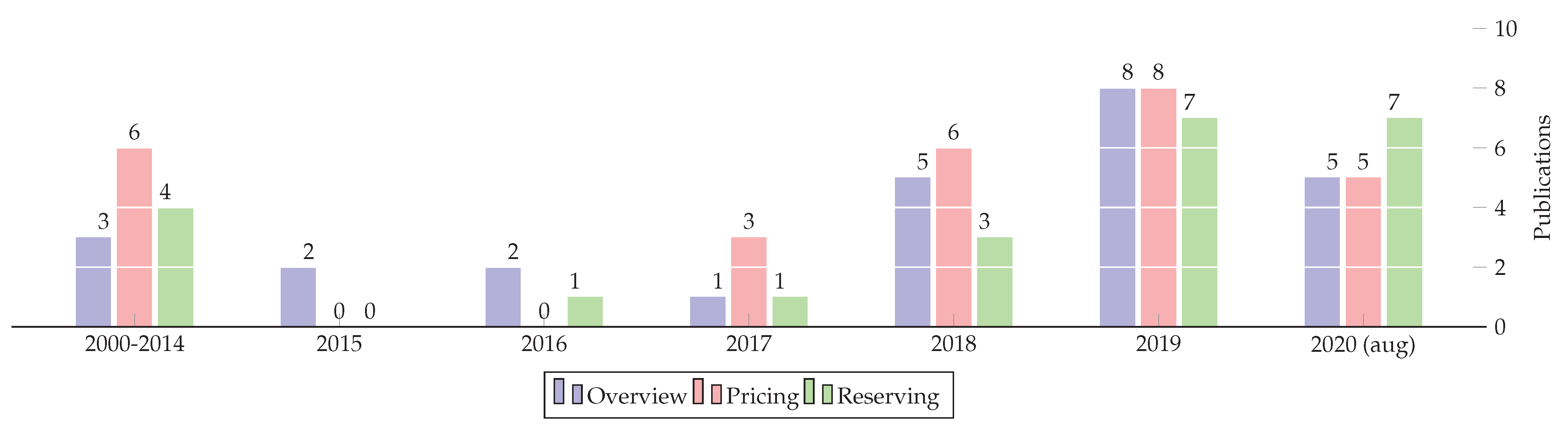
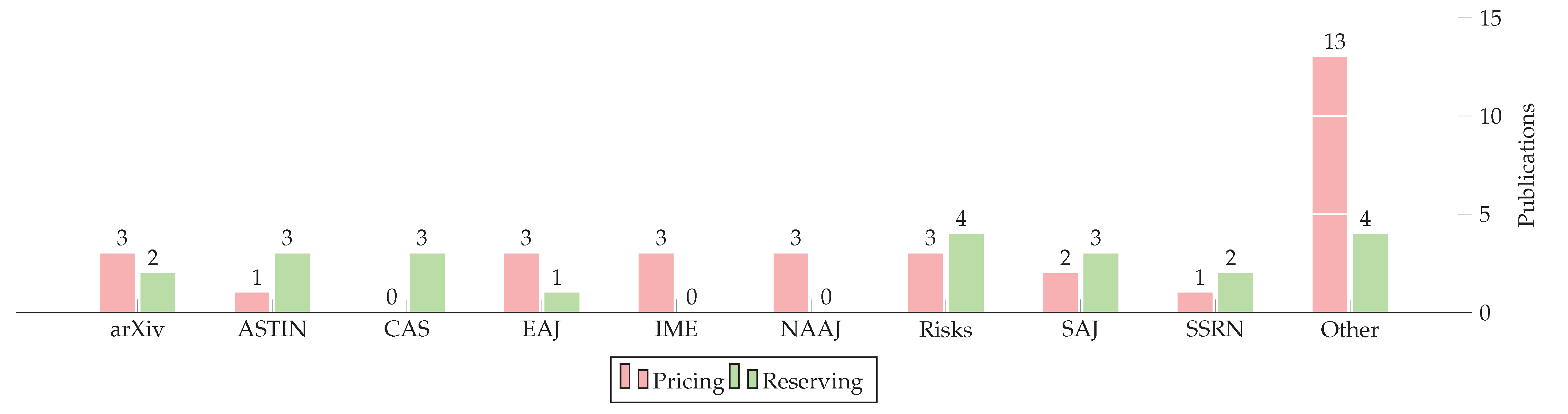
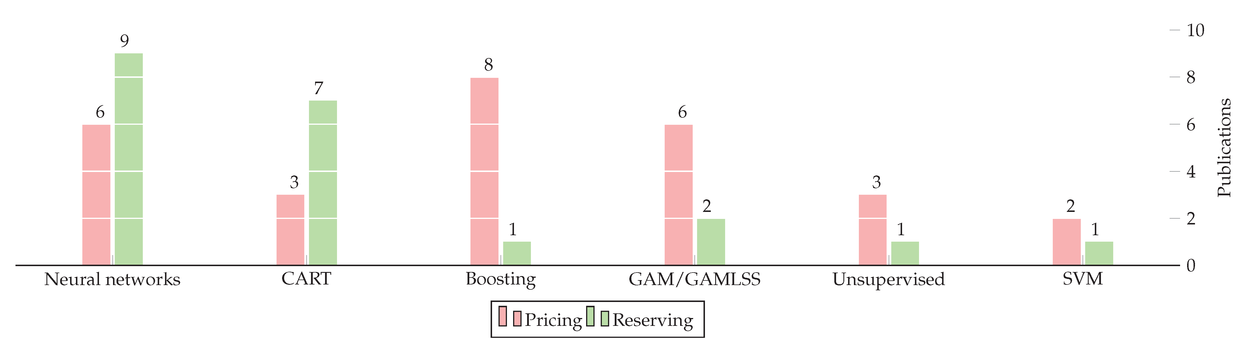
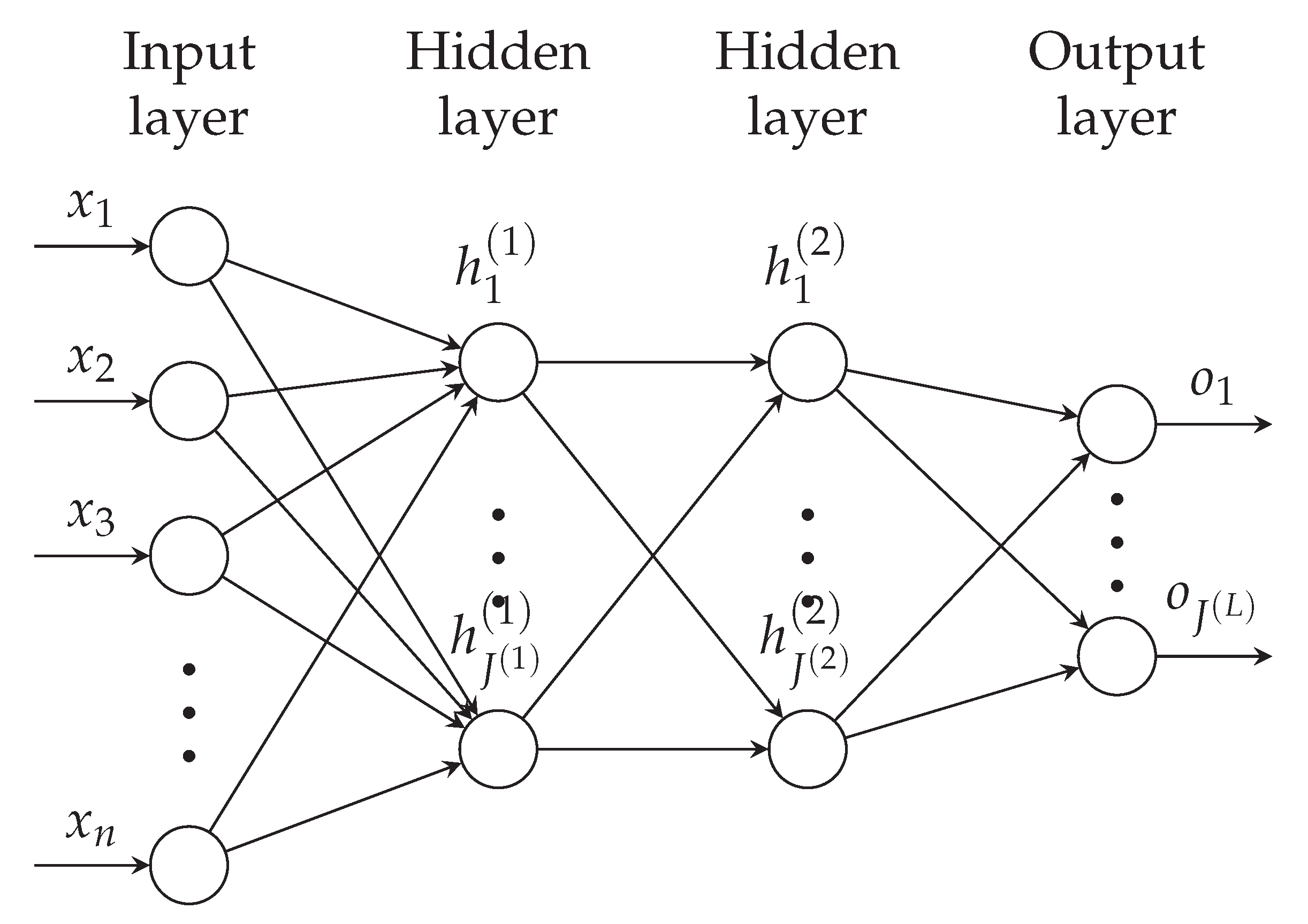
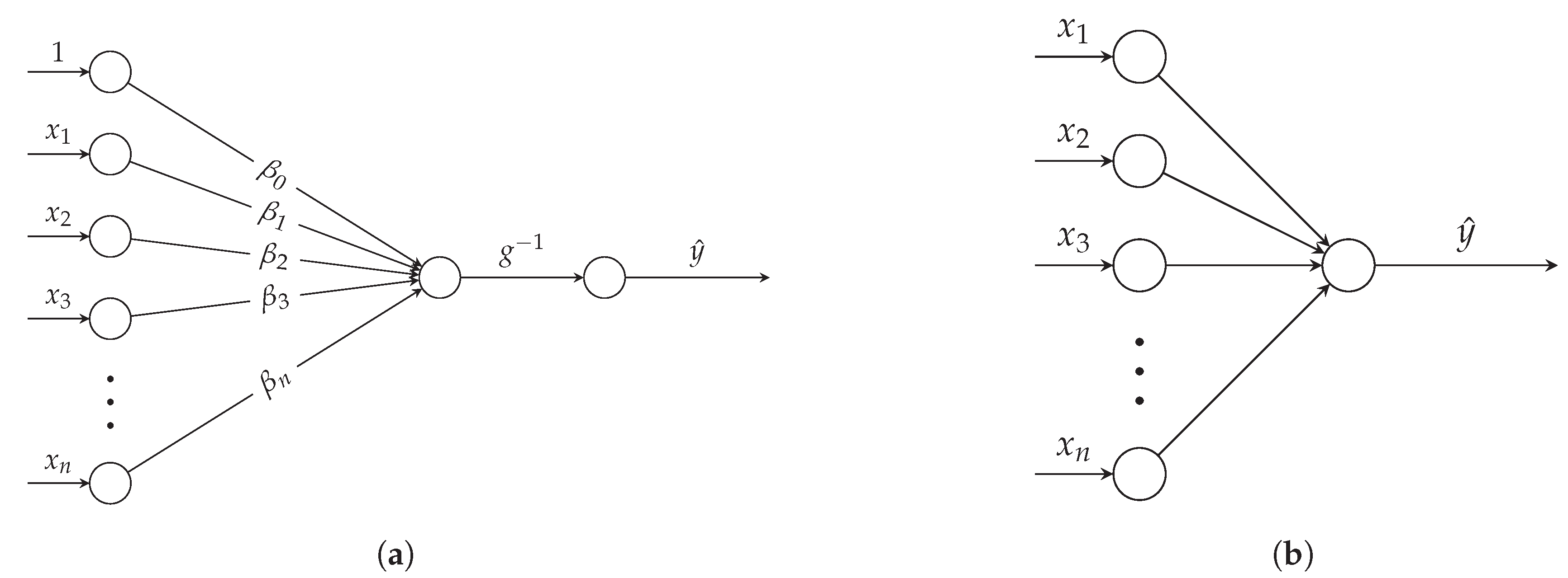
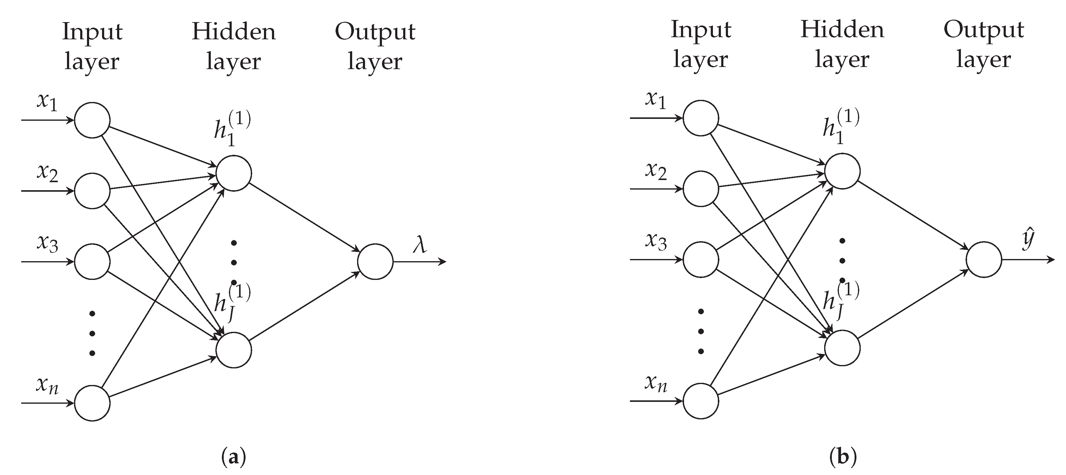
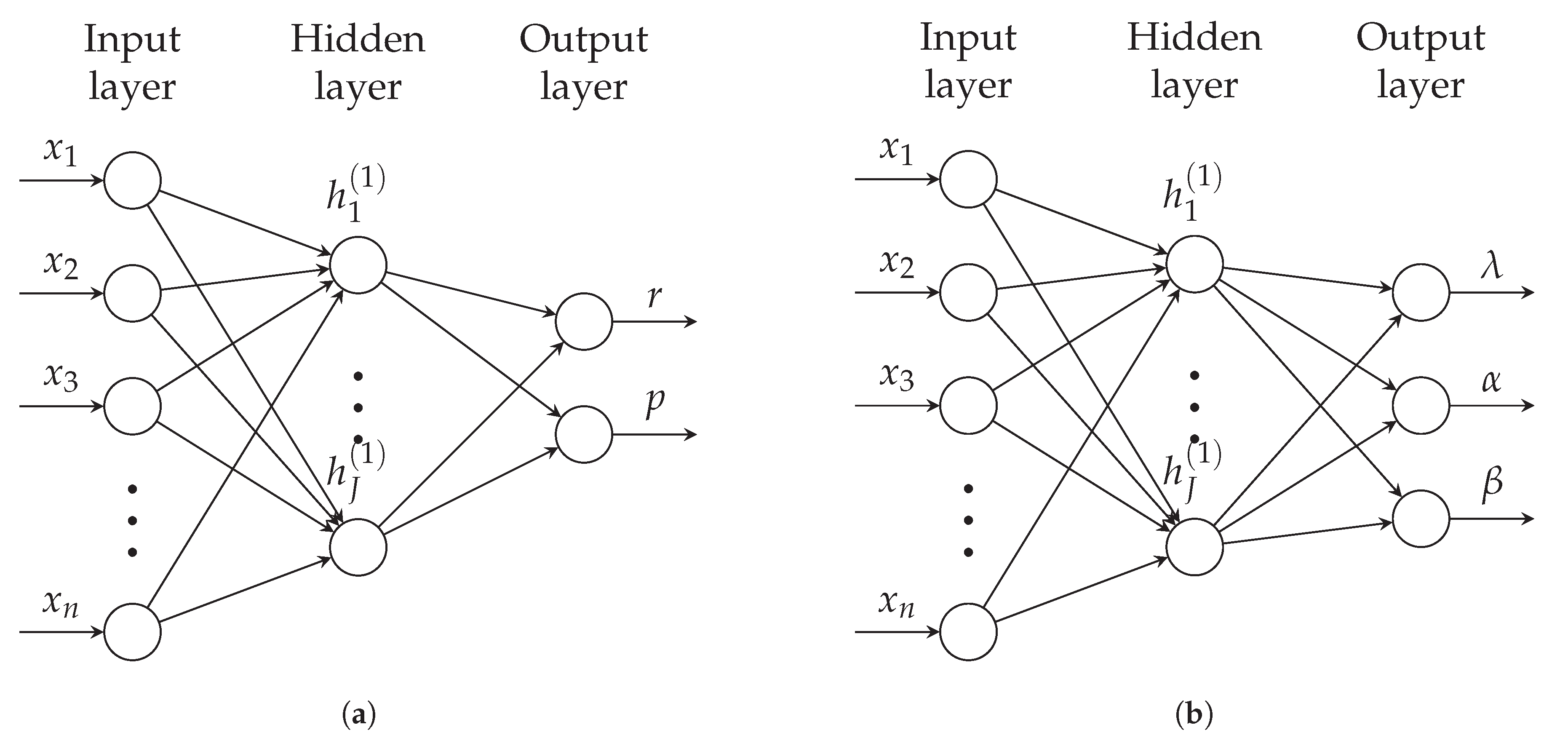
Table 1.
Overview papers on machine learning in actuarial science.
| Description | Reference | Methodologies/Approaches |
|---|---|---|
| Book | Frees et al. (2014a, 2014b) | GLM, GAM |
| Comparative study | Dugas et al. (2003) | GLM, DT, NN, SVM |
| Comparative study | Noll et al. (2018) | GLM, DT, GBT, NN |
| Comparative study | Diana et al. (2019) | GLM, RF, GBT, NN |
| Comparative study | Lee and Antonio (2015) | GLM, GAM, NN, GBT, CART |
| Comparative study | Kašćelan et al. (2016) | SVR, Kernel LR |
| Comparative study | Fauzan and Murfi (2018) | GBT, AdaBoost, RF, NN |
| Comparative study | Maynard et al. (2019) | XGBoost, RF, LR, NN, |
| Lecture notes | Wuthrich and Buser (2019) | GLM, GAM, NN, RF, GBM, SVM |
| Lecture notes | Denuit et al. (2019a, 2019b, 2019c) | GLM, GAM, GBM, NN |
| Report | Bothwell et al. (2016) | – |
| Report | Harej et al. (2017) | NN |
| Report | Jamal et al. (2018) | RF, NN, GBM |
| Review | Corlosquet-Habart and Janssen (2018) | NN, RF, GBM, SVM |
| Review | Albrecher et al. (2019) | – |
| Review | Grize et al. (2020) | CART, NN, XGBoost |
| Review | Śmietanka et al. (2020) | – |
| Review | Richman(2020a, 2020b) | NN |
| Survey | Rioux et al. (2019) | – |
| White paper | Bruer et al. (2015) | – |
| White paper | Panlilio et al. (2018) | GLM, GBT, NN |
| White paper | Richman et al. (2019) | NN |
Table 2.
Summary of contributions in pricing.
| Reference | Models |
|---|---|
| Christmann (2004) | LR, SVR |
| Denuit and Lang (2004) | GAM |
| Paglia and Phelippe-Guinvarc’h (2011) | CART |
| Guelman (2012) | GBT |
| Liu et al. (2014) | SVC |
| Klein et al. (2014) | GAMLSS |
| Sakthivel and Rajitha (2017) | NN |
| Henckaerts et al. (2018) | GAMLSS |
| Quan and Valdez (2018) | DT |
| Yang et al. (2018) | GBT |
| Lee and Lin (2018) | Boosting |
| Yang et al. (2019) | NN |
| Wüthrich and Merz (2019) | GLM, NN |
| Fontaine et al. (2019) | GLM |
| Diao and Weng (2019) | CART |
| Wüthrich (2019) | NN |
| So et al. (2020) | Adaboost |
| Zhou et al. (2020) | GBT |
| Henckaerts et al. (2020) | GBT |
Table 3.
Summary of contributions in telematics pricing.
| Reference | Models |
|---|---|
| Boucher et al. (2017) | GAM |
| Wüthrich (2017) | k-means |
| Gao and Wüthrich (2018) | PCA, AE |
| Gao et al. (2018) | GAM |
| Gao et al. (2019) | GAM |
| Pesantez-Narvaez et al. (2019) | LR, GBT |
| Gao and Wüthrich (2019) | CNN |
| Narwani et al. (2020) | LR, GBT, k-means |
| Gao et al. (2020) | CNN |
Table 4.
Summary of contributions in reserving.
| Description | Reference | Approaches | Type |
|---|---|---|---|
| ODP | England and Verrall (2001) | GAM | Agg |
| ODP | Spedicato et al. (2014) | GAMLSS | Agg |
| IBNR | Lopes et al. (2012) | SVR | Agg |
| CL | Wüthrich (2018b) | NN | Agg |
| Tot Res | Kuo (2019a) | RNN | Agg |
| ODP | Gabrielli et al. (2019) | NN | Agg |
| ODP | Gabrielli (2020b) | NN | Agg |
| — | Mulquiney (2006) | NN | Ind |
| Tot Res | Wüthrich (2018a) | CART | Ind |
| RBNS | Llaguno et al. (2017) | — | Ind |
| RBNS | Lopez et al. (2016) | CART | Ind |
| Tot Res | Baudry and Robert (2019) | CART | Ind |
| Simulation | Gabrielli and Wüthrich (2018) | NN | Ind |
| Tot Res | Pigeon and Duval (2019) | GBT | Ind |
| RBNS | Lopez et al. (2019) | CART | Ind |
| RBNS | Kuo (2020) | RNN | Ind |
| RBNS | Lopez and Milhaud (2020) | CART | Ind |
| RBNS | Gabrielli (2020a) | NN | Ind |
| RBNS | De Felice and Moriconi (2019) | CART | Ind |
| CL | Carrato and Visintin (2019) | k-means | Ind |
| Tot Res | Delong et al. (2020) | NN | Ind |
| RBNS | Crevecoeur and Antonio (2020) | GBM | Ind |
| RBNS | Lopez and Milhaud (2020) | CART | Ind |
Publisher’s Note: MDPI stays neutral with regard to jurisdictional claims in published maps and institutional affiliations. |
© 2020 by the authors. Licensee MDPI, Basel, Switzerland. This article is an open access article distributed under the terms and conditions of the Creative Commons Attribution (CC BY) license (http://creativecommons.org/licenses/by/4.0/).
Share and Cite
MDPI and ACS Style
Blier-Wong, C.; Cossette, H.; Lamontagne, L.; Marceau, E. Machine Learning in P&C Insurance: A Review for Pricing and Reserving. Risks 2021, 9, 4. https://0-doi-org.brum.beds.ac.uk/10.3390/risks9010004
AMA Style
Blier-Wong C, Cossette H, Lamontagne L, Marceau E. Machine Learning in P&C Insurance: A Review for Pricing and Reserving. Risks. 2021; 9(1):4. https://0-doi-org.brum.beds.ac.uk/10.3390/risks9010004
Chicago/Turabian StyleBlier-Wong, Christopher, Hélène Cossette, Luc Lamontagne, and Etienne Marceau. 2021. "Machine Learning in P&C Insurance: A Review for Pricing and Reserving" Risks 9, no. 1: 4. https://0-doi-org.brum.beds.ac.uk/10.3390/risks9010004
Note that from the first issue of 2016, this journal uses article numbers instead of page numbers. See further details here.