Alleviating Class Imbalance in Actuarial Applications Using Generative Adversarial Networks


1
School of Computer Science and Applied Mathematics, University of the Witwatersrand, West Campus, Mathematical Sciences Building, Private Bag 3, Wits, Braamfontein 2050, South Africa
2
DSI-NICIS National e-Science Postgraduate Teaching and Training Platform (NEPTTP), Wits, Braamfontein 2050, South Africa
3
School of Statistics and Actuarial Science, University of the Witwatersrand, West Campus, Mathematical Sciences Building, Private Bag 3, Wits, Braamfontein 2050, South Africa
*
Author to whom correspondence should be addressed.
Risks 2021, 9(3), 49; https://0-doi-org.brum.beds.ac.uk/10.3390/risks9030049
Submission received: 19 October 2020
/
Revised: 11 November 2020
/
Accepted: 21 November 2020
/
Published: 8 March 2021
(This article belongs to the Special Issue Data Mining in Actuarial Science: Theory and Applications)
Abstract
:To build adequate predictive models, a substantial amount of data is desirable. However, when expanding to new or unexplored territories, this required level of information is rarely always available. To build such models, actuaries often have to: procure data from local providers, use limited unsuitable industry and public research, or rely on extrapolations from other better-known markets. Another common pathology when applying machine learning techniques in actuarial domains is the prevalence of imbalanced classes where risk events of interest, such as mortality and fraud, are under-represented in data. In this work, we show how an implicit model using the Generative Adversarial Network (GAN) can alleviate these problems through the generation of adequate quality data from very limited or highly imbalanced samples. We provide an introduction to GANs and how they are used to synthesize data that accurately enhance the data resolution of very infrequent events and improve model robustness. Overall, we show a significant superiority of GANs for boosting predictive models when compared to competing approaches on benchmark data sets. This work offers numerous of contributions to actuaries with applications to inter alia new sample creation, data augmentation, boosting predictive models, anomaly detection, and missing data imputation.
1. Introduction
1.1. Background
Gaining an advantage in competitive markets through offerings of suitable tailored products on customers relies on building and maintaining adequate predictive models. To build these models, a substantial amount of data and a sizeable number of records is desirable. However, when expanding to new or unexplored markets, that level of information is rarely always available. To build such models, actuarial firms often have to procure data from local providers, use limited unsuitable industry and public research or rely from extrapolations from other better known markets.
In this work, we show how an implicit model using the Generative Adversarial Network (GAN) Goodfellow et al. (2014) can alleviate this problem through the generation of adequate quality data even from very limited small samples, from difficult domains, or without alignment, thus handling class imbalance.
A GAN is an example of a generative model that is used to create new samples from a latent noise space. A generative model describes how a data set is generated in terms of a probabilistic model. This generative model mimics the training data distribution as close as possible. If this is achieved, then we can sample from to generate realistic samples that appear to have been drawn from . We are satisfied if our model can also generate diverse samples that are suitable different from the training data. In some cases, the model can be estimated explicitly, and sometimes it can generate samples implicitly. Other models are capable of doing both.
GANs were proposed in a seminal paper by Goodfellow et al. (2014). GANs are useful for learning the structure of the data and can generate new samples without explicitly postulating the model Goodfellow et al. (2014). They are known to be better than other generative models due to the quality of samples they generate. GANs have been highly successful in computer vision Brock et al. (2018); Karras et al. (2019); Zhu et al. (2017); Vondrick et al. (2016), music generation Yang et al. (2017), text generation Reed et al. (2016), missing data imputation Li et al. (2019); Shang et al. (2017); Yoon et al. (2018), time series generation Esteban et al. (2017); Yoon et al. (2019); Fu et al. (2019), and data augmentation Antoniou et al. (2017); Fiore et al. (2019); Mariani et al. (2018); Mottini et al. (2018); Park et al. (2018), with remarkable results, but their application to the actuarial discipline remains largely still unexplored.
In this work, we discuss how and where GANs can be used by actuaries. Additionally, we provide an experiment showing how GANs can be used to boost imbalanced samples in actuarial data sets and improve actuarial models.
1.2. Aims and Objectives
In this paper, we explain what GANs are and how they can be used to synthesize data in order to accurately enhance very infrequent events, alleviate class imbalance and create better prediction models. This work also provides theoretical and practical applications of GANs.
We demonstrate a popular GAN architecture to a typical problem resembling an actuarial use on benchmark data sets using Python Python Software Foundation (2017). Overall, we show a significant superiority of GANs for predictive models and stochastic simulations compared to current approaches. Specifically, this paper covers the following aims and objectives:
- deep overview of generative models and why GANs are of better quality than other generative models;
- an overview of GANs with practical applications in a number of areas with emphasis for actuarial use; and
- provide a practical example of a popular GAN use for alleviating class imbalance, data augmentation, and improving predictive models.
1.3. Contribution
This work provides thorough theoretical, empirical and practical applications of GANs, with possible leverage in actuarial science for inter alia new sample creation, data augmentation, boosting actuarial models, anomaly detection, missing data imputation, time series simulations and projections in life insurance, short-term insurance, health and care, banking, investment, enterprise risk management, and other non-traditional actuarial areas, such as telecommunications, economics, medicine, engineering, and other wider fields.
For example, actuaries build pricing models in order to determine competitive premiums that customers should pay to be provided adequate insurance coverage O’Malley et al. (2005). These pricing models are dependant on risk events, such as mortality, morbidity, and lapse, which need to be estimated using an adequate and accurate model. However, these risk events are often under-represented in data.
In this work, we show how a GAN could be used to alleviate this problem through the generation of adequate quality data from limited or highly imbalanced samples. Essentially, we show that synthetic data generated using GANs can augment imbalanced data sets, leading to significantly higher predictive power of possible actuarial models fitted after.
1.4. Structure of the Paper
The rest of the paper is organized as follows. Section 2 describes the problem of class imbalance and its common solutions. Section 3 reviews the literature on generative models, with particular emphasis on GANs, while Section 4 covers GAN applications, especially for actuarial adoption. Section 5 describes the methodology followed. Section 6 outlines the example experiments conducted. Section 7 presents the results, and Section 8 discusses the results, while Section 9 gives conclusions, limitations, and possible future work.
2. Class Imbalance
2.1. Definition
Whilst machine learning (ML) has gained significant prevalence in the past few decades, class imbalance, limited data sets, and missing data remain pervasive problems Chawla et al. (2002); Fernández et al. (2018); Longadge and Dongre (2013). These issues occur due to the nature of the data space, data collection costs, data limitations, new markets, and absolute rarity.
In binary classification problems, class imbalance occurs when one of the classes has overwhelmingly more instances than others. ML classifiers tend to have skewed accuracy towards the majority class when the data is imbalanced Chawla (2009); Fernández et al. (2018). This is problematic as misclassifying a minority class can result in significant misclassification costs than for the majority case Chawla et al. (2002). Class imbalance arises because ML classifiers do not necessarily take into account unequal class distributions. This problem causes a significant and an unexpected performance behavior for most classifiers.
2.2. Techniques to Alleviate Class Imbalance
Techniques as shown in Figure 1 exist to alleviate class imbalance, and these techniques include re-sampling, algorithmic-level solutions, cost-sensitive learning, ensembles, and generative models.
2.2.1. Re-Sampling
Re-sampling techniques modify the training data such that the distribution of the classes is evenly balanced where the majority or minority class is either under-sampled or over-sampled. Over-sampling has been the most frequently used technique than under-sampling since under-sampling eliminates important information in the majority class.
Hybrid sampling techniques combine over-sampling with data cleaning techniques, informed under-sampling techniques, or greedy-filtering approaches Batista et al. (2004), thereby eliminating redundant and noisy instances, boosting the predictive accuracy of models trained after.
2.2.2. Synthetic Sampling
A pioneering and popular method to alleviate class imbalance has been Synthetic Minority Over-sampling TEchnique (SMOTE) Chawla et al. (2002). However, SMOTE suffers from over-fitting, over-lapping classes, noisy examples, is less reliant on the true probability distribution, and alters the original distribution of the minority classes, and this may not be desirable Batista et al. (2004); Ganganwar (2012); Longadge and Dongre (2013).
There have been few empirical reviews which compare and synthesize SMOTE and its density-based variants Gao et al. (2014). There have been few approaches which create synthetic samples by sampling implicitly from the minority class distribution. Current density-based approaches may be subjective as they need to pre-specify the format and structure of the minority class distribution Das et al. (2015); Zhang and Li (2014). Generative models offer a significant alternative, yet these models have not been thoroughly explored in imbalanced learning. In this work, we show how a popular implicit generative model can be used to handle class imbalance and rival SMOTE.
2.2.3. Ensembles
Ensemble is where a classifier’s accuracy is increased by the use of training on different over-sampled data sets or different algorithms and combining outputs to a single outcome. These approaches tend to improve the results of re-sampling techniques Chawla et al. (2003); Wang and Yao (2009). However, they can take a long time to compute and still do not solve the true data distribution issue.
2.2.4. Other Methods
Algorithmic-level solutions modify the ML classifier to adjust for the presence of class imbalance in the data. Cost-sensitive learning incorporates mis-classification costs in the evaluation metric Ganganwar (2012). This approach is more computationally efficient than data-level solutions He and Garcia (2008). However, mis-classification costs are often unknown and difficult to set, making this method less popular than sampling techniques López et al. (2013).
SMOTE and its variants remain the most studied and widely used solutions, with generative models slowly being adopted in alleviating class imbalance Fernández et al. (2018); Fiore et al. (2019); Gao et al. (2014). Generative models are described in detail in Section 3.
3. Generative Models
This research is concerned with handling class imbalance through generative modeling. Other approaches exist, such as synthetic sampling; however, these approaches do not take into account the underlying structure of the data distribution and often lead to over-fitting and over-lapping cases Gao et al. (2014). Generative models are flexible models capable of learning the data distribution and sampling from this data distribution, thereby creating new synthetic cases. In this section, we review generative models and explain why GANs are of better quality than other deep generative models.
3.1. Definition
Given a data set with observations X, we assume that X has been generated from an unknown true probability distribution . A generative model mimics as close as possible. If this is achieved, then we can sample from to generate realistic samples that appear to have been drawn from .
We are satisfied if our model can also generate diverse samples that are suitable different from X. In some cases, the model can be estimated explicitly and sometimes it can generate samples implicitly. Other models are capable of doing both. GANs provide no estimate of the model but are capable of generating new data without knowing it.
Goodfellow (2016) provides a taxonomy of common deep generative models shown in Table 1, divided into implicit and explicit models. GANs are designed to remedy most of the disadvantages that come with explicit models and other Markov chain models.
3.2. Explicit Models
Explicit models specify or approximate a parameterized log-likelihood representation of the data Goodfellow et al. (2014). Parameters are then estimated and learned from the data and this requires a maximum likelihood estimation which integrates over the entire data space, and this may be intractable Li et al. (2015). These approximation techniques may not always yield the best results as some of them rely on Markov chains, which are time-consuming Goodfellow et al. (2014).
Two popular tractable models are fully visible belief networks (FVBNs) Frey et al. (1996) and nonlinear independent component analysis (ICA). Approximate methods improve on the design of tractable models which can be computational intensive and limited Goodfellow et al. (2014); Makhzani et al. (2015); Rezende et al. (2014). Approximate methods use either deterministic, i.e., variational inference, or stochastic approximations such as Markov chain Monte Carlo (MCMC) Geyer (1992). Variational inference involves the use of Variational Autoencoders (VAEs) Kingma and Welling (2013); Rezende et al. (2014) to approximate using lower bounds.
3.2.1. FVBNs
FVBN estimates the probability density of the training data into a decomposed product of one-dimensional probability distributions. This model outputs a probability for each possible value if x is discrete and outputs a network of parameters of a simple distribution if x is continuous. Using the generated model, sampling is done one step at a time, conditioned on all previous steps Goodfellow et al. (2014).
The problem with these models is their computational complexities as they need to generate one point at a time. Other problems include poor learning representations, over-emphasizing details over global data, and not closely reflecting the true generation process Goodfellow (2016). Moreover, these models have been more useful for image synthesis than structured data sets, such as tabular data Van den Oord et al. (2016). GANs are known to provide new samples in parallel, thus yielding greater speed of generation Goodfellow (2016); Li et al. (2015).
3.2.2. Non-Linear ICA
Non-linear ICA involves defining some continuous non-linear transformations of data between high dimensions and lower dimensional spaces. The distribution of the data is transformed into a distribution of a latent space z defined by , where g is some tractable transformed version of . The challenge in ICA is finding tractable distributions in the latent space, and these are limited Goodfellow et al. (2016). GANs are known to have fewer restrictions than these models Goodfellow et al. (2014); Bengio et al. (2014); Goodfellow (2016).
3.2.3. Variational Autoencoders
VAEs, along with FVBNs and GANs, are three of the most popular approaches for sample generation. VAEs are an extension to AEs Bellinger et al. (2016); Larsen et al. (2015); Rezende et al. (2014). AE learns useful representations of the data by encoding X into a compressed latent space z using and then decoding z back into X using by minimizing the reconstruction error between the original data and the deconstructed data Bellinger et al. (2016). VAE maximizes the following function:
Unlike auto-regressive models, VAEs are normally easy to run in parallel during training and inference Goodfellow et al. (2016); Larsen et al. (2015); Rezende et al. (2014). Conversely, they are normally harder to optimize than auto-regressive models Goodfellow et al. (2016); Makhzani et al. (2015). The encoder converts the input to latent space representations through the mean and variance, and samples can be created from the learned representation. VAEs have been criticized to be generating blurry samples and are intractable Goodfellow et al. (2016); Salimans et al. (2016).
3.2.4. Boltzmann Machines
Boltzmann machines rely on the use of Markov chains to model and to sample from it Ackley et al. (1985); Hinton (2002); Salakhutdinov and Hinton (2009). A Markov chain is a process that is used to generate samples by repeatedly drawing a sample from a transition operator Geyer (1992). A Boltzmann machine is an energy-based function defined as:
where is an energy function, and Z is a normalizing factor to ensure that sums to one Ackley et al. (1985); Goodfellow et al. (2016).
These methods include restricted boltzmann machine (RBM) Ackley et al. (1985) and deep belief networks (DBNs) Hinton et al. (2006); Hinton and Salakhutdinov (2006). DBNs and RBMs are generative stochastic neural networks that can estimate a probability distribution Ackley et al. (1985). Samples are obtained through MCMC runs to convergence, and this can be very expensive to run Li et al. (2015). These models were pioneers in early 2006 for deep generative models, but they have been rarely used because of poor scale-ability for higher dimension problems and high computational costs Goodfellow et al. (2016).
3.3. Implicit Models
Implicit models learn to model the true distribution and define a stochastic procedure to directly generate new data from a latent space. These models can be trained indirectly without needing an explicit density function to be learned or defined. Some of these models, such as the Generative Stochastic Network (GSN) Bengio et al. (2014), involve MCMC methods, which impose greater computational cost and often fail to scale to higher dimensional spaces Goodfellow et al. (2016). GANs Goodfellow et al. (2014) and Generative Moment Matching Networks (GMMNs) Li et al. (2015) are one of the few implicit probabilistic models capable of sampling in parallel and in a single step.
GANs were designed to remedy most of the issues with explicit and some implicit models. GANs are known to parallelize sample generation, have fewer restrictions, subjectively thought to produce better samples, make no use of Markov chain or maximum likelihood estimation, and assume no variational bounds and no distributional assumptions Arjovsky et al. (2017); Goodfellow et al. (2016). As a result, GANs have generated a lot of interest since 2014, with wide applications in many areas.
3.3.1. GANs
GANs were originally invented in a landmark paper by Ian Goodfellow in 2014 Goodfellow et al. (2014). The setup of the framework uses an adversarial process to estimate the parameters of two artificial neural network (ANN) Rumelhart et al. (1986) models by iteratively and concomitantly training a discriminator (D) and a generator (G), as shown in Figure 2.
Through multiple cycles of generation and discrimination, both networks train each other, while simultaneously trying to outwit each other Goodfellow et al. (2014); Mariani et al. (2018); Odena et al. (2017); Zhu et al. (2017). GANs have two adversarial ANNs:
- G picks z from the prior latent space Z and then generates samples from this distribution using ANN;
- D receives generated samples from G and the true data examples, and it must distinguish between the two for authenticity.
Both D and G are ANNs which play a zero-sum game, where G learns to produce realistic-looking samples and D learns to get better at discriminating between the generated samples and the true data. Once G is trained to optimality, it can create new samples and augment the training data set. GANs can sample in parallel better than other generative models, have fewer restrictions on the generator function, assume no use of Markov Chains, as well as no variational bounds, unlike VAE, and produce subjectively better quality samples than other generative models Arjovsky et al. (2017); Goodfellow et al. (2016); Goodfellow et al. (2014); Radford et al. (2015); Salimans et al. (2016).
Whilst GANs are gaining popularity in many applications, they have notable issues. GANs are notoriously difficult to train properly and difficult to evaluate, the likelihood cannot be easily be computed, and they suffer from the vanishing gradient problem, mode collapse, boundary distortion, and over-fitting Arjovsky et al. (2017); Goodfellow et al. (2016); Salimans et al. (2016).
Mode collapse is when many latent noise values z are mapped to the same data point x, leading to a lack of diversity in the samples that are created, i.e., under-fitting. The vanishing gradient problem occurs when D becomes perfect in its training without giving G the chance to improve. As a result, GANs may fail to converge, thereby leading to poor generated samples Arjovsky et al. (2017). Figure 3 provides a non-exhaustive taxonomy of GAN variants and improved training, including common examples Creswell et al. (2018); Hitawala (2018); Hong et al. (2019); Wang et al. (2017).
For GAN reviews, (Creswell et al. (2018); Hitawala (2018); Hong et al. (2019)) provide a comparative overview. Lucic et al. (2018) conduct an in-depth study on GANs and note no significant performance differences on the GANs studied. There are over 300 GAN variants, and it is impossible to review all of them. In this work, we are interested in exploring GAN applications and showing their potential to actuaries, especially for alleviating class imbalance, data augmentation, and improving the predictive ability of actuarial models.
3.3.2. GMMNs
GMMNs minimize the maximum mean discrepancy (MMD) between the moments of and and are known to be simpler than other generative models Li et al. (2015). Moment matching evaluates whether the moments of the true distribution match those of the data through MMD. This approach is similar to GANs in terms of training, except using a different loss function, which leads to faster sampling. However, GMMNs have received less attention than GANs and VAEs, limiting their sample generative scheme Arjovsky et al. (2017); Goodfellow et al. (2016); Hitawala (2018).
3.4. Summary
There are a number of deep generative models for synthetic sample generation. Some of the models are explicit with an intractable likelihood and inference. Some models are only approximate and generate blurry samples. Other methods do not sample in parallel, are complex, and rely on Markov chains, which are time-consuming. GANs are attractive as they do not make any explicit density estimation, and they remedy most of these issues. GANs have generated extremely good examples in many domains. Section 4 reviews these GAN applications.
4. Applications of GANs
The most successful applications of GANs are in computer vision, but there have been applications in other domains, as well. In this section, we focus on the applications where there is some actuarial use.
4.1. Data Augmentation
The availability of sufficient data in many domains is a necessity, especially where predictive models are needed to make business decisions. Such models are built on adequate training data for better generalization and meaningful accuracy Goodfellow et al. (2016). In this work, we are interested in adopting GANs for new sample creation and data augmentation in order to boost predictive models by supplementing training data sets with new samples that are learned from the real data distribution in an adversarial manner. Data augmentation is a procedure to create synthetic cases to augment the training data and increase its size, especially for those data points that are lacking. This is where GAN shines—the ability to create new samples and adequate data sets Goodfellow et al. (2014); Fiore et al. (2019).
There are two main strategies to check if this augmentation really helped something: we can train our model on fake data and check how well it performs on real samples. We can also train our model on real data to do some classification task and only after check how well it performs on generated data. If it works well in both cases—you can feel free to add samples from the generative model to your real data and retrain it again—you should expect gain of performance.
Recently, a number of papers have applied GANs to augment various data sets, with remarkable results on the performance of the predictive models applied after Antoniou et al. (2017); Douzas and Bacao (2018); Fiore et al. (2019); Mariani et al. (2018); Mottini et al. (2018); Park et al. (2018); Xu et al. (2019); Ding et al. (2019). Similarly, GANs can be used to augment actuarial data sets and boost actuarial models, making them more accurate and less biased. In this work, we demonstrate how this can be done for a number of data sets, described in Section 6.
4.2. Anomaly Detection
Anomaly detection is the identification of rare items, events, or observations which raise suspicions by differing significantly from the majority of the data. Anomaly detection finds extensive use in a wide variety of applications, such as fraud detection for credit cards, insurance, or health care. The importance of anomaly detection is due to the fact that anomalies in data translate to significant (and often critical) actionable information in a wide variety of application domains. There are a number of these methods, such as clustering-based, classification-task, nearest neighbor, spectral, or statistical, but most of them have rather strong assumptions and long training times.
Main generative models, like VAE or GAN, consist of two parts. VAE has an encoder and the decoder, where the encoder basically models the distribution and the decoder reconstructs from it Larsen et al. (2015). A GAN consists of the generator and the discriminator, where the generator models the distribution and the discriminator judges if it is close to the training data Goodfellow et al. (2014). They are pretty similar in some way—there is modeling and judging part (in VAE, we can consider reconstructing as some kind of judgement).
The modeling part is supposed to learn the data distribution. What will happen to the judging part if we give it some sample not from the training distribution? In case of a well trained GAN, the discriminator will tell us 0, and reconstruction error of VAE will be higher than average one on the training data Akcay et al. (2018). Our unsupervised anomaly detector is then easily trained and evaluated. We can feed it with some steroids, like statistical distances, if we want.
In medicine, Schlegl et al. (2017) propose an AnoGAN for anomaly detection of medical images, and learn the characteristics of lesions by learning the characteristics of health data sets. Akcay et al. (2018) present GANomaly for anomaly detection in visual noise, noting a significant improvement on detecting anomalies on various data sets. These methods can be leveraged for potential applications in fraud detection, lapse prediction and claiming likelihood in insurance. A GAN useful and leveraged for anomaly detection can rival other anomaly detection techniques.
4.3. Time Series
Suppose we wanted to simulate the evolution of a stock price for some particular asset using traditional simulations, such as Monte Carlo. We would need to estimate the mean and volatility of the returns using past price evolution and then simulate new prices under the assumption that the returns follow a Gaussian distribution with the estimated parameters. However, this normality assumption may not be entirely true in practice where there is a tendency for higher observed probabilities for the tail events than those predicted by the Gaussian distribution. We could change our assumption, say, into a student-t distribution, but neither would that assumption completely describe the reality. GANs are capable of replicating the price evolution without making any model assumptions.
Time series and stochastic processes are widely used by financial firms for risk management, financial projections, stock prediction, extreme event monitoring, and monetary policy making Fu et al. (2019). Traditionally, autoregressive time series models, exponential smoothing and their variants, and, more recently, deep learning, have been introduced and intensively studied and applied for time series data Esteban et al. (2017).
However, most of these models rely on strong dependence on model assumptions and model parameter estimation and, thus, are less effective in the estimation of complex distributions with time-varying features Zhou et al. (2018). GANs do not make any explicit assumptions and are capable of learning the distributions and their dependence structures in a non-parametric fashion. There has been a number of time series GANs proposed, such as the recurrent conditional GAN (RCGAN) Esteban et al. (2017) and time series GAN (TimeGAN) Yoon et al. (2019), for the generation of realistic financial time series.
Immediate actuarial uses leveraging these GANs are stochastic simulations, capital modeling, mortality projections, reserving, asset and liability management, solvency projection, and other time series generation tasks. GANs can be used to rival Monte Carlo or stochastic simulations without any distributional assumptions. In insurance, mortality forecasting is an important actuarial task. Typically, mortality forecasting models, such as Lee-Carter Lee and Carter (1992), are used, but these make strong mathematical assumptions which need to be validated by the data. Time series GANs could potentially be used to simulate and project mortality rates into the future, potentially competing with existing models.
4.4. Privacy Preservation
Data of a lot of companies can be secretive, confidential, or sensitive. Sometimes, we need to share it with third parties like consultants or researchers. If we want to share a general idea about our data that includes the most important patterns, details, and shapes of the objects, we can use GANs directly to sample examples of our data to share with other people without sharing identifiable features. This way we will not share any exact confidential data, just something that looks exactly like it.
Privacy-preservation GANs are capable of accomplishing this task Beaulieu-Jones et al. (2019). In actuarial valuation models where model points are used to determine the amount of money to hold for an individual/groups, such GANs may be useful for the creation of synthetic samples to be fed into the valuation model, without needing the details of any policy. In particular, GANs can be used to share synthesized data and make them publicly available, increasing the scope for actuarial research, collaboration, and comparisons.
4.5. Missing Data Imputation
Missing data causes an issue in analysis as most standard data analytic methods are not designed for missing data. Techniques, such as single imputation (SI) and multiple imputation (MI) Rubin (2004), exist, but there is no consensus on which of the MI method is superior, even though MI is known to be better than SI Schafer and Olsen (1998).
Generative Adversarial Imputation Net (GAIN) Yoon et al. (2018) provides an alternative generative modeling approach to create new cases that can be used to impute missing information. View Imputation via GANs (VIGAN) Shang et al. (2017) deals with data that are collected from heterogeneous sources, resulting in multi-view or multi-modal data sets where missing data occurs in a number of these sources. These methods were shown to be better than SI/MI methods, thereby improving the effectiveness of ML algorithms trained after. These GANs can be used to impute missing data points in experience investigations and assumption setting in both short-term and life insurance when conducting valuation or pricing, increasing the number of data points available for boosting the predictive power of models built after.
4.6. Semi-Supervised Learning
The purpose of a Semi-Supervised GAN (SGAN) is to train the discriminator into a classifier which can achieve superior classification accuracy from as few labeled examples as possible Sricharan et al. (2017), thereby reducing the dependency of classification tasks on enormous labeled data sets. It has been shown that an SGAN generalizes from a small number of training examples much better than a comparable, fully-supervised classifier Chongxuan et al. (2017); Liu et al. (2019); Miyato et al. (2018). This has been lauded as the most useful GAN application with good performance with a small number of labels on data sets Odena (2016); Salimans et al. (2016).
For imbalanced data sets, such as mortality, morbidity, fraud, lapses, extreme events, large claims, and sub-standard risks, SGAN may offer a superior alternative predictive model compared to ML models which require significant training data for improved accuracy. Typically, one has to deal with imbalanced classes either through synthetic sample generation using some heuristic method, such as SMOTE, cost sensitive adjustment to the evaluation metric, or adding uncertainty margins, which can be subjective. Through the training of an SGAN, it is possible to have a sample generative scheme whilst having a classifier, as well. This has tremendous advantages over many generative and ML models.
4.7. Domain Adaptation
It is quite possible that the training data used to learn a classifier has a different distribution from the data which is used for testing. This results in degradation of the classifier performance and highlights the problem known as domain adaptation Hong et al. (2018). In domain adaptation, the training and test data are from similar but different distributions. This area has become interesting for GANs in the past few years.
These methods include CycleGAN Zhu et al. (2017), Discover GAN (DiscoGAN) Kim et al. (2017), DualGAN Yi et al. (2017), and StarGAN Choi et al. (2018), which can be used for multiple domains. With these methods, one can transfer an algorithm learned from a different data set to a new one and achieve similar performance. Such approaches are also able to learn representation adaptation, which is learning feature representations that a discriminator cannot differentiate which domain they belong to Tzeng et al. (2017). By using synthetic data and domain adaptation, the number of real-world examples that are needed to achieve a given level of performance is reduced significantly, utilizing only randomly generated simulated points Hoffman et al. (2017). Domain adaptation can learn transfers between different domains, by synthesizing different data sets. This can be useful in combing public data sets or other market data with internal company data in actuarial firms.
4.8. Summary
Given the above taxonomy of GAN applications, Table 2 depicts specific actuarial areas where GANs can be useful.
To our knowledge, there has been limited applications of GANs in actuarial areas, such as insurance, health care, banking, investment, and enterprise risk management. This is compounded by the fact that GANs have been highly successful on computer vision, with less emphasis on tabular data sets. However, there have been recent applications of GANs on other tabular data sets, such as airline passengers Mottini et al. (2018) and medical records Armanious et al. (2018).
GANs can equally be adopted or leveraged for similar tasks to boost limited actuarial data sets and improve actuarial models, especially in areas where models are needed to make business decisions. Examples of actuarial applications with limited data and the class imbalance problem include claim frequency modeling, claim amount estimation, lapse prediction, fraud detection, mortality/morbidity rate estimation, catastrophe modeling, extreme event models, and risk estimation. Leveraging GANs to increase the data size on these data sets could lead to better actuarial models. In particular, GANs could allow less reliance on using stochastic simulations that are based on subjective distributions and err less on margins used.
5. Methodology
This section describes in detail the theoretical operation of GANs, their challenges, and tricks to improve their training. Throughout this paper, it is assumed that both GAN networks are implemented with ANNs. For comparative purposes, we also implement a popular synthetic data generative mechanism using Synthetic Minority Over-sampling Technique (SMOTE) Chawla et al. (2002).
5.1. SMOTE
This section describes the theoretical operation of SMOTE for comparative purposes with the GAN applied in this work. SMOTE creates new synthetic cases by linearly interpolating between two nearest neighbor (NN) instances of the minority class. Chawla et al. (2002) show that SMOTE improves the effectiveness of ML classifiers compared to random over-sampling and under-sampling approaches. Over time, SMOTE has become the default method for synthetic sample generation and has proven to be popular among researchers, becoming a pioneer in imbalanced learning Fernández et al. (2018).
Considering a random minority instance x, a new instance s is generated by considering its k-NNs. These k-NNs are found by using the Euclidean distance metric. Initially, an instance y is generated at random from the k-NNs. Then, a new synthetic minority instance s is generated, as follows:
where is randomly generated from the Uniform distribution .
SMOTE parameters are the value of k and the number of minority cases to generate. These parameters can be tuned to ensure an optimal metric is achieved. SMOTE is the benchmark method for addressing class imbalance in binary classification problems.
5.2. Vanilla GAN
This section describes the original GAN formulation, called MiniMax GAN (MM-GAN). This is the baseline model over which all other GAN variants are based.
5.2.1. The Discriminator
The discriminator (D) receives generated samples from a generator G and the true data examples from , and must distinguish between the two for authenticity through a deep ANN Goodfellow et al. (2014). The resulting output for an input x is the probability of x being sampled from instead of , where is the implicit distribution defined by G. The vector represents learned parameters from D. The discriminator’s goal is to yield near 1 for and closer to 0 for using the sigmoid function in the output layer. This is achieved by maximizing D’s loss over :
5.2.2. The Generator
The generator (G) randomly picks a sample z from the prior latent space defined by and then generates samples from this distribution using an ANN. This deep ANN must learn the parameters given an input , that will give the output . G is trained to fool D, i.e., to make D’s output for fake/generated sample closer to 1. The parameters of G are learned by minimizing G’ loss over :
5.2.3. GAN Loss
Combining the losses for D and G, GANs solve the following minimax game in alternate steps through Gradient Descent (GD) Ruder (2016):
The above losses for D and G are the original formulation proposed by Goodfellow in 2014, called minimax GAN (MM-GAN). Since we are minimizing over and maximizing over , training of GANs alternate between GD on G and gradient ascent on D Goodfellow et al. (2016). Typically, for every training of G, D is trained k times although an optimal choice is debatable among researchers. This is shown in Algorithm 1.
Remark 1.
Gradient based updates on the networks can be accomplished using one of the GD optimizers. Typically, Stochastic GD (SGD) with Momentum Qian (1999) for D, Root Mean Square propagation (RMSprop) Hinton and Tieleman (2012), or Adaptive Moment estimation (Adam) Kingma and Ba (2014) for G tend to work well in practice Goodfellow et al. (2014); Radford et al. (2015).
| Algorithm 1: Mini-batch SG ascent of GANs with the original objective for MM-GAN. The number of steps to apply to D, k, is a hyper-parameter. For every training of G, we train D k times. Goodfellow et al. (2014) used . |
|
5.2.4. Non-Saturating GAN
While the above loss function is useful for theoretical results, unfortunately, it does not work well in practice, and there are challenges getting the GAN to convergence, stabilize its training, and getting diverse samples Arjovsky et al. (2017); Mirza and Osindero (2014); Radford et al. (2015); Salimans et al. (2016). In practice, rather than training the above loss function for G, to provide better gradients in earlier training, Goodfellow et al. (2014) suggest to maximize the following objective function for G instead:
This version of GAN is called non-saturating GAN (NS-GAN) and is typically used as the benchmark in most studies and in practice. This leads to the following NS-GAN loss function:
With this new loss function, we alternate between gradient ascent on D and gradient ascent on G. Algorithm 1 is based on the original MM-GAN formulation; however, it can easily be tweaked to represent NS-GAN.
5.2.5. Optimal Solution
Theoretically, it can be shown that for , the GAN zero-sum game in Equation (6) has a global optima. Given enough capacity for both networks and D is trained to optimality for a fixed G, convergence of the GAN algorithm is guaranteed Goodfellow et al. (2014); Manisha and Gujar (2018); Mirza and Osindero (2014); Nowozin et al. (2016); Radford et al. (2015). The optimal discriminator for a fixed G is:
Assuming that D is perfectly trained and if we substitute into Equation (6) for G’s loss, this gives rise to the Jensen-Shannon (JS) divergence Lin (1991). The JS divergence can be written as a function of the Kullback-Leibler (KL) divergence Kullback (1997); Kullback and Leibler (1951).
Definition 1.
The KL divergence between two probability distributions and is defined as
Definition 2.
The JS divergence between two probability distributions and is defined as
If we substitute into Equation (6), the minimum loss for G is reached if and only if ; thus, one can show that:
This equation tells us that, when D has no capacity limitation and is optimal, the GAN loss function measures the similarity between and using JS divergence. However, although the above results provide a nice theoretical result, in practice, D is rarely ever fully optimal when optimizing G Goodfellow et al. (2014). Thus, alternative GAN architectures have been proposed to fix this issue and to get closer to optimality. Below, we describe what causes this failure to convergence and how to fix it.
5.3. Challenges with GANs
GANs are notoriously difficult to train properly and to evaluate, the likelihood cannot be easily be computed, and they suffer from the vanishing gradient problem, mode collapse, boundary distortion, and over-fitting Arjovsky et al. (2017); Creswell et al. (2018); Goodfellow et al. (2016); Hitawala (2018); Hong et al. (2019); Salimans et al. (2016). This section describes key challenges on GAN training.
5.3.1. Mode Collapse
Mode collapse is when many latent noise values z are mapped to the same data point x, leading to a lack of diversity in the samples that are created, i.e., under-fitting. This is regarded as the most significant problem with GANs Manisha and Gujar (2018). Many studies have spent lots of time in varied contexts to fix this.
5.3.2. Vanishing Gradient
This occurs when D becomes perfect in its training without giving G the chance to improve. As a result, GANs may fail to converge, thereby leading to poor generated samples Arjovsky et al. (2017).
5.4. Improved GAN Training
There are many GAN architectures which avoid the problems that come with the vanilla GAN. We briefly describe some of the most common and popular GAN solutions. Salimans et al. (2016) look at ways to improve GANs (called hacks), while other authors propose variants to the vanilla GAN by changing the cost function, adding gradient penalties (GPs), adding labels, avoiding over-fitting, and finding better ways of optimizing GANs. Given the vast number of taxonomies, we are not able to cover all of them but only discuss the most popular and those subsequently used in this work.
5.4.1. Conditional GANs
The first extension of GAN was the conditional GAN (cGAN) which gave the generator the label Y in the latent space, making them class conditional Mirza and Osindero (2014). Most of the GAN variants can be modified to include cGAN. cGAN allows to create diversified samples and forcing G to create specific samples, thereby fixing mode collapse problem.
5.4.2. Deep Convolutional GAN
Until the introduction of deep convolutional GAN (DCGAN) Radford et al. (2015), training GANs was still unstable. DCGANs provide some further tricks using convolutional and deconvolutional layers. Given that DCGANs use convolutional NNs which are typically used for images, we do not review this architecture in detail as our main focus in on tabular data. Despite this, the structure of the DCGAN is very useful in providing stable training for most GANs Lucic et al. (2018).
5.4.3. Loss Variants
There are a number of GAN architectures which change the loss function to improve GAN training and stability. The loss function for GAN measures the similarity between and using JS. Unfortunately, JS tends not to be smooth enough to ensure a stable training Hong et al. (2019); Manisha and Gujar (2018). There are a number of GAN loss variants which have been proposed over the years. Broadly, there are two loss function groups with better properties, i.e., f-divergence Nowozin et al. (2016) and Integral Probability Metrics (IPMs) Hong et al. (2019); Müller (1997).
Among these loss groups, Wasserstein GAN (WGAN) Arjovsky et al. (2017) is arguably the most popular and well-studied Hitawala (2018); Wang et al. (2017). WGAN is considered a general unified framework under the recently proposed Relativistic GAN (RGAN) Jolicoeur-Martineau (2018). Thus, we adopt to describe WGAN as it has become the most widely used GAN architecture since DCGANs.
5.5. WGAN
This section describes WGAN and its improved training using WGAN-GP.
5.5.1. Wasserstein Distance
IPM generalizes a critic function f belonging to an arbitrary function class, where IPM measures the maximal distance between two distributions under some functional frame f Hitawala (2018). Among the IPMs, the Wasserstein distance is the most common and widely used metric Manisha and Gujar (2018).
Informally, the Earth mover (EM) Rubner et al. (2000) distance measures the minimal changes needed to transform into . More formally, EM between two probability distributions and is:
where represents a set of all joint probability distributions in which marginal distributions are, respectively, and . Precisely, is a transport plan, i.e., percentage of mass that should be moved from x to y to transform into . The infimum in Equation (11) is intractable as it is tricky to exhaust all the elements of Arjovsky et al. (2017). This is solved using the following functional format:
where the supremum is taken over a 1-Lipschitz function f. A function f is 1-Lipschitz if for all .
5.5.2. The Critic
In WGAN, D’s output is not a probability anymore but can instead be any number, and, for this reason, D is typically called the critic. The WGAN critic tries to maximize the difference between its predictions for real samples and generated samples, with real samples scoring higher. Arjovsky et al. (2017) force the critic to be 1-Lipschitz continuous for the loss function to work well:
where W is the set of 1-Lipschitz continuous functions. Typically, to enforce the Lipschitz constraint, the critic weights w are clipped to lie within a small range, usually after each training batch Arjovsky et al. (2017); Gulrajani et al. (2017).
The critic is trained to convergence so that the gradients of G are accurate, thus removing the need to balance the training of G and D by simply training D several times between G’s updates, to ensure it is close to convergence. Typically, 5 critic updates to 1 generator update is used Arjovsky et al. (2017). WGAN used the RMSProp version of gradient GD with a small learning rate and no momentum Arjovsky et al. (2017). However, Adam may also be used as it is a combination of RMSProp with Momentum.
5.6. Improved WGAN Training
Even though WGAN has been shown to stabilize GAN training, it is not generalized for deeper training due to weight clipping which tends to localize most parameters at and Gulrajani et al. (2017); Manisha and Gujar (2018). This effect dramatically reduces the modeling capacity for D. Gulrajani et al. (2017) amend WGAN through an addition of a gradient-penalty (GP) to the loss function, coming with WGAN-GP. In total, three changes are made to WGAN critic to convert it to WGAN-GP: include a GP to the loss function; do not clip critic weights; and do not use batch normalization layers in the critic. WGAN-GP is defined using the following loss function:
where samples uniformly along the straight line between points sampled from and , and is the GP term. Gulrajani et al. (2017) show a better distribution of learned parameters compared to WGAN, and this method has been the default method in most GAN loss variants.
We adopt the conditional version of WGAN-GP, called WCGAN-GP, as an alternative to current actuarial/statistical approaches for synthetic sample generation. Once WGAN-GP is trained to convergence, G can be used to create new samples by feeding it the latent space Z.
6. Experiments
This section outlines the experiments conducted, showing a popular GAN application for data augmentation and boosting predictive models. We compare WGAN with SMOTE. This exercise can be similarly adopted for any actuarial modeling problem, such as mortality, morbidity, medical segmentation, credit risk, extreme events, regression, Value-at-Risk, and anomaly detection in insurance, investment, banking, and healthcare.
6.1. Data Sets
We considered 5 publicly available imbalanced data sets from the Center for Machine Learning and Intelligent Systems database Dua and Graff (2017). The data sets are described below and shown in Table 3.
6.1.1. Credit Card Fraud
European public credit card fraud transactions made in 2013 are utilized Pozzolo (2015). This data is highly imbalanced, with 492 fraudulent transactions out of a total of 284,807 transactions, representing a mere of fraud cases. This data set contains 31 anonymized features (Time, Amount, V0,V1, … V28) and the Class indicator showing 1 for frauds and 0 for non-fraudulent cases. All the variables are numeric.
6.1.2. Pima Indians Diabetes
This data set contains the prediction of the onset of diabetes within 5 years in Pima Indians given some medical details, representing of diabetic cases out of a total of 768 samples Smith et al. (1988). There are 8 independent variables.
6.1.3. German Credit Scoring
This data comes from the German credit scoring from the Machine Learning Repository Dua and Graff (2017). There are 1000 observations with 20 independent variables. The dependent variable is the evaluation of customer’s current credit status, which indicates whether a borrower’s credit risk is good or bad.
6.1.4. Breast Cancer Wisconsin
This data represents the characteristics of a cell nuclei that is present in the digitized image of a breast mass Street et al. (1993). The data is used to predict the presence of benign or malignant cancer, with being malignant samples from a total of 569 cases.
6.1.5. Glass Identification
This data set determines whether the glass type is float or not in term of their oxide content Evett and Spiehler (1987). There are of float glass types out of a total of 214 cases.
6.2. Scaling the Data
Many ML methods expect data to be of the same scale to avoid the dominance of certain variables and this can affect the accuracy of specific models Ioffe and Szegedy (2015); Mitchell (2006). Normalization re-scales the data to the range between 0 and 1. Standardization centers the data distribution to . We adopt normalization as it does not assume any specific distribution. This will potentially speed up convergence Goodfellow et al. (2016); Mitchell (2006).
6.3. Train-Test Split
ML models are usually trained and tested on unseen data. Two approaches to split the data are cross-validation (CV) and train-test split Friedman et al. (2001). CV divides the data into K subsets that can lack sufficient credibility and can result in higher variability of predictions, if the data size is too small Friedman et al. (2001). Train-test split, however, can allow a larger subset of the data to be used for estimating model coefficients and results in more reasonable results Mitchell (2006).
Existing literature typically uses a 70– train-test split, especially if the data is large. This technique is simple, easy to understand and widely used, despite giving noisy estimates sometimes Friedman et al. (2001); Goodfellow et al. (2016); Mitchell (2006). CV is typically used to optimize parameters of a classifier. This work adopts 75% training data and 25% testing data. Other train-test splits are possible; however, we leave this for future work.
6.4. SMOTE Implementation
Over-sampling is performed on the training data using the R imbalance library. The R imbalance library contains functions for performing SMOTE and other variants.1 The two parameters to tune are the number of neighbors and the over-sampling rate. We kept the over-sampling rate the same to ensure balanced class distributions within each data set. Using SMOTE, we create additional synthetic cases to augment the above training data sets.
We varied the number of k-NNs for each data set to ensure optimal parameters are chosen through a 10-fold CV. This was done through a grid search scheme, with values of k-NN ranging from 1 to 15, optimized using the Area under the Precision-Recall Curve (AUPRC). The best parameter values for each data set are shown in Table 4 below.
6.5. GAN Implementation
Given its popularity and wide use, WGAN is adopted for an alternative synthetic sample generation. Specifically, we adopt the conditional version of WGAN with GP; thus, we use WCGAN-GP Gulrajani et al. (2017); Mirza and Osindero (2014). Below, we describe how parameters are chosen and results generated.
6.5.1. Software
6.5.2. The Generator
This section describes how the parameters for G are chosen. The random noise for z is generated from with 100 dimensions. This is based on GAN hacks which suggest to sample from a spherical distribution Salimans et al. (2016).
Rectified Linear Unit (ReLU) Glorot et al. (2011) is adopted in the hidden layers Salimans et al. (2016). For G’s output later, hyperbolic tangent (tanh) is adopted. No drop out or batch normalization is applied in the hidden layers, following advice by Gulrajani et al. (2017) for WGAN-GP.
The layers are chosen such that they are ordered in an ascending manner for G. For simplicity, after a number of iterations, 3 layers were chosen for each data set. In the first layer, there were 128 units; in the second layer, 256 units; and, in the third layer, 512 units. These layers worked well in the experiments conducted. The output layer had the data dimension of the data as the number of units.
Weights are initialized using the He initialization method He et al. (2015). Adam is used to optimize the weights of G Radford et al. (2015); Salimans et al. (2016). For Adam, we used default values with and for G Kingma and Ba (2014).
We used a batch size of 128 when optimizing the gradients for faster training Ioffe and Szegedy (2015). Initial learning rate for G was fixed at . The number of epochs were found to be 5000 where the GAN training was found to be stable.
6.5.3. The Critic
ReLu is adopted with a negative slope of Glorot et al. (2011); Radford et al. (2015). Similarly to the generator, 3 layers were used in the hidden layers. The layers were arranged in a descending manner, with 512 units in the first layer, 256 units in the second layer, and 128 units for the last layer. The critic gives the output a single value using a linear function Arjovsky et al. (2017). Adam was used with default parameters in Keras François (2015), as per Table 5.
Critic weights were also initialized using the He method, and a similar batch size as in the generator was used. We pre-trained the critic 100 times at each adversarial training step Arjovsky et al. (2017). This ensures faster convergence at each step before G is updated. We used WGAN with a GP with the default values as per the original paper Gulrajani et al. (2017). The GP value was left unchanged at 10. We call this model WGAN-GP. We found that, after 5000 epochs, the losses plateaued and did not change much.
6.5.4. Labels
Typically, to boost faster training and fix mode collapse, additional information can be incorporated in both G and D using cGAN Mirza and Osindero (2014). We used the conditional version of WGAN-GP where class labels were added to the minority cases. To accomplish this, clustering was done on the minority cases in order to induce class labels on the training data.
We explored a number of common mechanisms considering k-means clustering Hartigan and Wong (1979), Agglomerative Hierarchical Clustering (AHC) Voorhees (1986), Hierarchical DBSCAN Ester et al. (1996), and t-distributed Stochastic Neighborhood Embedding (t-SNE) Maaten and Hinton (2008). The details of these algorithms are beyond the scope of this work.
Due to its wide use and simplicity, we adopted k-means clustering with 2 clusters for each data set. This yielded labels that could be fed into G and D to induce generated samples. We call the final model WCGAN-GP after incorporating these class labels into the training.
6.5.5. Training WGAN-GP
Figure 4 presents the experiments of training WCGAN with GP. For comparative purposes, using similar parameters, we show the quality of samples generated for WCGAN3 with GP, WGAN, cGAN and non-saturating GAN on the credit card fraud data.
We consider this for two combinations of the features for illustrative purposes up to 5000 epochs. The results show the superiority of samples generated by WCGAN with GP. There is a clear mode collapse problem on the vanilla GAN and cGAN. WGAN and WCGAN with GP show better samples. There are clear damped oscillations and unstable losses for GAN and cGAN where Wasserstein GANs exhibit stable training and losses, especially after 1000 iterations, where it seems to settle and stabilize.
Figure 5 shows the critic loss for each epoch, where, after 1000 epochs, the loss starts to plateau. Thus, we decided to stop the training after 5000 epochs. We repeated this experiment for each data set and adopted WCGAN with GP after 5000 epochs as the model to use for synthetic sample generation.
6.5.6. Generating Synthetic Samples
Once the WCGAN with GP is trained to 5000 epochs, the learned generator distribution is used to create more synthetic samples by feeding it the number of samples to output.
6.6. Logistic Regression
For simplicity, and given the wide use with actuaries, a Logistic Regression (LR) McCullagh (1984) model is trained using Python 3.7 Python Software Foundation (2017) on both the imbalanced training data and over-sampled data sets to predict the likelihood of each minority case using this equation:
where is the probability of the given minority case, ’s are the estimated coefficients using SGD, is the feature vector for sample i, and d is the number of features to include in the LR model. The coefficients are estimated by minimizing a loss function through a SGD. Typically, classification is such that, when for each instance, assign the minority case and, otherwise, the majority case.
6.7. Evaluation
The confusion matrix returns a report showing how predicted classes on unseen test data using the LR model compare to actual observed classes, as depicted in Table 6.
True Negative (TN) is the number of majority cases that were correctly classified as such. False Positive (FP) is the number of majority cases that were incorrectly classified as minority. True Positive (TP) is the number of minority cases that were correctly classified as minority. False Negative (FN) is the number of minority cases that were incorrectly classified as majority. Using these definitions, Table 7 presents the most well known evaluation metrics for binary problems.
Precision is the ability of the LR model not to label a minority case that is actually majority. Recall is the ability of the LR model to find all minority cases. F1-Score is a harmonic mean between Precision and Recall He and Garcia (2008). F1-Score puts equal weight to both Precision and Recall. Accuracy can be misleading and inappropriate when there are imbalanced classes and, thus, may be biased towards majority cases Chawla et al. (2002); Ganganwar (2012); He and Garcia (2008). Thus, we do not use rely on it in this work. Accuracy, Precision, Recall, and F1-Score should be close to for a LR model to do well on the testing data. However, these scores are influenced by what threshold is used to decide between the two binary classes.
The Receiver Operating Characteristic (ROC) curve Bradley (1997); Hanley and McNeil (1982) measures a classifier’s performance on a test set over different decision thresholds by varying the Precision and the FP rate. The Area under the Curve (AUC) measures the performance of the LR model trained on both imbalanced and over-sampled data sets and tested on unseen data with values close to considered excellent performance Bekkar et al. (2013); Hanley and McNeil (1982). We also compute the Precision-Recall curve and compute the Area Under the Precision-Recall Curve (AUPRC) to get a weighted score. A method that gives the highest score is better.
6.8. Statistical Hypothesis Testing
Friedman test Friedman (1937), followed by a post-hoc Nemenyi test Nemenyi (1962), are performed to verify the statistical significant differences between WCGAN-GP and SMOTE.
6.8.1. Friedman Test
6.8.2. Post-Hoc Nemenyi Test
If the null hypothesis is rejected, a post-hoc test can be applied where WCGAN-GP is considered as the control method. The post-hoc Nemenyi test evaluates pairwise comparisons between the over-sampling methods if the Friedman test suggests that there is a difference in performance Nemenyi (1962); Pohlert (2014). We adopt WCGAN-GP as the control method.
6.8.3. Implementation
Both tests are conducted using the Pairwise Multiple Comparison Ranks Package (PMCMR) Pohlert (2014) available in R. We assume statistical significance of the alternative hypothesis at p-values < . In other words, we fail to reject the null hypothesis when the resulting p-value is higher than , suggesting that there is no difference between SMOTE and WCGAN-GP.
7. Results
This section presents the results of all the LR models applied on the baseline and over-sampled data sets, with metrics on Precision, Recall, F1-Score, AUC, and AUPRC computed on the same unseen test data.
7.1. Comparisons
Table 8 presents the evaluation metrics (based on the testing set) of the LR model applied on the baseline and over-sampled data sets for a default threshold of . Bold shows an algorithm that performs the best for that data set, i.e., a higher score for that metric. Figure 6 shows the average performance across all data sets from each evaluation metric.
In general, SMOTE improves Recall at the expense of a lower Precision. This results in a lower F1-Score than Baseline results. As a result of a much lower Precision for SMOTE, AUPRC is penalized and lower than both Baseline and WCGAN-GP. SMOTE compromises the Precision significantly, whereas WCGAN-GP improves Recall, while not significantly penalizing Precision.
Overall, WCGAN-GP shows a higher F1-Score. Thus, using a default threshold, WCGAN-GP performs the best on F1-Score, followed by Baseline and SMOTE being last (on the average). The lower Precision on SMOTE may be due to the strict assumed probability distributions and possible creation of over-lapping and noisy samples Bellinger et al. (2015); Das et al. (2015); Gao et al. (2014); Mathew et al. (2015); Zhang and Li (2014). While the univariate results on Precision, Recall, and F1-Score are useful, they do not give the entire picture over different thresholds Bekkar et al. (2013).
Since AUC and AUPRC are based on varied thresholds, these metrics are typically preferred over one dimension measurements, such as Precision, Recall, and F1-Score Bekkar et al. (2013); Ganganwar (2012); López et al. (2013). Since we are also comparing the above results with the Baseline model, these metrics are impacted by class imbalance He and Garcia (2008). Thus, we rely on the AUC and AUPRC.
7.1.1. AUC
The ROC curve represents the trade-off between Precision and the FP rate, while the AUC is the area under the ROC curve Bekkar et al. (2013). SMOTE reports higher AUC values than the Baseline. In general, WCGAN-GP is better on 3 of the 5 data sets except on credit card fraud and diabetes data sets. Overall, the average AUC value is not too different between WCGAN-GP and SMOTE. This result conflicts the AUPRC scores where WCGAN-GP shows a clear dominant superiority over SMOTE.
Whilst AUC may be useful, it does not consider Recall, which may be the most important metric for minority cases. AUC may be affected by skewed data sets and the data distribution He and Garcia (2008). ROC curves are appropriate when the data is balanced, whereas Precision-Recall curves are appropriate for imbalanced data sets Bekkar et al. (2013); He and Garcia (2008). AUC may tend to provide an overly optimistic view than AUPRC He and Garcia (2008).
In general, an algorithm that dominates in AUC may not necessarily dominate the AUPRC space He and Garcia (2008). Saito and Rehmsmeier (2015) suggest that the Precision-Recall curve and AUPRC are more informative than the ROC curve and AUC. Since we are also comparing with the Baseline which is imbalanced, ROC and AUC may be inappropriate; thus, AUPRC provides a sensible measure for all methods.
7.1.2. AUPRC
AUPRC has all the characteristics of the AUC; thus, for the purposes of this work, we rely more on AUPRC than AUC He and Garcia (2008); Saito and Rehmsmeier (2015). Overall, WCGAN-GP shows better improvements over SMOTE. WCGAN-GP is highest on AUPRC, suggesting this algorithm performs the best across many thresholds and all the data sets used. On the average, SMOTE does not provide a superior predictive performance than the Baseline on all the metrics. Below, we further provide conclusive evidence on the statistical significance of the above results on the AUPRC.
7.2. Statistical Hypothesis Testing
Table 9 shows the results of the Friedman test applied on AUPRC to verify the statistical significance of WCGAN-GP compared to SMOTE.
There is enough evidence at significance level to reject the null hypothesis on 3 of the data sets, except German credit scoring and glass identification, suggesting that over-sampling methods are not performing similarly and are different.
Since the null hypothesis was rejected for 3 of the data sets, a post-hoc test was applied to further determine pairwise comparisons using the Nemenyi test where WCGAN-GP is the control method. Table 10 shows the results of the post-hoc test.
The above results confirm the significant superiority of WCGAN-GP over SMOTE as all the p-values are less than for the 3 data sets where Friedman’s test suggested a difference. These results confirm the findings shown in Figure 6 and Table 8 where the average performance seen on both the AUC and AUPRC was lower for SMOTE compared to WCGAN-GP. In general, WCGAN-GP provides statistically significant better performance on 3 of the 5 data sets.
8. Discussion
8.1. Results
Overall, SMOTE improves the AUC/AUPRC when applied on the imbalanced data set but significantly penalizes Precision, leading to a lower AUPRC on 2 of the data sets used. SMOTE samples synthetic points along line segments joining minority instances using the Euclidean distance. This approach may end up using majority instances, thus creating noisy examples and over-lapping cases Han et al. (2005). SMOTE is not based on the true distribution of the minority class data Gao et al. (2014). The poor performance of SMOTE (especially on Precision on the credit card fraud data set) may be attributed to these effects. Overall, SMOTE alters the data distribution as was observed by the significant compromise on Precision and generally lower F1-Score, AUPRC, and AUC values.
Other SMOTE variants, such as density-based approaches, are meant to improve the above SMOTE weaknesses Bellinger et al. (2015); Gao et al. (2014). However, they make strict assumptions about the structure and distribution of the minority class data. SMOTE was the quickest to over-sample. WCGAN-GP requires a significant pre-training of both the critic and the generator.
GANs are well-known for their training and computing powers Creswell et al. (2018); Lucic et al. (2018). Thus, they have expensive run-times. However, current GANs, such as WGAN and WGAN-GP, remedy this impact with stable training. The quality of generated samples may be worth it compared to the training times. In this study, the GANs reached stable training even for small samples, such as credit card fraud cases. This means that GANs may still be used even for smaller data sets with enough training capacity.
Using WCGAN-GP to over-sample minority cases provided the best performance on the AUPRC and on 3 of the data used on AUC. GANs do not make explicit assumptions about the probability distribution of the minority class data. This idea has been used to create new samples in a number of data sets. Recent works on this Douzas and Bacao (2018); Fiore et al. (2019); Mariani et al. (2018); Park et al. (2018); Ding et al. (2019) report GAN superior performances over SMOTE for image data sets. There is a significant potential to create new samples using GANs, leveraging them to augment limited actuarial data sets.
Given the current surge in interest for GANs, optimizing and training GANs is becoming straightforward as there are many implementations in Keras, Pytorch, and Tensorflow. Thus, running times for GANs might not necessarily be an issue, enabling GANs to provide a superior over-sampling approach to supplement imbalanced data sets. Because GANs have become so popular, their limitations have been improved tremendously.
However, there are still open challenges for GANs. GANs rely on the generated examples being completely differentiable with respect to the generative parameters. As a result, GANs cannot product discrete data directly. Another key challenge is the evaluation of GANs after training, even though there are measures to compute the quality of results generated.
Research for GANs grows each year. Practitioners may need to add GANs to their toolkit as this will significantly improve their models and aid on decision-making as GANs will be characterized by advancements in deep learning, training process maturity, and open acceptance and their wide use in commercial applications.
8.2. Implications for Actuaries
Given the superiority of GANs over other generative models and their wide applications, there is scope for actuarial use. The most obvious use is data augmentation and boosting predictive models used for assumption setting, propensity modeling, pricing, reserving, capital, and solvency projections, as demonstrated in the experiments conducted. Using synthetic data sets created through GANs could allow actuaries to share salient features of their data without sharing the full data set, enabling actuarial data sets to be more widely available for public use and research purposes.
Given the surge in marketing and social promotions, info-graphics are the main ingredient of social media marketing. GANs can help marketers and designers in the creative process. Other applications include anomaly detection, joint distribution learning, discriminative modeling, semi-supervised learning, domain adaptation, attention prediction, data manipulation, missing data imputation, time series generation, privacy preservation, and computer vision.
These GAN applications have potential actuarial adoption in insurance, banking, health and care, and other non-traditional areas, as GANs have been shown to provide better alternatives to current approaches. Research for GANs grows each year, and actuaries may need to add GANs to their toolkit, as this will significantly improve their models and aid on decision-making.
9. Conclusions, Limitations and Future Research
9.1. Conclusions
Gaining an advantage in competitive markets through offerings of suitable tailored products on customers relies on building and maintaining adequate predictive models. To build these models, a substantial amount of data and a sizeable number of records is desirable. However, when expanding to new or unexplored markets, that level of information is rarely always available. As a result, actuarial firms have to procure data from a local provider, through purchasing reinsurance from a re-insurer, through limited unsuitable industry and public research or rely from extrapolations from other better-known markets. In this work, we show how an implicit model using GANs can alleviate this problem through the generation of adequate quality data even from very limited small samples, from difficult domains, or without alignment.
This example is a classic data augmentation application of GANs where we showed their superiority of SMOTE and improving the original results. SMOTE improved the classification performance. However, SMOTE is not based on the true underlying minority class distribution. SMOTE density estimation approaches remedy this issue; however, they are not based on the true data distribution as they make strong data assumptions.
Using WCGAN-GP, it is possible to create synthetic cases implicitly, and this turned out to offer a significantly better improvement over SMOTE. This work comprehensively reviews GAN theory and applications in a number of domains, with possible adoption for actuarial use. These applications have scope for actuarial science, and actuaries can add them to their toolkit to aid predictive models.
9.2. Summary of Applications
In our opinion, the future of GANs will be characterized by open acceptance of GANs and their applications by the research community and being used in commercial applications. Given their impressive results and advancement in deep learning techniques, we expect a wider use of GANs. The training instability of GANs will soon be done without any problems as the maturity of the training improves with new techniques being invented at a rapid speed.
There are potential applications of GANs for actuarial use in insurance, health and care, banking, investment, and enterprise risk management to inter alia new sample creation, data augmentation, boosting predictive models, anomaly detection, semi-supervised learning, attention prediction, time series generation, and missing data imputation. In conclusion, GANs have the potential to boost actuarial models and make better business decisions.
9.3. Limitations and Future Research
We repeated training and testing of each over-sampling method 30 times to minimize stochastic effects—this sample size can be increased for more robustness. Alternatively, a bootstrapping approach can be applied to better understand the distributional attributes of the model errors.
Given that we considered train-test split to split the data, changing this could potentially change the outcome of the results. Given that we have provided the significance of the results using 30 multiple samples, this adds further comfort to the outcome. However, the potential use of other data splitting methods, such as bootstrap, CV, and different train-test splits, can enhance this work further. Different data splitting methods for different data sets may provide further research work.
Our future work includes comparing current traditional actuarial approaches, such as stochastic simulations and pricing models versus each GAN approach in each domain, extensively. Time series GANs have been gaining interest in the past few years. An interesting research area is using recurrent conditional GANs to simulate and project mortality, compared with the traditional Lee-Carter model and its variants. Below are possible future research to improve this work:
- Consideration on other data sets to apply the same techniques, especially complex data sets that include small disjuncts, over-lapping, mixed data types, and multiple classes, particularly actuarial data sets.
- Alternative consideration for other ML algorithms would show which ML technique is best and for which data set and domain.
- Empirical comparison of these results with other tabular data sets where GANs were applied.
- Implementation and leveraging of the GANs in R or Python for actuarial use.
Author Contributions
Conceptualization, K.S.N. and R.M.; methodology, K.S.N.; software, K.S.N.; validation, K.S.N.; formal analysis, K.S.N.; investigation, K.S.N. and R.M.; resources, K.S.N.; writing—original draft preparation, K.S.N.; writing—review and editing, R.M.; visualization, K.S.N.; supervision, R.M.; project administration, K.S.N. and R.M.; and funding acquisition, K.S.N. All authors have read and agreed to the published version of the manuscript.
Funding
This research was funded by the DSI-NICIS National e-Science Postgraduate Teaching and Training Platform (NEPTTP) (http://www.escience.ac.za/).
Acknowledgments
The authors would like to thank the reviewers for their helpful comments. The support of the DSI-NICIS National e-Science Postgraduate Teaching and Training Platform (NEPTTP) towards this research is hereby acknowledged. Opinions expressed and conclusions arrived at, are those of the author and are not necessarily to be attributed to the NEPTTP.
Conflicts of Interest
The authors declare that there are no conflict of interest regarding the publication of this paper. The funders had no role in the design of the study; in the collection, analyses, or interpretation of data; in the writing of the manuscript, or in the decision to publish the results.
References
- Goodfellow, Ian, Jean Pouget-Abadie, Mehdi Mirza, Bing Xu, David Warde-Farley, Sherzil Ozair, Aaron Courville, and Yoshua Bengio. 2014. Generative adversarial nets. In Advances in Neural Information Processing Systems. Cambridge: The MIT Press, pp. 2672–80. [Google Scholar]
- Ackley, David H., Geoffrey Everest Hinton, and Terrence Joseph Sejnowski. 1985. A learning algorithm for boltzmann machines. Cognitive Science 9: 147–69. [Google Scholar] [CrossRef]
- Akcay, Samet, Amir Atapour-Abarghouei, and Toby P. Breckon. 2018. Ganomaly: Semi-supervised anomaly detection via adversarial training. In Asian Conference on Computer Vision. Cham: Springer, pp. 622–37. [Google Scholar]
- Antoniou, Antreas, Amos Storkey, and Harrison Edwards. 2017. Data augmentation generative adversarial networks. arXiv arXiv:1711.04340. [Google Scholar]
- Arjovsky, Martin, Soumith Chintala, and Leon Bottou. 2017. Wasserstein gan. arXiv arXiv:1701.07875. [Google Scholar]
- Armanious, Karim, Chenming Jiang, Marc Fischer, Thomas Küstner, Tobias Hepp, Konstantin Nikolaou, Sergio Gatidis, and Bin Yang. 2018. Medgan: Medical image translation using gans. arXiv arXiv:1806.06397. [Google Scholar] [CrossRef] [PubMed]
- Batista, Gustavo Enrique, Ronaldo Cristiano Prati, and Maria-Carolina Monard. 2004. A study of the behavior of several methods for balancing machine learning training data. ACM SIGKDD Explorations Newsletter 6: 20–29. [Google Scholar] [CrossRef]
- Beaulieu-Jones, Brett K., Zhiwei Steven Wu, Chris Williams, Ran Lee, Sanjeev P. Bhavnani, James Brian Byrd, and Casey S. Greene. 2019. Privacy-preserving generative deep neural networks support clinical data sharing. Circulation: Cardiovascular Quality and Outcomes 12: e005122. [Google Scholar] [CrossRef]
- Bekkar, Mohamed, Hasiba Kheliouane Djemaa, and Akrouf Alitouche Taklit. 2013. Evaluation measures for models assessment over imbalanced data sets. Journal of Information Engineering and Applications 3: 27–38. [Google Scholar]
- Bellinger, Collin, Chris Drummond, and Nathalie Japkowicz. 2016. Beyond the boundaries of smote. In Joint European Conference on Machine Learning and Knowledge Discovery in Databases. Berlin: Springer, pp. 248–63. [Google Scholar]
- Bellinger, Collin, Nathalie Japkowicz, and Chris Drummond. 2015. Synthetic oversampling for advanced radioactive threat detection. Paper presented at the IEEE 14th International Conference on Machine Learning and Applications (ICMLA), Miami, FL, USA, December 9–11; pp. 948–53. [Google Scholar]
- Bengio, Yoshua, Eric Thibodeau-Laufer, Guillaume Alain, and Jason Yosinski. 2014. Deep generative stochastic networks trainable by backprop. Paper presented at the International Conference on Machine Learning, Bejing, China, June 22–24; pp. 226–34. [Google Scholar]
- Bradley, Andrew P. 1997. The use of the area under the roc curve in the evaluation of machine learning algorithms. Pattern Recognition 30: 1145–59. [Google Scholar] [CrossRef] [Green Version]
- Brock, Andrew, Jeff Donahue, and Karen Simonyan. 2018. Large scale gan training for high fidelity natural image synthesis. arXiv arXiv:1809.11096. [Google Scholar]
- Chawla, Nitesh Vijay. 2009. Data mining for imbalanced datasets: An overview. In Data Mining and Knowledge Discovery Handbook. Berlin: Springer, pp. 875–86. [Google Scholar]
- Chawla, Nitesh Vijay, Kevin Bowyer, Lawrence Hall, and W. Phillip Kegelmeyer. 2002. Smote: synthetic minority over-sampling technique. Journal of Artificial Intelligence Research 16: 321–57. [Google Scholar] [CrossRef]
- Chawla, Nitesh Vijay, Alecsander Lazarevic, Lawrence Hall, and Kevin Bowyer. 2003. Smoteboost: Improving prediction of the minority class in boosting. In European Conference on Principles of Data Mining and Knowledge Discovery. Berlin: Springer, pp. 107–19. [Google Scholar]
- Choi, Yunjei, Minje Choi, Munyoung Kim, Jung-Woo Ha, Sunghun Kim, and Jaegul Choo. 2018. Stargan: Unified generative adversarial networks for multi-domain image-to-image translation. Paper presented at the IEEE Conference on Computer Vision and Pattern Recognition, Salt Lake City, UT, USA, June 18–23; pp. 8789–97. [Google Scholar]
- Chongxuan, Lee, Kun Xu, Jun Zhu, and Bo Zhang. 2017. Triple generative adversarial nets. In Advances in Neural Information Processing Systems. Cambridge: The MIT Press, pp. 4088–98. [Google Scholar]
- Creswell, Antonia, Tom White, Vincent Dumoulin, Kai Arulkumaran, Biswa Sengupta, and Anil Bharath. 2018. Generative adversarial networks: An overview. IEEE Signal Processing Magazine 35: 53–65. [Google Scholar] [CrossRef] [Green Version]
- Das, Barnan, Narayana Chatapuram Krishnan, and Diane J. Cook. 2015. Racog and wracog: Two probabilistic oversampling techniques. IEEE Transactions on Knowledge and Data Engineering 27: 222–34. [Google Scholar] [CrossRef] [PubMed] [Green Version]
- Ding, Zihan, Xiao-Yang Liu, Miao Yin, Wei Liu, and Linghe Kong. 2019. Tgan: Deep tensor generative adversarial nets for large image generation. arXiv arXiv:1901.09953. [Google Scholar]
- Douzas, George, and Fernando Bação. 2018. Effective data generation for imbalanced learning using conditional generative adversarial networks. Expert Systems With Applications 91: 464–71. [Google Scholar] [CrossRef]
- Dua, Dheeru, and Graff Casey. 2017. UCI Machine Learning Repository. University of California, Irvine, School of Information and Computer Sciences. Available online: https://archive.ics.uci.edu/ml (accessed on 18 May 2019).
- Esteban, Cristóbal, Stephanie L. Hyland, and Gunnar Rätsch. 2017. Real-valued (medical) time series generation with recurrent conditional gans. arXiv arXiv:1706.02633. [Google Scholar]
- Ester, Martin, Hans-Peter Kriegel, Joerg Sander, and Xiaowei Xu. 1996. A density-based algorithm for discovering clusters in large spatial databases with noise. Kdd 96: 226–31. [Google Scholar]
- Evett, I. W., and E. J. Spiehler. 1987. Rule induction in forensic science. In KBS in Goverment. Burlington: Jones & Bartlett Publishers, pp. 107–18. [Google Scholar]
- Fernández, Alberto, Salvador Garcia, Francisco Herrera, and Nitesh Vijay Chawla. 2018. Smote for learning from imbalanced data: progress and challenges, marking the 15-year anniversary. Journal of Artificial Intelligence Research 61: 863–905. [Google Scholar] [CrossRef]
- Fiore, Ugo, Alfredo De Santis, Francesca Perla, Paolo Zanetti, and Francesco Palmieri. 2019. Using generative adversarial networks for improving classification effectiveness in credit card fraud detection. Information Sciences 479: 448–55. [Google Scholar] [CrossRef]
- François, Chollet. 2015. keras. Available online: https://github.com/fchollet/keras (accessed on 20 August 2019).
- Frey, Brendan J., Geoffrey Everest Hinton, and Peter Dayan. 1996. Does the wake-sleep algorithm produce good density estimators? In Advances in Neural Information Processing Systems. Cambridge: The MIT Press, pp. 661–667. [Google Scholar]
- Friedman, Jerome, Trevor Hastie, and Robert Tibshirani. 2001. The Elements Of Statistical Learning. Springer Series in Statistics New York; New York: Springer, vol. 1. [Google Scholar]
- Friedman, Milton. 1937. The use of ranks to avoid the assumption of normality implicit in the analysis of variance. Journal of the American Statistical Association 32: 675–701. [Google Scholar] [CrossRef]
- Fu, Rao, Jie Chen, Shutian Zeng, Yiping Zhuang, and Agus Sudjianto. 2019. Time series simulation by conditional generative adversarial net. arXiv arXiv:1904.11419. [Google Scholar] [CrossRef] [Green Version]
- Ganganwar, Vaishali. 2012. An overview of classification algorithms for imbalanced datasets. International Journal of Emerging Technology and Advanced Engineering 2: 42–47. [Google Scholar]
- Gao, Ming, Xia Hong, Sheng Chen, C. J. Harris, and Emad Khalaf. 2014. Pdfos: Pdf estimation based over-sampling for imbalanced two-class problems. Neurocomputing 138: 248–59. [Google Scholar] [CrossRef]
- Geyer, Charles J. 1992. Practical markov chain monte carlo. Statistical Science 7: 473–83. [Google Scholar] [CrossRef]
- Glorot, Xavier, Antoine Bordes, and Yoshua Bengio. 2011. Deep sparse rectifier neural networks. Paper presented at the Fourteenth International Conference on Artificial Intelligence and Statistics, Fort Lauderdale, FL, USA, April 11–13; pp. 315–23. [Google Scholar]
- Goodfellow, Ian. 2016. Nips 2016 tutorial: Generative adversarial networks. arXiv arXiv:1701.00160. [Google Scholar]
- Goodfellow, Ian, Yoshua Bengio, and Aaron Courville. 2016. Deep Learning. Cambridge: MIT Press, vol. 1. [Google Scholar]
- Gulrajani, Ishaan, Faruk Ahmed, Martin Arjovsky, Vincent Dumoulin, and Aaron Courville. 2017. Improved training of wasserstein gans. In Advances in Neural Information Processing Systems. Cambridge: The MIT Press, pp. 5767–77. [Google Scholar]
- Han, Hui, Wenyuan Wang, and Binghuan Mao. 2005. Borderline-smote: A new over-sampling method in imbalanced data sets learning. In International Conference on Intelligent Computing. Berlin: Springer, pp. 878–87. [Google Scholar]
- Hanley, James A., and Barbara J. McNeil. 1982. The meaning and use of the area under a receiver operating characteristic (roc) curve. Radiology 143: 29–36. [Google Scholar] [CrossRef] [PubMed] [Green Version]
- Hartigan, J. A., and M. A. Wong. 1979. Algorithm as 136: A k-means clustering algorithm. Journal of the Royal Statistical Society. Series c (Applied Statistics) 28: 100–8. [Google Scholar] [CrossRef]
- He, Haibo, and Edwardo A. Garcia. 2008. Learning from imbalanced data. IEEE Transactions on Knowledge & Data Engineering 21: 1263–84. [Google Scholar]
- He, Kaiming, Xiangyu Zhang, Shaoqing Ren, and Jain Sun. 2015. Delving deep into rectifiers: Surpassing human-level performance on imagenet classification. Paper presented at the IEEE International Conference on Computer Vision, Santiago, Chile, December 7–13; pp. 1026–34. [Google Scholar]
- Hinton, Geoffrey Everest. 2002. Training products of experts by minimizing contrastive divergence. Neural Computation 14: 1771–800. [Google Scholar] [CrossRef]
- Hinton, Geoffrey Everest, Simon Osindero, and Yee-Why Teh. 2006. A fast learning algorithm for deep belief nets. Neural Computation 18: 1527–54. [Google Scholar] [CrossRef]
- Hinton, Geoffrey Everest, and Ruslan Russ Salakhutdinov. 2006. Reducing the dimensionality of data with neural networks. Science 313: 504–7. [Google Scholar] [CrossRef] [Green Version]
- Hinton, Geoffrey Everest, and Tiejman Tieleman. 2012. Lecture 6.5—Rmsprop, Coursera: Neural Networks for Machine Learning. Available online: https://www.cs.toronto.edu/~tijmen/csc321/slides/lecture_slides_lec6.pdf (accessed on 28 August 2019).
- Hitawala, Saifuddin. 2018. Comparative study on generative adversarial networks. arXiv arXiv:1801.04271. [Google Scholar]
- Hoffman, Judy, Eric Tzeng, Taesung Park, Jun-Yan Zhu, Phillip Isola, Kate Saenko, Alexei Efros, and Trevor Darrell. 2017. Cycada: Cycle-consistent adversarial domain adaptation. arXiv arXiv:1711.03213. [Google Scholar]
- Hong, Weixiang, Zhenzhen Wang, Ming Yang, and Junsong Yuan. 2018. Conditional generative adversarial network for structured domain adaptation. Paper presented at the IEEE Conference on Computer Vision and Pattern Recognition, Salt Lake City, UT, USA, June 18–23; pp. 1335–44. [Google Scholar]
- Hong, Yongjun, Uiwon Hwang, Jaeyoon Yoo, and Sungroh Yoon. 2019. How generative adversarial networks and their variants work: An overview of GAN. ACM Computing Surveys (CSUR) 52: 10. [Google Scholar] [CrossRef] [Green Version]
- Ioffe, Sergey, and Christian Szegedy. 2015. Batch normalization: Accelerating deep network training by reducing internal covariate shift. arXiv arXiv:1502.03167. [Google Scholar]
- Jolicoeur-Martineau, Alexia. 2018. The relativistic discriminator: A key element missing from standard gan. arXiv arXiv:1807.00734. [Google Scholar]
- Karras, Terro, Samuli Laine, and Timo Aila. 2019. A style-based generator architecture for generative adversarial networks. Paper presented at the IEEE Conference on Computer Vision and Pattern Recognition, Long Beach, CA, USA, June 15–20; pp. 4401–10. [Google Scholar]
- Kim, Taeskoo, Moonsu Cha, Hyunsoo Kim, Jungkwon Lee, and Jiwon Kim. 2017. Learning to discover cross-domain relations with generative adversarial networks. Paper presented at 34th International Conference on Machine Learning, Sydney, Australia, August 6–11; vol. 70, pp. 1857–65. [Google Scholar]
- Kingma, Diederik Pieter, and Jimmy Ba. 2014. Adam: A method for stochastic optimization. arXiv arXiv:1412.6980. [Google Scholar]
- Kingma, Diederik Pieter, and Max Welling. 2013. Auto-encoding variational bayes. arXiv arXiv:1312.6114. [Google Scholar]
- Kullback, Solomon. 1997. Information Theory and Statistics. North Chelmsford: Courier Corporation. [Google Scholar]
- Kullback, Solomon, and Richard Arthur Leibler. 1951. On information and sufficiency. The Annals of Mathematical Statistics 22: 79–86. [Google Scholar] [CrossRef]
- Larsen, Anders Boesen Lindbo, Søren Kaae Sønderby, Hugo Larochelle, and Ole Winther. 2015. Autoencoding beyond pixels using a learned similarity metric. arXiv arXiv:1512.09300. [Google Scholar]
- Lee, Ronald D., and Lawrence R. Carter. 1992. Modeling and forecasting us mortality. Journal of the American Statistical Association 87: 659–71. [Google Scholar]
- Li, Stevan Cheng-Xian, Bo Jiang, and Benjamin Marlin. 2019. Misgan: Learning from incomplete data with generative adversarial networks. arXiv arXiv:1902.09599. [Google Scholar]
- Li, Yujia, Kevin Swersky, and Richard Zemel. 2015. Generative moment matching networks. Paper presented at the 32nd International Conference on Machine Learning, Lille, France, July 6–11; pp. 1718–27. [Google Scholar]
- Lin, Jianhua. 1991. Divergence measures based on the shannon entropy. IEEE Transactions on Information Theory 37: 145–51. [Google Scholar] [CrossRef] [Green Version]
- Liu, Zhiyue, Jiahai Wang, and Zhiwei Liang. 2019. Catgan: Category-aware generative adversarial networks with hierarchical evolutionary learning for category text generation. arXiv arXiv:1911.06641. [Google Scholar] [CrossRef]
- Longadge, Rushi, and Snehalata Dongre. 2013. Class imbalance problem in data mining review. arXiv arXiv:1305.1707. [Google Scholar]
- López, Victoria, Alberto Fernández, Salvado García, Vasile Palade, and Francisco Herrera. 2013. An insight into classification with imbalanced data: Empirical results and current trends on using data intrinsic characteristics. Information Sciences 250: 113–41. [Google Scholar] [CrossRef]
- Lucic, Mario, Karol Kurach, Marcin Michalski, Sylvain Gelly, and Olivier Bousquet. 2018. Are gans created equal? a large-scale study. In Advances in Neural Information Processing Systems. Cambridge: The MIT Press, pp. 700–9. [Google Scholar]
- Van der Maaten, Laurens, and Geoffrey Everest Hinton. 2008. Visualizing data using t-sne. Journal of Machine Learning Research 9: 2579–605. [Google Scholar]
- Makhzani, Alireza, Jonathon Shlens, Navdeep Jaitly, Ian Goodfellow, and Brendan Frey. 2015. Adversarial autoencoders. arXiv arXiv:1511.05644. [Google Scholar]
- Manisha, Padala, and Sujit Gujar. 2018. Generative adversarial networks (gans): What it can generate and what it cannot? arXiv arXiv:1804.00140. [Google Scholar]
- Mariani, Giovanni, Florian Scheidegger, Roxana Istrate, Costas Bekas, and Cristiano Malossi. 2018. Bagan: Data augmentation with balancing gan. arXiv arXiv:1803.09655. [Google Scholar]
- Mathew, Josey, Ming Luo, Chee Khiang Pang, and Hian Leng Chan. 2015. Kernel-based smote for svm classification of imbalanced datasets. Paper presented at the IECON 2015-41st Annual Conference of the IEEE Industrial Electronics Society, Yokohama, Japan, November 9–12; pp. 1127–32. [Google Scholar]
- McCullagh, Peter. 1984. Generalized linear models. European Journal of Operational Research 16: 285–92. [Google Scholar] [CrossRef]
- Mirza, Mehdi, and Simon Osindero. 2014. Conditional generative adversarial nets. arXiv arXiv:1411.1784. [Google Scholar]
- Mitchell, Tom M. 2006. The Discipline of Machine Learning. Pittsburgh: Machine Learning Department, School of Computer Science, Carnegie Mellon University, vol. 9. [Google Scholar]
- Miyato, Takeru, Shin-ichi Maeda, Masanori Koyama, and Shin Ishii. 2018. Virtual adversarial training: a regularization method for supervised and semi-supervised learning. IEEE Transactions on Pattern Analysis and Machine Intelligence 41: 1979–93. [Google Scholar] [CrossRef] [PubMed] [Green Version]
- Mottini, Alejandro, Alix Lheritier, and Rodrigo Acuna-Agost. 2018. Airline passenger name record generation using generative adversarial networks. arXiv arXiv:1807.06657. [Google Scholar]
- Müller, Alfred. 1997. Integral probability metrics and their generating classes of functions. Advances in Applied Probability 29: 429–43. [Google Scholar]
- Nemenyi, Peter. 1962. Distribution-free multiple comparisons. In Biometrics. Princeton: Princeton University, vol. 18, p. 263. [Google Scholar]
- Nowozin, Sebastian, Botond Cseke, and Ryota Tomioka. 2016. f-gan: Training generative neural samplers using variational divergence minimization. In Advances in Neural Information Processing Systems. Cambridge: The MIT Press, pp. 271–279. [Google Scholar]
- Odena, Augustus. 2016. Semi-supervised learning with generative adversarial networks. arXiv arXiv:1606.01583. [Google Scholar]
- Odena, Augustus, Christopher Olah, and Jonathon Shlens. 2017. Conditional image synthesis with auxiliary classifier gans. Paper presented at the 34th International Conference on Machine Learning, Sydney, Australia, August 6–11; vol. 70, pp. 2642–51. [Google Scholar]
- O’Malley, B. R., Robert E. Dorrington, Stephen C. Jurisich, J. A. Valentini, T. M. Cohen, and B. J. Ross. 2005. An investigation of the mortality of south african assured lives, 1995–1998. South African Actuarial Journal 5: 27–59. [Google Scholar] [CrossRef]
- Park, Noseong, Mahmoud Mohammadi, Kshitij Gorde, Sushil Jajodia, Hongkyu Park, and Youngmin Kim. 2018. Data synthesis based on generative adversarial networks. Proceedings of the Very Large Data Bases Endowment 11: 1071–83. [Google Scholar] [CrossRef] [Green Version]
- Pohlert, Thorsten. 2014. The pairwise multiple comparison of mean ranks package (pmcmr). R Package 27: 10. [Google Scholar]
- Pozzolo, Andrea Dal. 2015. Adaptive Machine Learning for Credit Card Fraud Detection. Edited by Machine Learning Group. Brussels: Université Libre de Bruxelles. [Google Scholar]
- Python Software Foundation. 2017. Python Language Reference (Version 3.6. 3.). Amsterdam: Python Software Foundation. [Google Scholar]
- Qian, Ning. 1999. On the momentum term in gradient descent learning algorithms. Neural Networks 12: 145–51. [Google Scholar] [CrossRef]
- Radford, Alec, Luke Metz, and Soumith Chintala. 2015. Unsupervised representation learning with deep convolutional generative adversarial networks. arXiv arXiv:1511.06434. [Google Scholar]
- Reed, Scott, Zeynep Akata, Xinchen Yan, Lajanugen Logeswaran, Bernt Schiele, and Honglak Lee. 2016. Generative adversarial text to image synthesis. arXiv arXiv:1605.05396. [Google Scholar]
- Rezende, Danilo Jimenez, Shakir Mohamed, and Daan Wierstra. 2014. Stochastic backpropagation and approximate inference in deep generative models. arXiv arXiv:1401.4082. [Google Scholar]
- Multiple Imputation for Nonresponse in Surveys. Hoboken: John Wiley & Sons, vol. 81.
- Rubner, Yossi, Carlo Tomasi, and Leonidas Guibas. 2000. The earth mover’s distance as a metric for image retrieval. International Journal of Computer Vision 40: 99–121. [Google Scholar] [CrossRef]
- Ruder, Sebastian. 2016. An overview of gradient descent optimization algorithms. arXiv arXiv:1609.0474. [Google Scholar]
- Rumelhart, David Everett, Geoffrey Everest Hinton, and Ronald J. Williams. 1986. Learning representations by back-propagating errors. Nature 323: 533. [Google Scholar] [CrossRef]
- Saito, Takaya, and Mark Rehmsmeier. 2015. The precision-recall plot is more informative than the roc plot when evaluating binary classifiers on imbalanced datasets. PLoS ONE 10: e0118432. [Google Scholar] [CrossRef] [Green Version]
- Salakhutdinov, Ruslan Russ, and Geoffrey Everest Hinton. 2009. Deep boltzmann machines. In Artificial Intelligence and Statistics. Berlin: Springer, pp. 448–55. [Google Scholar]
- Salimans, Tim, Ian Goodfellow, Wojciech Zaremba, Vicki Cheung, Alec Radford, and Xi Chen. 2016. Improved techniques for training gans. In Advances in Neural Information Processing Systems. Cambridge: The MIT Press, pp. 2234–42. [Google Scholar]
- Schafer, Joseph L., and Maren K. Olsen. 1998. Multiple imputation for multivariate missing-data problems: A data analyst’s perspective. Multivariate Behavioral Research 33: 545–71. [Google Scholar] [CrossRef]
- Schlegl, Thomas, Philipp Seeböck, Sebastian M. Waldstein, Ursula Schmidt-Erfurth, and Georg Langs. 2017. Unsupervised anomaly detection with generative adversarial networks to guide marker discovery. In International Conference on Information Processing in Medical Imaging. Cham: Springer, pp. 146–157. [Google Scholar]
- Shang, Chao, Aaron Palmer, Jiangwen Sun, Ko-Shin Chen, Jin Lu, and Jinbo Bi. 2017. Vigan: Missing view imputation with generative adversarial networks. Paper presented at 2017 IEEE International Conference on Big Data (Big Data), Boston, MA, USA, December 11–14; pp. 766–75. [Google Scholar]
- Smith, Jack W., James E. Everhart, W. C. Dickson, William C. Knowler, and Robert Scott Johannes. 1988. Using the adap learning algorithm to forecast the onset of diabetes mellitus. In Proceedings of the Annual Symposium on Computer Application in Medical Care. Bethesda: American Medical Informatics Association, pp. 261–65. [Google Scholar]
- Sricharan, Kumar, Raja Bala, Matthew Shreve, Hui Ding, Kumar Saketh, and Jin Sun. 2017. Semi-supervised conditional gans. arXiv arXiv:1708.05789. [Google Scholar]
- Street, W. Nick, William H. Wolberg, and O. L. Mangasarian. 1993. Nuclear feature extraction for breast tumor diagnosis. In Biomedical Image Processing and Biomedical Visualization. Washington, DC: International Society for Optics and Photonics, vol. 1905, pp. 861–70. [Google Scholar]
- Tzeng, Eric, Judy Hoffman, Kate Saenko, and Trevor Darrell. 2017. Adversarial discriminative domain adaptation. Paper presented at the IEEE Conference on Computer Vision and Pattern Recognition, Honolulu, HI, USA, July 21–26; pp. 7167–76. [Google Scholar]
- Van den Oord, Aaron, Nal Kalchbrenner, Lasse Espeholt, Oriol Vinyals, and Alex Graves. 2016. Conditional image generation with pixelcnn decoders. In Advances in Neural Information Processing Systems. Cambridge: The MIT Press, pp. 4790–4798. [Google Scholar]
- Vondrick, Carl, Hamed Pirsiavash, and Antonio Torralba. 2016. Generating videos with scene dynamics. In Advances in Neural Information Processing Systems. Cambridge: The MIT Press, pp. 613–621. [Google Scholar]
- Voorhees, ELLEN M. 1986. Implementing agglomerative hierarchic clustering algorithms for use in document retrieval. Information Processing & Management 22: 465–76. [Google Scholar]
- Wang, Kunfeng, Chao Gou, Yanjie Duan, Yilun Lin, Xinhu Zheng, and Fei-Yue Wang. 2017. Generative adversarial networks: introduction and outlook. IEEE/CAA Journal of Automatica Sinica 4: 588–98. [Google Scholar] [CrossRef]
- Wang, Shuo, and Xin Yao. 2009. Diversity analysis on imbalanced data sets by using ensemble models. Paper presented at 2009 IEEE Symposium on Computational Intelligence and Data Mining, Nashville, TN, USA, March 30–April 2; pp. 324–31. [Google Scholar]
- Xu, Lei, Maria Skoularidou, Alfredo Cuesta-Infante, and Kalyan Veeramachaneni. 2019. Modeling tabular data using conditional gan. In Advances in Neural Information Processing Systems. Cambridge: The MIT Press, pp. 7335–45. [Google Scholar]
- Yang, Li-Chia, Szu-Yu Chou, and Yi-Hsuan Yang. 2017. Midinet: A convolutional generative adversarial network for symbolic-domain music generation. arXiv arXiv:1703.10847. [Google Scholar]
- Yi, Zili, Hao Zhang, Ping Tan, and Minglun Gong. 2017. Dualgan: Unsupervised dual learning for image-to-image translation. Paper presented at the IEEE International Conference on Computer Vision, Venice, Italy, October 22–29; pp. 2849–57. [Google Scholar]
- Yoon, Jinsung, Daniel Jarrett, and Mihaela Van der Schaar. 2019. Time-series generative adversarial networks. In Advances in Neural Information Processing Systems. Cambridge: The MIT Press, pp. 5508–18. [Google Scholar]
- Yoon, Jinsung, James Jordon, and Mihaela Van Der Schaar. 2018. Gain: Missing data imputation using generative adversarial nets. arXiv arXiv:1806.02920. [Google Scholar]
- Zhang, Huaxiang, and Mingfang Li. 2014. Rwo-sampling: A random walk over-sampling approach to imbalanced data classification. Information Fusion 20: 99–116. [Google Scholar] [CrossRef]
- Zhou, Xingyu, Zhisong Pan, Guyu Hu, Siqi Tang, and Cheng Zhao. 2018. Stock market prediction on high-frequency data using generative adversarial nets. Mathematical Problems in Engineering 2018: 4907423. [Google Scholar] [CrossRef] [Green Version]
- Zhu, Jun-Yan, Taesung Park, Phillip Isola, and Alexei A. Efros. 2017. Unpaired image-to-image translation using cycle-consistent adversarial networks. Paper presented the IEEE International Conference on Computer Vision, Venice, Italy, October 22–29; pp. 2223–32. [Google Scholar]
| 1. | The imblearn package in Python can also do SMOTE and its notable variants. Other packages exist in R, such as ROSE, unbalanced, smotefamily, DMwR, ebmc, and IRIC. |
| 2. | Pytorch and Tensorflow are also popular packages available in Python for implementing GANs. |
| 3. | The version of the WCGAN was incorporated with an improved WGAN training using the GP term as per the paper by Gulrajani et al. (2017). |
Figure 1.
Taxonomy of solutions to tackle class imbalance.

Figure 2.
Generative Adversarial Network (GAN) operation.

Figure 3.
Taxonomy of GAN variants.

Figure 4.
Comparison of GAN experiments ran on fraud data cases.

Figure 5.
Difference between generated and real data critic loss.

Figure 6.
Average performance across all data sets.


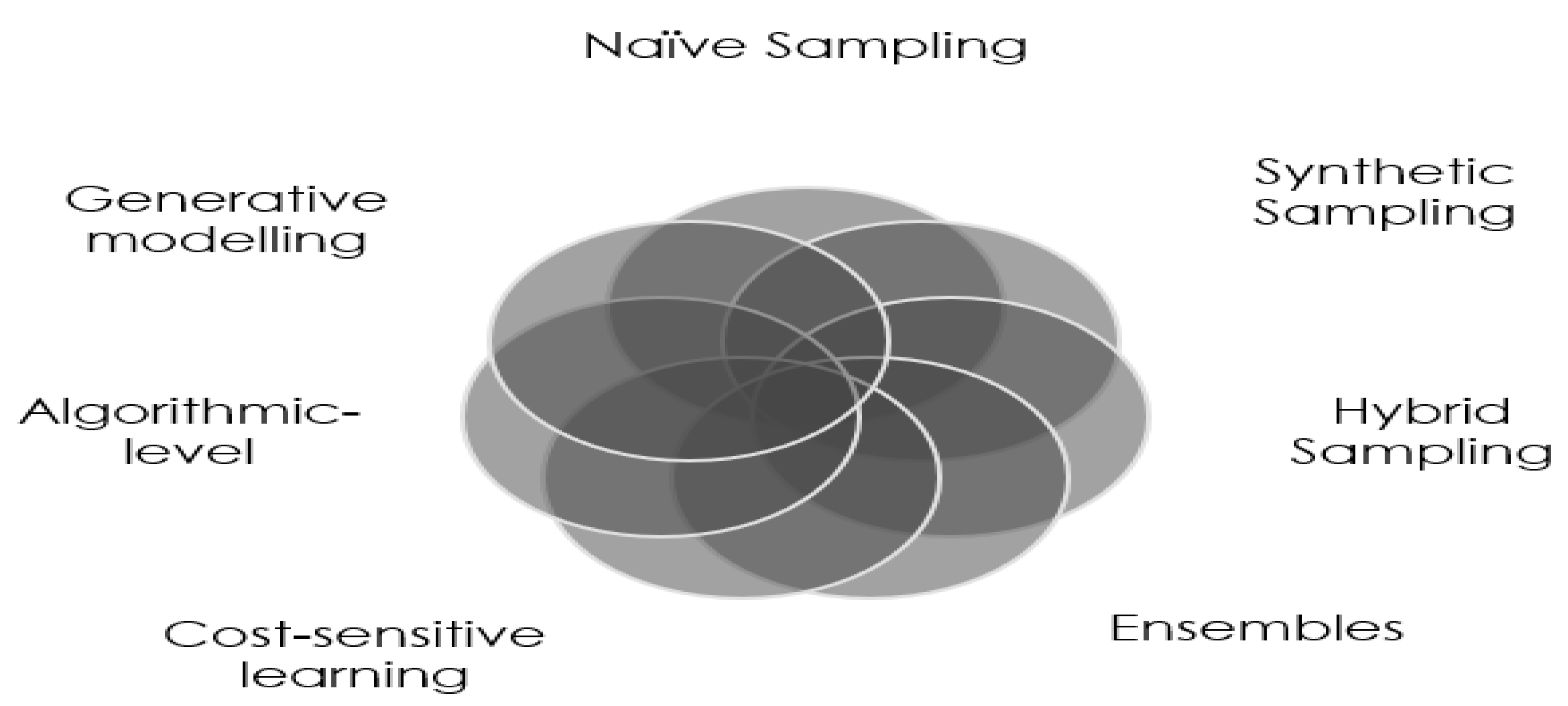
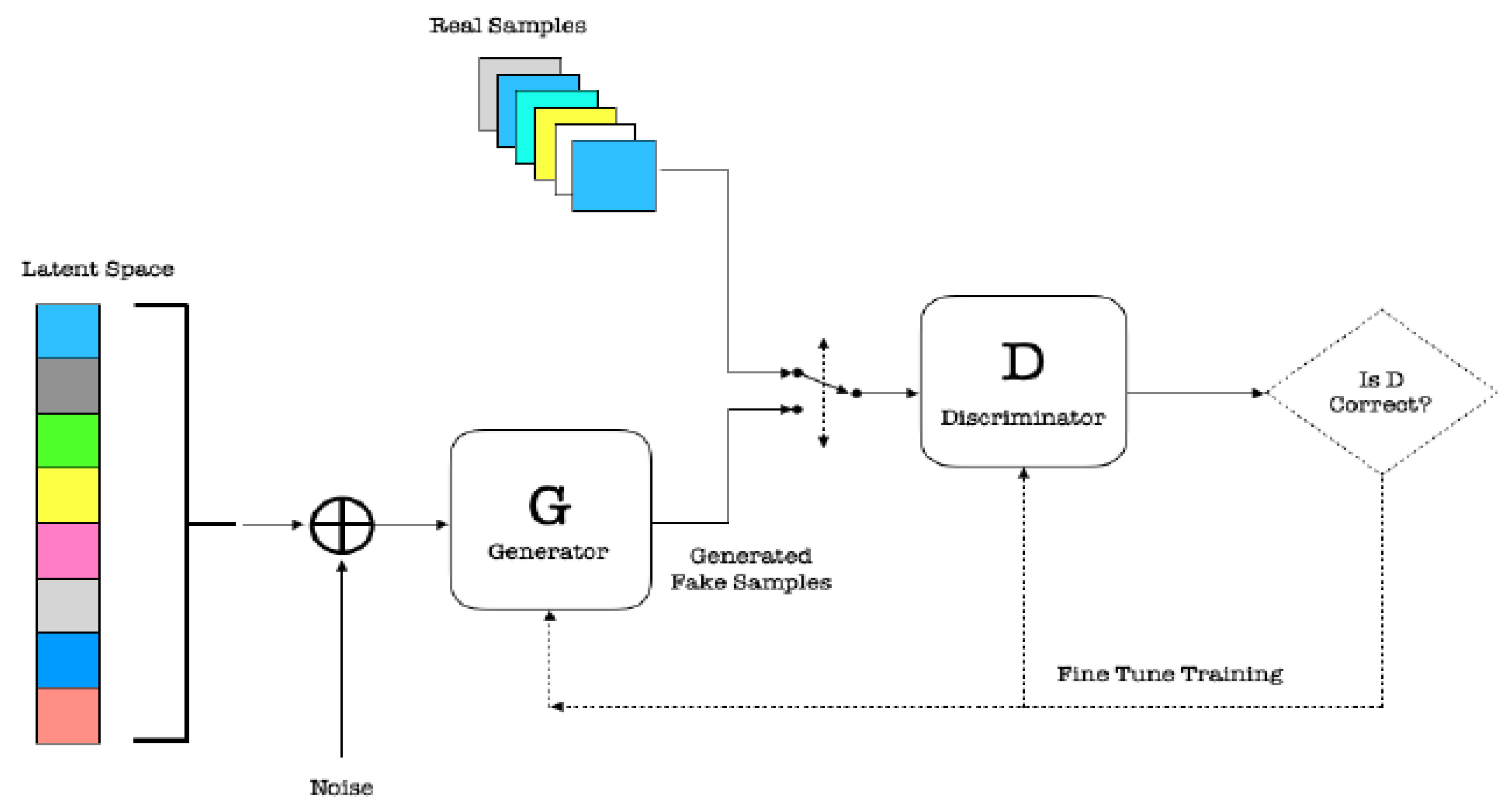
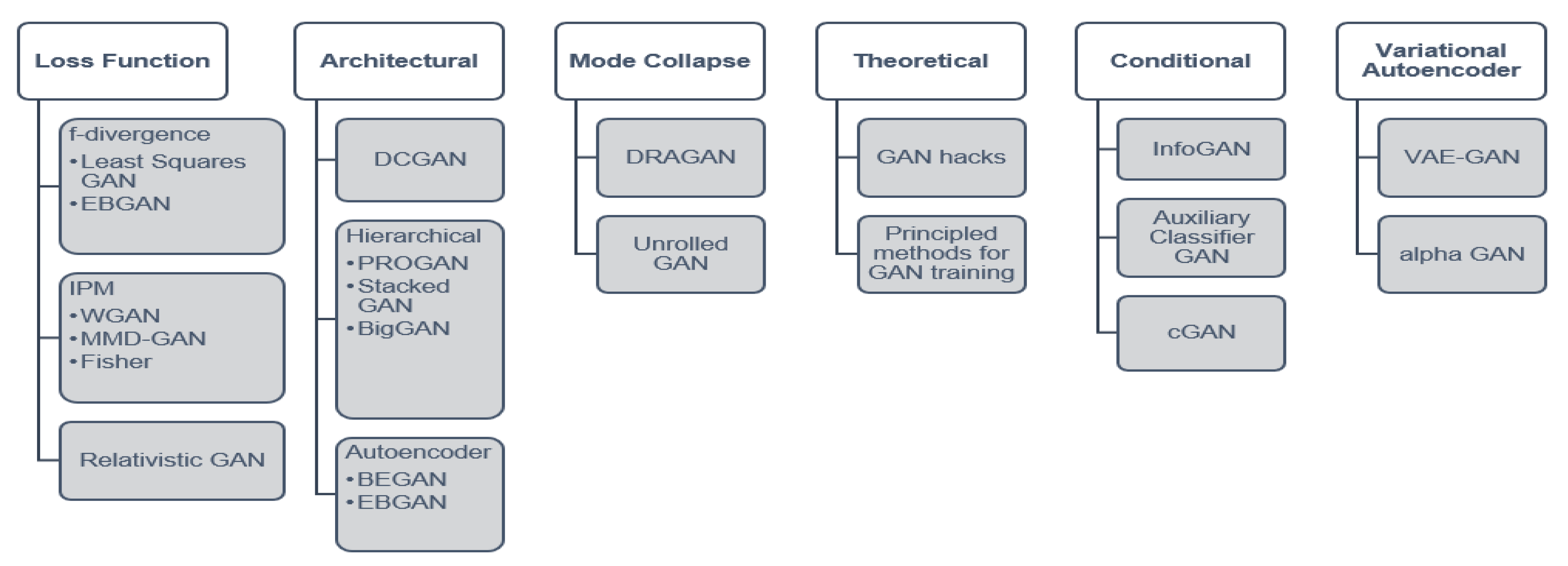
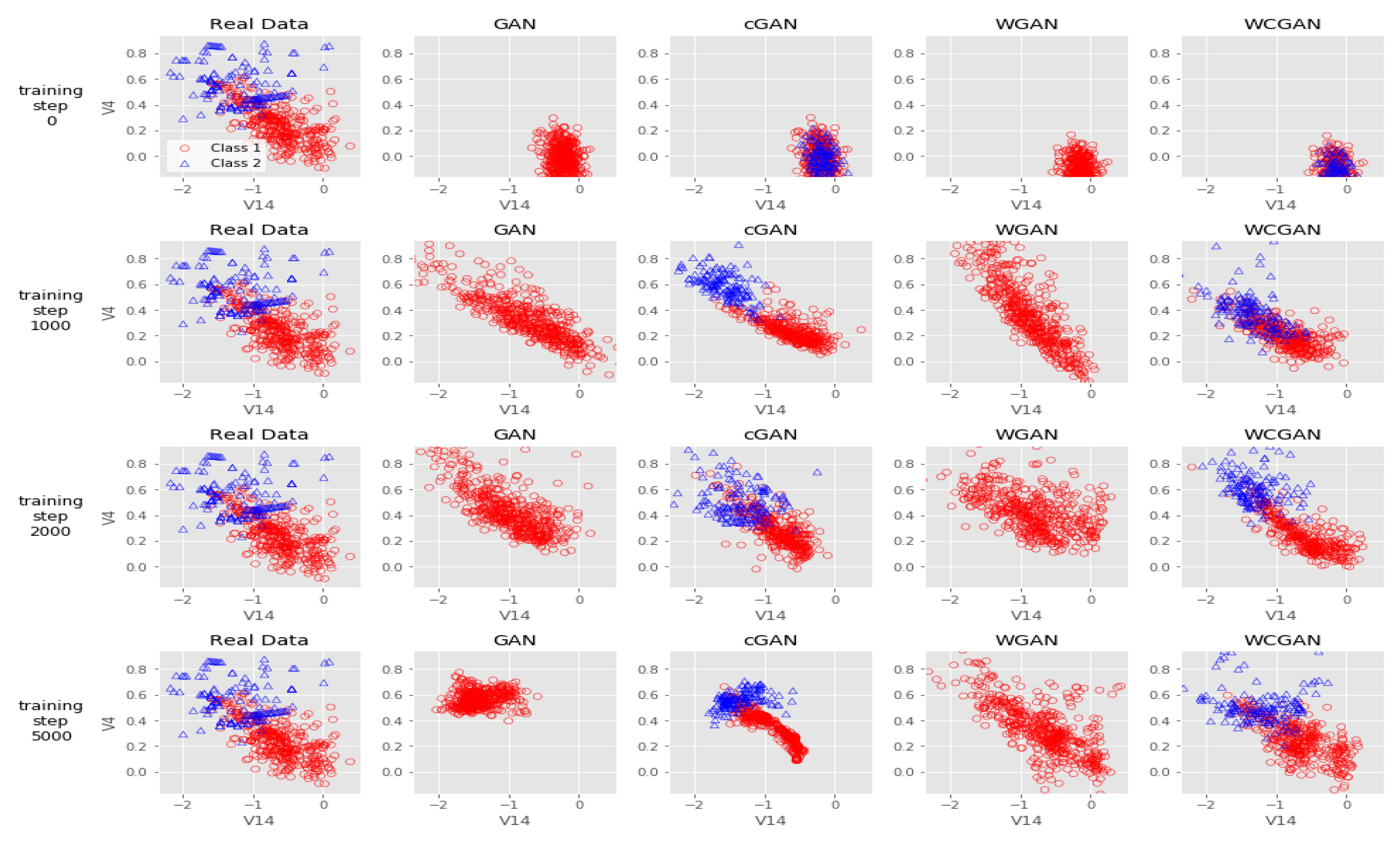
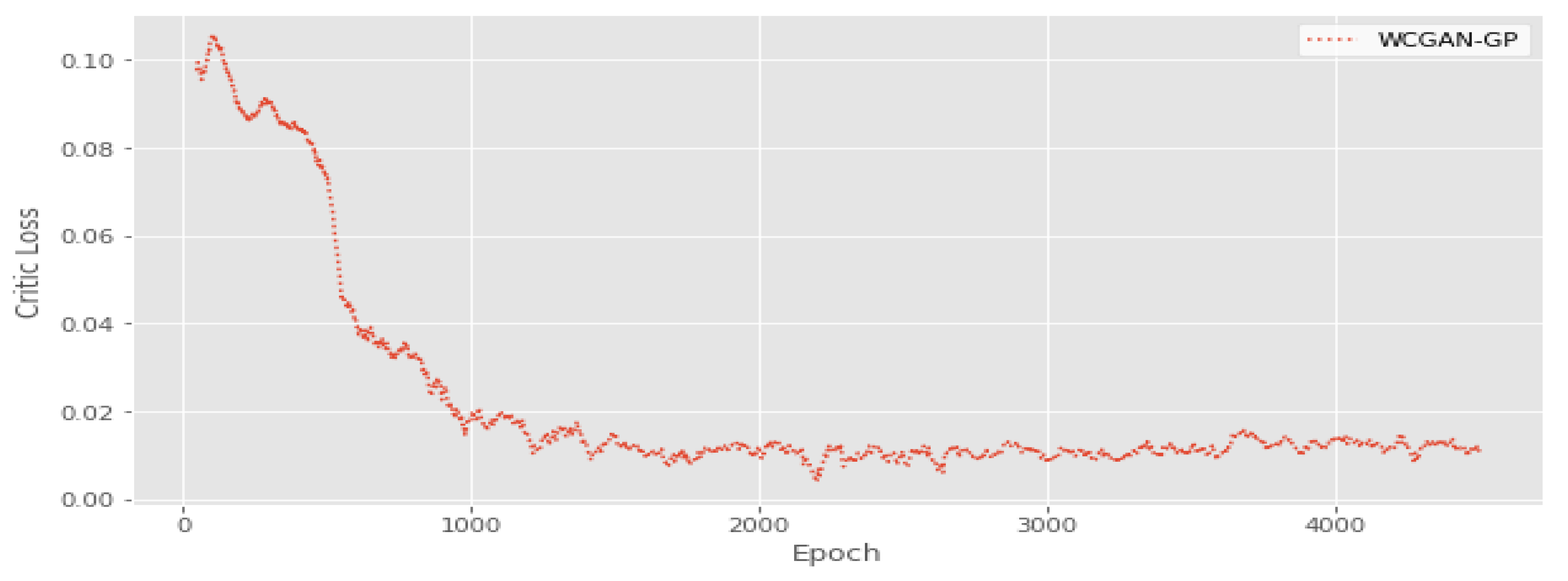
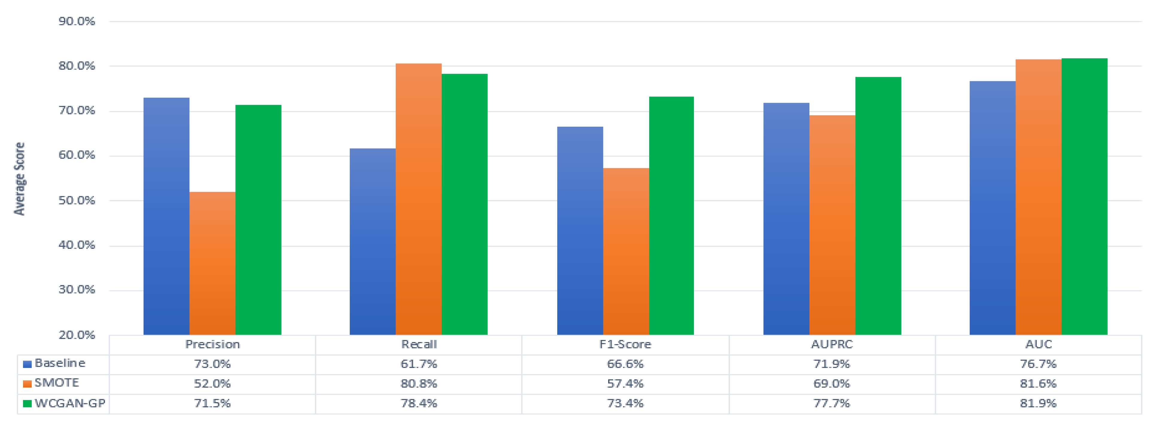
Table 1.
Taxonomy of generative models.
| Explicit Density | Approximate | Variational Inference | Variational Autoencoder |
| Markov chain | Deep Belief Network | ||
| Restricted Boltzmann Machine | |||
| Tractable | Full Visible Belief Net | NADE | |
| MADE | |||
| PixelRNN/CNN | |||
| Change of variable models | Nonlinear ICA | ||
| Implicit Density | Direct | Generative Adversarial Network | Minimax GAN |
| Non-saturating GAN | |||
| GAN variants | |||
| Generative Moment Matching Network | GMMN | ||
| Markov | Generative Stochastic Network | GSN |
Table 2.
Potential GAN applications in actuarial disciplines.
| Actuarial Discipline | Description |
|---|---|
| Product Design, Propensity and Customer Behavior | Create wider and more model points; Boost propensity models with more data per cell, leading to better and accurate models. |
| Actuarial Models | Experience monitoring and experience rates derived using a large credible data set. Boost models using data augmentation, semi-supervised learning, missing data imputation and domain adaptation for pricing, assumption setting, anomaly detection, risk estimation, time series and attention prediction in insurance, reinsurance, banking, investment, healthcare, and enterprise risk management. |
| Projections | Network modeling by looking at driving dependencies rather than correlation assumptions, i.e., use generative models. Strategic flexible and more decision-based models based on the environment. More GAN-based time series models driven by the environment. Enhanced solvency projection models and stress tests which are based on rich data sets. |
| Reserving | Make projections more predictive through a large enough credible data at all model points, i.e., accurate assumptions per risk cell with less margins. |
| Surplus Distribution | More granular individual information from alternative data sources through leveraging generative models. |
| Investment Strategy | Granular data for asset/liability modeling, i.e., use GANs to simulate scenarios that depend entirely on the adopted investment strategy and boosting the model. Enhanced market risk monitoring. Improvements to portfolio optimization. |
| Data Cleaning | Reduce errors; fill in gaps using imputation; increase the sample size; query other data sets and verify patterns using Cycle GANs. |
| Research | Make actuarial data sets more publicly available through synthesized data generated by GANs, boosting industry data. This is helpful for creating accurate and more up-to-date standard tables and encouraging actuarial research. |
| External Data Sources | Leverage other data sets through combining multiple data sets. For example, DualGAN or CycleGAN can be leveraged to learn a representation that encompasses different data sets. |
Table 3.
Imbalanced data sets used in the experiments.
| Imbalanced Data Set | Majority Cases | Minority Cases | Number of Features | Numeric Features | Ordinal Features |
|---|---|---|---|---|---|
| Credit Card Fraud | 284,807 | 492 | 31 | 31 | 0 |
| Pima Indians Diabetes | 500 | 268 | 8 | 8 | 0 |
| Glass Identification | 144 | 70 | 9 | 9 | 0 |
| German Credit Scoring | 700 | 300 | 20 | 14 | 6 |
| Breast Cancer Wisconsin | 357 | 212 | 28 | 28 | 0 |
Table 4.
Optimal parameter values for k-NN for each data set.
| Data Set | Value of k-NN |
|---|---|
| Credit Card Fraud | 6 |
| Pima Indians Diabetes | 9 |
| Glass Identification | 10 |
| German Credit Scoring | 12 |
| Breast Cancer Wisconsin | 10 |
| Parameter | Value |
|---|---|
Table 6.
The confusion matrix.
| Confusion Matrix | Predicted: Minority | Predicted: Majority |
|---|---|---|
| Actual: Minority | True Positive (TP) | False Negative (FN) |
| Actual: Majority | False Positive (FP) | True Negative (TN) |
Table 7.
Evaluation metrics for binary problems.
| Metric | Formula |
|---|---|
| Accuracy | |
| Precision | |
| Recall | |
| F1-Score | 2 |
Table 8.
Evaluation metrics based on a default threshold of .
| Method | Precision | Recall | F1-Score | AUPRC | AUC |
|---|---|---|---|---|---|
| Credit Card Fraud | |||||
| Baseline | |||||
| SMOTE | |||||
| WCGAN-GP | |||||
| Pima Indians Diabetes | |||||
| Baseline | |||||
| SMOTE | 53.54% | 80.30% | 64.24% | 68.18% | 75.48% |
| WCGAN-GP | |||||
| German Credit Scoring | |||||
| Baseline | |||||
| SMOTE | 47.83% | 70.51% | 56.99% | 58.84% | 69.61% |
| WCGAN-GP | |||||
| Glass Identification | |||||
| Baseline | |||||
| SMOTE | 73.91% | 70.83% | 72.34% | 87.29% | 72.86% |
| WCGAN-GP | 78.57% | ||||
| Breast Cancer Wisconsin | |||||
| Baseline | |||||
| SMOTE | 92.59% | 100.00% | 96.15% | 98.56% | 96.45% |
| WCGAN-GP |
Table 9.
Results for Friedman’s test.
| Data Set | p-Value | Significance |
|---|---|---|
| Credit Card Fraud | 2.9560 × | Yes |
| Pima Indians Diabetes | 0.188386 | No |
| German Credit Scoring | 1.0683 × | Yes |
| Glass Identification | 0.465622 | No |
| Breast Cancer Wisconsin | 4.0085 × | Yes |
Table 10.
Results for the post-hoc test.
| Test | Credit Card Fraud | German Credit | Breast Cancer |
|---|---|---|---|
| WCGAN-GP vs. SMOTE |
Publisher’s Note: MDPI stays neutral with regard to jurisdictional claims in published maps and institutional affiliations. |
© 2021 by the authors. Licensee MDPI, Basel, Switzerland. This article is an open access article distributed under the terms and conditions of the Creative Commons Attribution (CC BY) license (http://creativecommons.org/licenses/by/4.0/).
Share and Cite
MDPI and ACS Style
Ngwenduna, K.S.; Mbuvha, R. Alleviating Class Imbalance in Actuarial Applications Using Generative Adversarial Networks. Risks 2021, 9, 49. https://0-doi-org.brum.beds.ac.uk/10.3390/risks9030049
AMA Style
Ngwenduna KS, Mbuvha R. Alleviating Class Imbalance in Actuarial Applications Using Generative Adversarial Networks. Risks. 2021; 9(3):49. https://0-doi-org.brum.beds.ac.uk/10.3390/risks9030049
Chicago/Turabian StyleNgwenduna, Kwanda Sydwell, and Rendani Mbuvha. 2021. "Alleviating Class Imbalance in Actuarial Applications Using Generative Adversarial Networks" Risks 9, no. 3: 49. https://0-doi-org.brum.beds.ac.uk/10.3390/risks9030049
Note that from the first issue of 2016, this journal uses article numbers instead of page numbers. See further details here.