
Bayesian Mixture Modelling for Mortality Projection


1
Department of Actuarial Studies and Business Analytics, Macquarie University, Macquarie Park, NSW 2109, Australia
2
Faculty of Business Administration, Tokyo Keizai University, Tokyo 185-8502, Japan
*
Author to whom correspondence should be addressed.
Risks 2021, 9(4), 76; https://0-doi-org.brum.beds.ac.uk/10.3390/risks9040076
Submission received: 12 March 2021
/
Revised: 12 April 2021
/
Accepted: 12 April 2021
/
Published: 15 April 2021
(This article belongs to the Special Issue Mortality Forecasting and Applications)
Abstract
:Although a large number of mortality projection models have been proposed in the literature, relatively little attention has been paid to a formal assessment of the effect of model uncertainty. In this paper, we construct a Bayesian framework for embedding more than one mortality projection model and utilise the finite mixture model concept to allow for the blending of model structures. Under this framework, the varying features of different model structures can be exploited jointly and coherently to have a more detailed description of the underlying mortality patterns. We show that the proposed Bayesian approach performs well in fitting and forecasting Japanese mortality.
1. Introduction
In the demographic, actuarial, and insurance literature, the two main branches of mortality projection models are the Lee and Carter (1992) model family and the Cairns et al. (2006) (CBD) model family. There have been a large number of their variations, extensions, and applications to date (e.g., Lee 2000; Cairns et al. 2009; Haberman and Renshaw 2011). In most of these works, the selection of mortality projection models is mainly based on certain standard statistical criteria, such as the Akaike information criterion (AIC), Bayesian information criterion (BIC), mean square error (MSE), and mean absolute percentage error (MAPE). Once the “best model” is determined, the common practice is to simply apply the selected model singly to the problem under consideration (e.g., demographic projection, longevity risk pricing and hedging, capital assessment). While this approach is reasonably sound in its own right, it ignores the fact that there is still much uncertainty in actually how close the chosen model is to the true underlying mechanism and that the other suboptimal models may still capture useful aspects that are omitted by the selected model. It would be a serious waste if the other model candidates are simply discarded after putting in all the effort on fitting them to the data and only ranking them by a pre-specified, sometimes subjective, criterion.
There has been relatively little attention on a more proper assessment of the effect of model uncertainty. In this paper, we develop a fully Bayesian framework for incorporating multiple mortality projection models, including the Lee–Carter model, CBD model (with curvature), and age-cohort model. These models would depict different aspects of the data, and it would be useful to integrate them into a coherent framework. In particular, we employ the finite mixture model concept (e.g., Marin et al. 2005; Frühwirth-Schnatter et al. 2018) to estimate the probability of a model candidate and also blend the model structures in a formal manner. More specifically, the overall density function is expressed as a weighted average of the density functions of the individual components. Another perspective of using a finite mixture model is to take it as a semi-parametric approach that provides a more flexible way for handling complex data patterns, in contrast to simply applying a single model with limited features. Under such a framework, the distinct features of different model candidates can lead to a more thorough portrayal of the underlying mortality patterns. In effect, all of the inherent volatility, parameter uncertainty, and model uncertainty are allowed for simultaneously. Comparatively, previous studies in mortality projection generally took care of the first one or two uncertainties (via Monte Carlo simulation or bootstrapping) only. Moreover, the Bayesian approach allows joint estimation of the mortality structure and the time series structure, which avoids the potential estimation bias under the usual two-step procedure in fitting mortality projection models. Using Japanese mortality data, we show that the proposed Bayesian approach can give a better account of the uncertainty in model selection.
The other advantages of Bayesian modelling, in general, include the ability to cope with missing values and the room to embed relevant information into prior distributions. Earlier Bayesian mortality modelling work can be found in Czado et al. (2005), Pedroza (2006), Kogure et al. (2009), Cairns et al. (2011), Li (2014a, 2014b), and Van Berkum et al. (2017). Some applications in pricing or hedging longevity risk have been demonstrated by (Kogure and Kurachi 2010; Kogure et al. 2014), Cairns (2013), and Li et al. (2019).
The remainder of the paper is as follows. Section 2 introduces our Bayesian framework, which integrates the Lee–Carter model, the CBD model, and their time series processes, and presents the numerical results based on Japanese male mortality data. Section 3 sets out another Bayesian framework incorporating the Lee–Carter model and the age-cohort model and discusses the application results. Section 4 gives the concluding remarks.
2. Bayesian Lee–Carter with CBD
Let be the variables to be observed, be the future values of the variables, be the unknown parameters, and be the unknown weights of the model candidates. From a Bayesian perspective, the main objective is to deduce the joint posterior distribution , based on which different inferences can be drawn. The parameter estimates can be taken as the mean (or median) of the posterior distribution . The model candidate with the largest mean of can be regarded as the most probable or optimal model. The predictive distribution of the future values is then derived as . Within the Bayesian framework, the finite mixture model structure can be specified as , where denotes a density function, and the subscript refers to the ith model component. This mixture becomes particularly useful when the underlying data patterns are complicated and cannot be described sufficiently by one single model. In such a mixture, each model component would not just “compete” in making its own contributions to the overall description of the data features but also supplement the other model components by filling in their gaps.
Suppose is the central death rate at age in year . The first part is the Lee–Carter structure:
in which is the age effect, and is the period effect with age-specific sensitivity . The two identifiability constraints are and . The period effect is then modelled as a random walk with drift , where is the drift term and is the error term. The second part is the CBD structure with curvature:
where for year , is the level of the mortality curve, refers to the slope, is related to the curvature, is the average age, and is the average value of . The three time-varying parameters are then modelled as a three-dimensional random walk with drift , in which is the drift vector, and is the multivariate normal error vector with mean 0 and covariance matrix . The overall model’s density is then specified as below:
in which , and are the weights of the two components, and are the standard deviations of the two components, and is the standard normal density. It can be deduced that and .
The prior distributions of all the parameters above are assumed as follows:
The hyperparameters are chosen in such a way that the priors are as uninformative as possible. The uniform distribution of means that there is no preference over any of the two model structures at the start, assuming that there is no relevant prior information on the choice between them. The terms and are set to be 2.1, and and are set as 1.1 times the corresponding residual variances. The prior variances and are set as 10 times the sample variances of ’s and ’s (estimated via singular value decomposition) over age. The drift term mean and variance are computed from the estimated decrements . The term is assumed to be 2.1 and is taken as 1.1 times the sample variance of over time. The drift mean vector and covariance matrix are estimated from the trivariate decrements . The term is taken as times the sample covariance matrix of , and is set equal to 4. More details can be found in Kogure et al. (2009) and Li (2014b).
Since it is mathematically intractable to derive a closed-form solution for the joint posterior distribution, we use Markov chain Monte Carlo (MCMC) simulation to provide a random sample from the posterior, in which simulated samples are generated from a Markov chain having its stationary distribution equal to the posterior distribution (Spiegelhalter et al. 2003). We apply the software JAGS (Plummer 2017) to implement the MCMC simulations. It involves the Gibbs sampling method, which simulates from the fully conditional posterior distribution of each variable in sequence. The JAGS programming language operates on the R platform as a package. Note that while one may assume priors that are even more diffuse than those listed above, the computation time would then lengthen substantially, and the program may even crash.
For each run of the MCMC simulation, the initial 5000 iterations are discarded to remove the effect of the initial values, and afterwards, 1000 iterations are obtained. The collected 1000 scenarios are then used for estimating the parameters and probability intervals. As illustrated in the two examples in Figure 1, the resulting autocorrelations (bottom right) in the successive samples of each variable are negligible, which is a strong sign of proper convergence to the stationary distribution. Moreover, the Monte Carlo errors are largely around 5% or smaller of the sample standard deviations, providing further evidence on the convergence of the MCMC samples to the stationary distribution.
We have collected Japanese male mortality data of ages 60 to 89 and years 1970 to 2017 from the Human Mortality Database (HMD 2020) and fit the Lee–Carter model (only), the CBD model (only), and the mixture model to the data under the Bayesian framework as described above. During the data period, the mortality trends and patterns tend to be more complex for males than for females, so it would be interesting to apply the mixture model to the male data. Figure 2 compares the posterior means of , , , , , and from the Lee–Carter model alone or the CBD model alone against those from the mixture model. It can be seen that the parameter estimates of each structure have their basic shapes rather preserved under the mixture model.
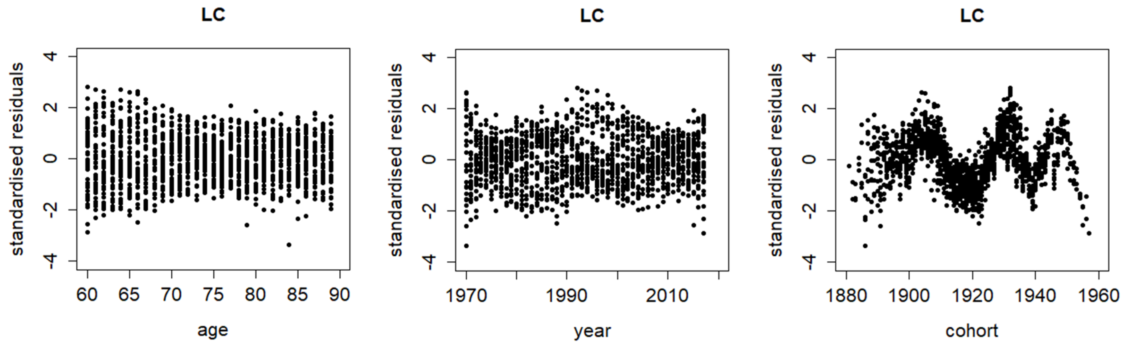
The posterior mean of in the Bayesian mixture model is 0.4398 with a standard deviation of 0.0224. This value suggests that the CBD structure is preferred over the Lee–Carter structure, as it is significantly different from 0.5 (with p-value of 0.01). However, it is still significantly larger than 0, which means that both structures, when used jointly, can potentially complement each other in describing the data. The deviance information criterion (DIC) is defined as the posterior mean of the deviance plus the effective number of parameters. The DIC values of applying the Lee–Carter, CBD, and mixture models are calculated as 20,552, 20,254, and 19,513, respectively. These statistics are in line with the two implications above—while the CBD model (alone) can be selected over the Lee–Carter model (alone), the mixture model actually gives the lowest DIC and is the optimal one amongst the three cases. The blending of the Lee–Carter and CBD structures clearly leads to an improvement in the fitting performance. It is also reflected in the residual graphs in Figure 3. There are distinctive patterns in the standardised residuals by cohort under the Lee–Carter model (alone) and by both age and cohort (to a lesser extent) under the CBD model (alone). These patterns are largely removed with the blending of the two structures (except for the more recent cohorts, as both structures have the same issue for that aspect of the data).
Figure 4 plots the log death rates at ages 60, 70, and 80 and their projected values (predictive means) to the year 2050 with 95% prediction intervals. It is interesting to observe that the mixture model generates the widest prediction intervals compared to the two single models. It can be regarded as a direct consequence of incorporating model uncertainty into the Bayesian modelling and simulations. Note that a proper allowance for all kinds of uncertainties is of critical importance in capital assessment and pricing and hedging of longevity risk (e.g., Haberman et al. 2014 and Li et al. 2017). In particular, the real impact of model uncertainty is often omitted in previous studies on longevity risk. Failure to take model uncertainty into full account could lead to a serious underestimation when valuing pensions and annuities and evaluating their risk allowances.
3. Bayesian Lee–Carter with Age-Cohort
Starting arguably from Renshaw and Haberman (2006), the cohort effect has become an important consideration in building a mortality projection model. It refers to unique mortality patterns that are found amongst only those individuals who were born in a given year. However, some authors (Cairns et al. 2009; Beutner et al. 2017) discussed the problems of slow convergence and lack of robustness and the identifiability issues when incorporating the cohort effect together with the period effect. Some possible solutions so far include using an alternative model structure (Haberman and Renshaw 2011) and different identifiability constraints (Hunt and Villegas 2015).
In this section, we explore a different treatment of the cohort effect in order to avoid the identifiability issues. In particular, the second part of the Bayesian framework in Section 2 is now replaced with the following age-cohort structure (Renshaw and Haberman 2006):
where is the age effect, and is the cohort effect with age-specific sensitivity . The two constraints required are and . The cohort effect is then modelled as a random walk with drift , in which is the drift term, and is the error term. The corresponding prior distributions are given below:
The hyperparameters are selected in the same way as in the previous section. Note that the Lee–Carter structure would fail to capture all the cohort effect, while this age-cohort structure would fail to capture all the period effect. They can then serve as a complement to each other, and their combination would take both the period and cohort effects into full account.
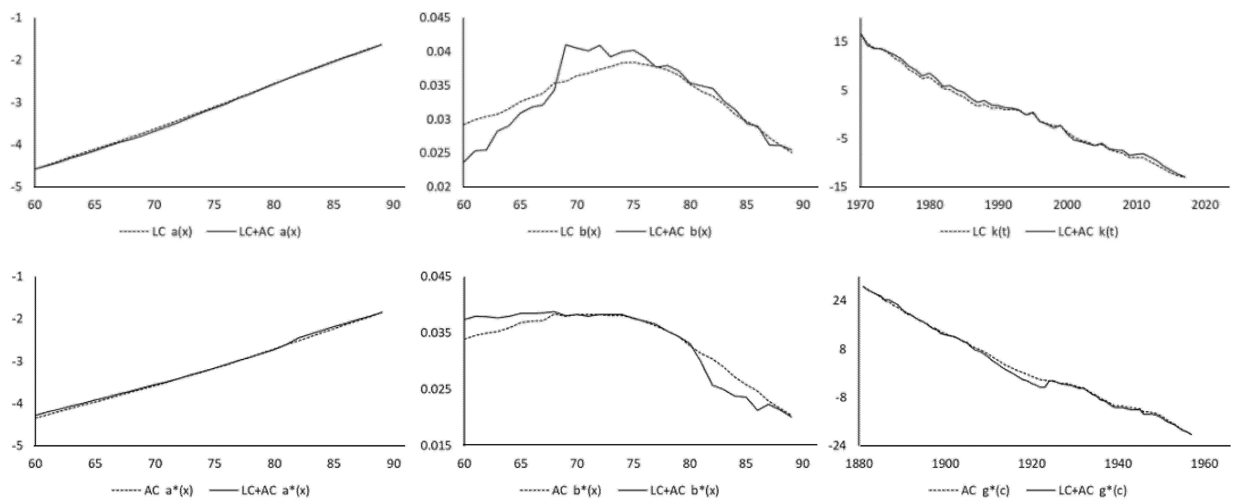
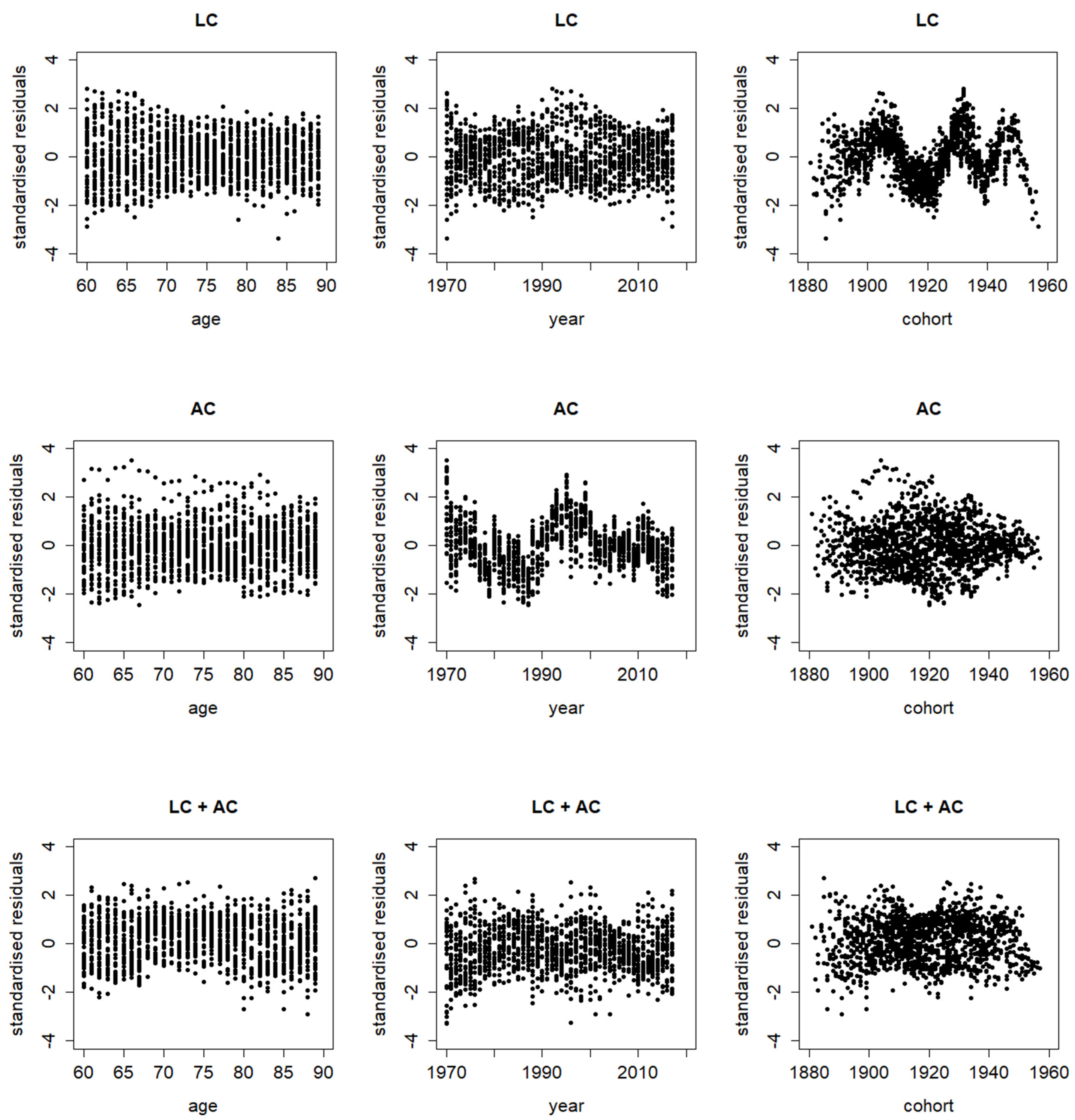
Figure 5 plots the posterior means of the parameters from the Lee–Carter model (alone), the age-cohort model (alone), and the mixture model. Again, the parameter estimates are quite similar between the single models and the mixture model. The posterior mean of in the mixture model is 0.4705 with a standard deviation of 0.0205. This time, the value of is not significantly different from 0.5 (with p-value of 0.15), which means that it is rather hard to select between the Lee–Carter and age-cohort structures. The DIC values of fitting the Lee–Carter, age-cohort, and mixture models are computed as 20,552, 20,644, and 19,709. The mixture model here (Lee–Carter with age-cohort) still delivers the lowest DIC amongst the three cases and so provides a better fitting performance than either of the two single models on its own, though it is slightly not as good as the one (Lee–Carter with CBD) in Section 2. Figure 6 compares the standardised residuals between the three cases. There are ripple patterns by cohort under the Lee–Carter model and by calendar year under the age-cohort model, which are understandable considering how the two single models allow for the period and cohort effects, respectively. Under the mixing of the two structures, by contrast, the residuals look much more randomly scattered, which means that the mixture model provides a better fit to the data.
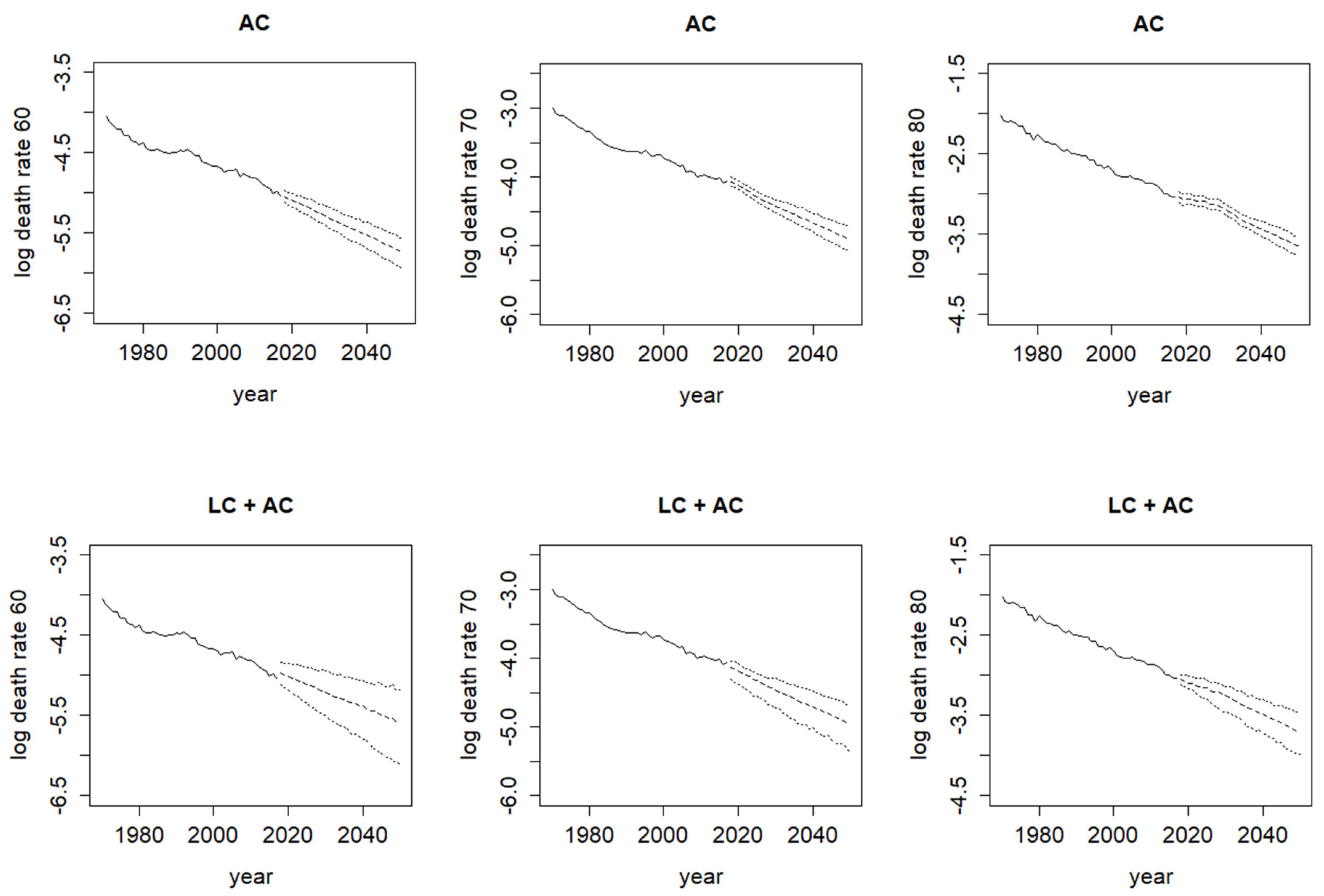
Figure 7 shows the corresponding log death rates at different ages with their projected values and prediction intervals. The mixture model here clearly produces much wider prediction intervals than those from the single age-cohort model. Again, these differences highlight the importance of allowing for model uncertainty adequately, or else there would be a nontrivial possibility of significantly underestimating the extent of longevity risk, leading to serious future financial losses for an annuity provider or a pension plan sponsor.
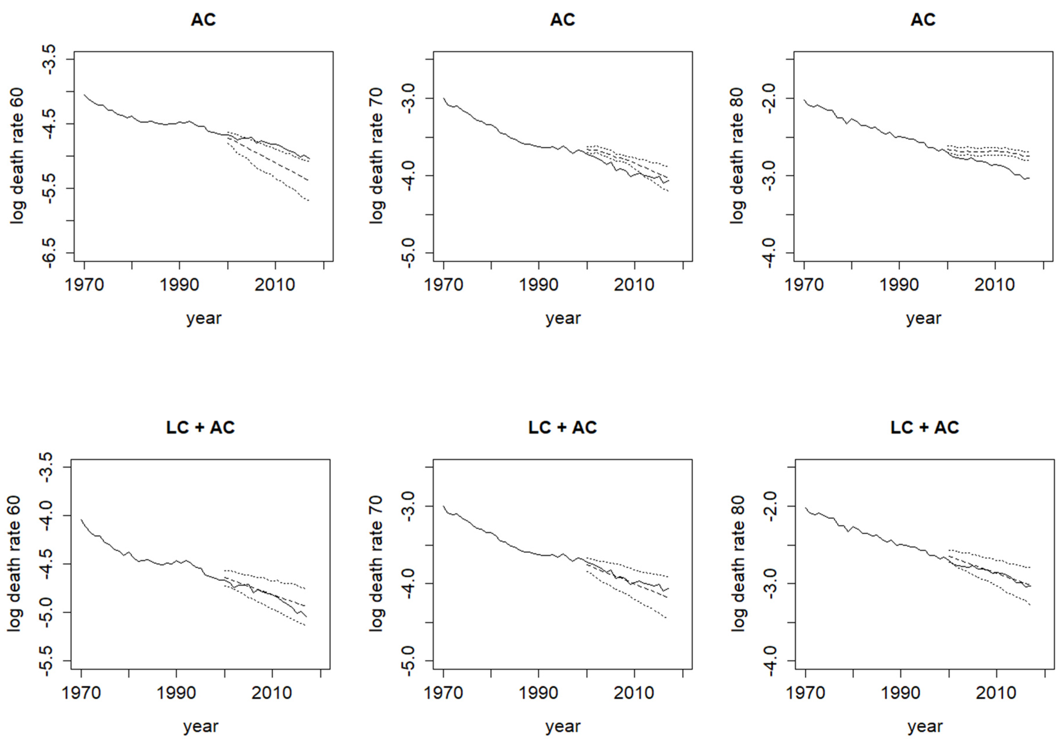
We then conduct an out-of-sample analysis and divide the data into two periods: 1970–1999 for fitting the models and 2000–2017 for assessing the forecast accuracy. For the Bayesian Lee–Carter, CBD, and age-cohort (single) models, and the two Bayesian mixture models, the mean absolute errors (MAE) of the projected log death rates over 2000–2017 are calculated as 0.0382, 0.0462, 0.1284, 0.0439, and 0.0363, respectively, as displayed in Table 1. It means that the Lee–Carter with age-cohort mixture model gives the best forecast accuracy while the single age-cohort model gives the worst performance. The corresponding mean square errors (MSE) are also in line with the MAE results. Figure 8 demonstrates the observed and simulated log death rates at different ages under these two models. As shown, the single age-cohort model fails to predict the mortality trends when compared with the Lee–Carter with age-cohort mixture model. For the former, not just the projected trends deviate much from the observed trends, but also the prediction intervals fail to capture the observed trends mostly. For the latter, by contrast, the observed trends lie well within the wider prediction intervals generally.
4. Concluding Remarks
In this paper, we devise a Bayesian framework for integrating multiple mortality projection model structures via the setting of a finite mixture model. In this framework, the different characteristics of the model components involved can be exploited in a joint and coherent manner in order to enhance the capacity in modelling complex mortality patterns. We demonstrate that the proposed Bayesian mixture modelling approach generates superior fitting and forecasting performances on Japanese mortality data when compared to the mere use of a single model. The new approach would lead to a more sufficient risk allowance in pension and annuity valuation. As the precise impact of model uncertainty is often overlooked in previous mortality projection studies, it is intended that this work would fill in some of the gaps in the current literature.
There are a few areas that would worth further research. First, three or more model structures can be combined altogether as a finite mixture model. It would be interesting to blend the Lee–Carter, CBD, age-cohort, and potentially many other models and test such a comprehensive mixture on various countries’ data; however, the computation time would then increase substantially as more structures are included. Second, the proposed approach can be extended to multi-population cases, such as both sexes, different socioeconomic classes or states in a country, and neighbouring countries. If one wants to ensure mortality coherence between the subpopulations, each of the model components in the mixture must possess the mortality coherence property itself.
Author Contributions
Methodology, J.L., A.K.; investigation, J.L., A.K.; writing—original draft preparation, J.L.; writing—review and editing, J.L., A.K.; funding acquisition, A.K. All authors have read and agreed to the published version of the manuscript.
Funding
Atsuyuki Kogure gratefully acknowledges financial support from JSPS KAKENHI Grant Numbers JP20K01777.
Institutional Review Board Statement
Not applicable.
Informed Consent Statement
Not applicable.
Data Availability Statement
Not applicable.
Conflicts of Interest
The authors declare no conflict of interest. The funder had no role in the design of the study; in the collection, analyses, or interpretation of data; in the writing of the manuscript, or in the decision to publish the results.
References
- Beutner, Eric, Simon Reese, and Jean-Pierre Urbain. 2017. Identifiability issues of age-period and age-period-cohort models of the Lee-Carter type. Insurance: Mathematics and Economics 75: 117–25. [Google Scholar] [CrossRef] [Green Version]
- Cairns, Andrew J. G. 2013. Robust hedging of longevity risk. Journal of Risk and Insurance 80: 621–48. [Google Scholar] [CrossRef]
- Cairns, Andrew J. G., David Blake, and Kevin Dowd. 2006. A two-factor model for stochastic mortality with parameter uncertainty: Theory and calibration. Journal of Risk and Insurance 73: 687–718. [Google Scholar] [CrossRef]
- Cairns, Andrew J. G., David Blake, Kevin Dowd, Guy D. Coughlan, and Marwa Khalaf-Allah. 2011. Bayesian stochastic mortality modelling for two populations. ASTIN Bulletin 41: 29–59. [Google Scholar]
- Cairns, Andrew J. G., David Blake, Kevin Dowd, Guy D. Coughlan, David Epstein, Alen Ong, and Igor Balevich. 2009. A quantitative comparison of stochastic mortality models using data from England and Wales and the United States. North American Actuarial Journal 13: 1–35. [Google Scholar] [CrossRef]
- Czado, Claudia, Antoine Delwarde, and Michel Denuit. 2005. Bayesian Poisson log-bilinear mortality projections. Insurance: Mathematics and Economics 36: 260–84. [Google Scholar] [CrossRef] [Green Version]
- Frühwirth-Schnatter, Sylvia, Gilles Celeux, and Christian P. Robert. 2018. Handbook of Mixture Analysis. Boca Raton: Chapman and Hall/CRC. [Google Scholar]
- Haberman, Steven, and Arthur Renshaw. 2011. A comparative study of parametric mortality projection models. Insurance: Mathematics and Economics 48: 35–55. [Google Scholar] [CrossRef] [Green Version]
- Haberman, Steven, Vladimir Kaishev, Pietro Millossovich, Andrés Villegas, Steven Baxter, Andrew Gaches, Sveinn Gunnlaugsson, and Mario Sison. 2014. Longevity Basis Risk: A Methodology for Assessing Basis Risk. Cass Business School, Hymans Robertson LLP, Institute and Faculty of Actuaries (IFoA), and Life and Longevity Markets Association (LLMA). Available online: https://www.actuaries.org.uk/system/files/documents/pdf/ifoa-llma-longevity-basis-risk-report.pdf (accessed on 1 December 2015).
- Human Mortality Database (HMD). 2020. University of California, Berkeley (USA) and Max Planck Institute for Demographic Research (Germany). Available online: https://www.mortality.org/ (accessed on 26 February 2020).
- Hunt, Andrew, and Andrés M. Villegas. 2015. Robustness and convergence in the Lee-Carter model with cohort effects. Insurance: Mathematics and Economics 64: 186–202. [Google Scholar] [CrossRef]
- Kogure, Atsuyuki, and Yoshiyuki Kurachi. 2010. A Bayesian approach to pricing longevity risk based on risk-neutral predictive distributions. Insurance: Mathematics and Economics 46: 162–72. [Google Scholar] [CrossRef]
- Kogure, Atsuyuki, Jackie Li, and Shinichi Kamiya. 2014. A Bayesian multivariate risk-neutral method for pricing reverse mortgages. North American Actuarial Journal 18: 242–57. [Google Scholar] [CrossRef]
- Kogure, Atsuyuki, Kenji Kitsukawa, and Yoshiyuki Kurachi. 2009. A Bayesian comparison of models for changing mortalities toward evaluating longevity risk in Japan. Asia-Pacific Journal of Risk and Insurance 3: 1–21. [Google Scholar] [CrossRef]
- Lee, Ronald D., and Lawrence R. Carter. 1992. Modeling and forecasting U.S. mortality. Journal of the American Statistical Association 87: 659–71. [Google Scholar] [CrossRef]
- Lee, Ronald. 2000. The Lee-Carter method for forecasting mortality, with various extensions and applications. North American Actuarial Journal 4: 80–93. [Google Scholar] [CrossRef]
- Li, Jackie, Atsuyuki Kogure, and Jia Liu. 2019. Multivariate risk-neutral pricing of reverse mortgages under the Bayesian framework. Risks 7: 11. [Google Scholar] [CrossRef] [Green Version]
- Li, Jackie, Leonie Tickle, Chong It Tan, and Johnny Siu-Hang Li. 2017. Assessing Basis Risk for Longevity Transactions—Phase 2. Macquarie University, Institute and Faculty of Actuaries (IFoA), and Life and Longevity Markets Association (LLMA). Available online: https://www.actuaries.org.uk/system/files/field/document/Longevity%20Basis%20Risk_Phase%202%20Report.pdf (accessed on 1 December 2017).
- Li, Jackie. 2014a. A quantitative comparison of simulation strategies for mortality projection. Annals of Actuarial Science 8: 281–97. [Google Scholar] [CrossRef]
- Li, Jackie. 2014b. An application of MCMC simulation in mortality projection for populations with limited data. Demographic Research 30: 1–47. [Google Scholar] [CrossRef] [Green Version]
- Marin, Jean-Michel, Kerrie Mengersen, and Christian P. Robert. 2005. Bayesian modelling and inference on mixtures of distributions. Handbook of Statistics 25: 459–507. [Google Scholar]
- Pedroza, Claudia. 2006. A Bayesian forecasting model: Predicting U.S. male mortality. Biostatistics 7: 530–50. [Google Scholar] [CrossRef] [PubMed]
- Plummer, Martyn. 2017. JAGS Version 4.3.0 User Manual. Available online: https://sourceforge.net/projects/mcmc-jags/ (accessed on 1 June 2019).
- Renshaw, Arthur, and Steven Haberman. 2006. A cohort-based extension to the Lee-Carter model for mortality reduction factors. Insurance: Mathematics and Economics 38: 556–70. [Google Scholar] [CrossRef]
- Spiegelhalter, David, Andrew Thomas, Nicky Best, and Dave Lunn. 2003. WinBUGS User Manual. Available online: https://www.mrc-bsu.cam.ac.uk/software/bugs/the-bugs-project-winbugs/ (accessed on 1 June 2004).
- Van Berkum, Frank, Katrien Antonio, and Michel Vellekoop. 2017. A Bayesian joint model for population and portfolio-specific mortality. ASTIN Bulletin 47: 681–713. [Google Scholar] [CrossRef] [Green Version]
Figure 1.
History plot (top left), posterior distribution function (top right), posterior density function (histogram; bottom left), and autocorrelation plot (bottom right) of (left panel) and (right panel), with two chains of simulations (pink and blue).
Figure 1.
History plot (top left), posterior distribution function (top right), posterior density function (histogram; bottom left), and autocorrelation plot (bottom right) of (left panel) and (right panel), with two chains of simulations (pink and blue).

Figure 2.
Posterior means of , , , , , and from Bayesian Lee–Carter model (alone), CBD model (alone), and mixture model.
Figure 2.
Posterior means of , , , , , and from Bayesian Lee–Carter model (alone), CBD model (alone), and mixture model.

Figure 3.
Standardised residuals by age, calendar year, and cohort year from Bayesian Lee–Carter model (alone), CBD model (alone), and mixture model.
Figure 3.
Standardised residuals by age, calendar year, and cohort year from Bayesian Lee–Carter model (alone), CBD model (alone), and mixture model.


Figure 4.
Log death rates at ages 60, 70, and 80 from 1970 to 2050 (solid—observed values; dashed—projected values; dotted—95% prediction intervals) under Bayesian Lee–Carter model (alone), CBD model (alone), and mixture model.
Figure 4.
Log death rates at ages 60, 70, and 80 from 1970 to 2050 (solid—observed values; dashed—projected values; dotted—95% prediction intervals) under Bayesian Lee–Carter model (alone), CBD model (alone), and mixture model.


Figure 5.
Posterior means of , , , , , and from Bayesian Lee–Carter model (alone), age-cohort model (alone), and mixture model.
Figure 5.
Posterior means of , , , , , and from Bayesian Lee–Carter model (alone), age-cohort model (alone), and mixture model.

Figure 6.
Standardised residuals by age, calendar year, and cohort year from Bayesian Lee–Carter model (alone), age-cohort model (alone), and mixture model.
Figure 6.
Standardised residuals by age, calendar year, and cohort year from Bayesian Lee–Carter model (alone), age-cohort model (alone), and mixture model.

Figure 7.
Log death rates at ages 60, 70, and 80 from 1970 to 2050 (solid—observed values; dashed—projected values; dotted—95% prediction intervals) under Bayesian age-cohort model (alone) and mixture model.
Figure 7.
Log death rates at ages 60, 70, and 80 from 1970 to 2050 (solid—observed values; dashed—projected values; dotted—95% prediction intervals) under Bayesian age-cohort model (alone) and mixture model.

Figure 8.
Log death rates at ages 60, 70, and 80 from 1970 to 2017 (solid—observed values; dashed—projected values; dotted—95% prediction intervals) under Bayesian age-cohort model (alone) and mixture model.
Figure 8.
Log death rates at ages 60, 70, and 80 from 1970 to 2017 (solid—observed values; dashed—projected values; dotted—95% prediction intervals) under Bayesian age-cohort model (alone) and mixture model.


Table 1.
Mean absolute errors (MAE) and mean square errors (MSE) of projected log death rates over 2000–2017 under different Bayesian models.
Table 1.
Mean absolute errors (MAE) and mean square errors (MSE) of projected log death rates over 2000–2017 under different Bayesian models.
| Model | MAE | MSE |
|---|---|---|
| Lee–Carter | 0.0382 | 0.0022 |
| CBD | 0.0462 | 0.0032 |
| age-cohort | 0.1284 | 0.0221 |
| Lee–Carter + CBD | 0.0439 | 0.0030 |
| Lee–Carter + age-cohort | 0.0363 | 0.0020 |
Publisher’s Note: MDPI stays neutral with regard to jurisdictional claims in published maps and institutional affiliations. |
© 2021 by the authors. Licensee MDPI, Basel, Switzerland. This article is an open access article distributed under the terms and conditions of the Creative Commons Attribution (CC BY) license (https://creativecommons.org/licenses/by/4.0/).
Share and Cite
MDPI and ACS Style
Li, J.; Kogure, A. Bayesian Mixture Modelling for Mortality Projection. Risks 2021, 9, 76. https://0-doi-org.brum.beds.ac.uk/10.3390/risks9040076
AMA Style
Li J, Kogure A. Bayesian Mixture Modelling for Mortality Projection. Risks. 2021; 9(4):76. https://0-doi-org.brum.beds.ac.uk/10.3390/risks9040076
Chicago/Turabian StyleLi, Jackie, and Atsuyuki Kogure. 2021. "Bayesian Mixture Modelling for Mortality Projection" Risks 9, no. 4: 76. https://0-doi-org.brum.beds.ac.uk/10.3390/risks9040076
Note that from the first issue of 2016, this journal uses article numbers instead of page numbers. See further details here.