
Modeling Best Practice Life Expectancy Using Gumbel Autoregressive Models


Interdiscliplinary Centre on Population Dynamics, University of Southern Denmark, 5000 Odense C, Denmark
Risks 2021, 9(3), 51; https://0-doi-org.brum.beds.ac.uk/10.3390/risks9030051
Submission received: 31 January 2021
/
Revised: 26 February 2021
/
Accepted: 2 March 2021
/
Published: 10 March 2021
(This article belongs to the Special Issue Mortality Forecasting and Applications)
Abstract
:Best practice life expectancy has recently been modeled using extreme value theory. In this paper we present the Gumbel autoregressive model of order one—Gumbel AR(1)—as an option for modeling best practice life expectancy. This class of model represents a neat and coherent framework for modeling time series extremes. The Gumbel distribution accounts for the extreme nature of best practice life expectancy, while the AR structure accounts for the temporal dependence in the time series. Model diagnostics and simulation results indicate that these models present a viable alternative to Gaussian AR(1) models when dealing with time series of extremes and merit further exploration.
1. Introduction
Best practice life expectancy (BPLE) (Oeppen and Vaupel 2002; Vallin and Meslé 2009) is the maximum life expectancy from among national populations during a given year, at a particular age. Since BPLE is just an annual maximum, Medford (2017) proposed to model it using extreme value theory (EVT). Since then, there have been interesting contributions surrounding the modeling and potential applications of BPLE from Liu and Li (2019) and Li and Liu (2020). Liu and Li (2019) used BPLE to approximate and extrapolate lower and upper bounds in life expectancy. Medford (2017) assumed that the dependencies between successive annual BPLEs were captured in time effects and fitted a time-varying generalized extreme value distribution (GEV), in effect a separate GEV for each year. However, Li and Liu (2020) explored a more sophisticated approach, using Archimedean copulas to account for the dependence based on the work of Wüthrich (2004). For detailed discussions of the issues around using EVT to fit BPLEs in practice, readers may refer to Medford (2017), which includes detailed exposition for the assumptions.
Gaussian models are the basic models for linear time series (Hamilton 1994; Harvey 1993). The underlying error process driving the series is assumed to have no autocorrelation, with a mean of zero and a constant variance. It is also not uncommon to additionally assume that the error process is itself Gaussian. Hence both the assumed innovations (error) and marginal distributions are often assumed to be normally distributed. However, in situations where data record extreme events, Gaussian time series are unsuitable.
In the context of Autoregressive integrated moving average (ARIMA) models, assuming GEV errors may be a reasonable assumption when modeling extremes: maxima or minima. Hughes et al. (2007) used the GEV to model innovations of time series of extreme Antarctic temperatures. However, there was no discourse around the stationary marginal distribution or any attempt to set it out explicitly. Toulemonde et al. (2010) used autoregressive models with a stationary marginal Gumbel extreme value distribution to model atmospheric methane and nitrous oxide levels. More recently, Balakrishna and Shiji (2014) applied a similar model to daily maxima of the Bombay Stock Exchange and the Standard and Poor’s Index.
The models employed by Balakrishna and Shiji (2014) and Toulemonde et al. (2010) were obtained by mixing extreme value distributions over a positive stable distribution: adding a Gumbel distributed variable to a positive -stable variable results in a Gumbel distributed variable too. This was previously highlighted by Crowder (1989); Hougaard (1986); Watson and Smith (1985) in the context of survival analysis. Tawn (1990) presented such models in the modeling of multivariate extremes, while Fougeres et al. (2009) did so in a mixture context. Other interesting applications are in Crowder (1998). Gumbel models were previously fit to BPLE (Liu and Li 2019; Medford 2017) but not with the modeling framework that we present here. The Gumbel distribution accounts for the extreme nature of BPLE, while the autoregressive (AR) structure accounts for the temporal dependence in the time series of BPLE. Theoretically, extreme value innovations are more suitable for time series of maxima than Gaussian innovations. We remain in the familiar ARIMA model framework but with some added complexity to reflect the extreme value marginal distributions from the innovations.
The aim of this paper is to present Gumbel autoregressive model of order one (Gumbel AR(1)) as an option for modeling BPLE, since they are not particularly well known, and much less widely used. They offer an alternative to modeling short-term dependencies among maxima coming from light-tailed distributions. We do not attempt to introduce new theory or methodology, as the focus is on demonstrating how this family of models can be straightforwardly applied and their advantages over traditional Gaussian AR models. We believe that these models merit further study and development and could be used in a range of contexts. This paper is structured as follows. Section 2 presents some background on the Gumbel distribution and stable distributions. Section 3 provides detail on the statistical basis of the Gumbel AR(1) model. Section 4 steps through the application of the model and Section 5 concludes.
2. Some Preliminaries
2.1. The Gumbel Distribution
The GEV distribution function is given by
defined on . The model is described by three parameters: , and referred to as the location, scale and shape parameters, respectively.
The shape parameter, , determines the heaviness of the right tail, and this leads to three types of distributions. When , the distribution has finite support and is short-tailed, leading to the Weibull distribution. When , there is polynomial tail decay, leading to heavy tails, and the GEV is of the Fréchet type. The case where is taken to be the limit of Equation (1), as and there is exponential tail decay leading to light tails, and the GEV is of the Gumbel type with distribution function
The characteristic function (cf) of the Gumbel distribution is given by
where is the gamma integral and is the complex number.
2.2. Positive -Stable Distributions
A random variable S is said to be -stable if for all non-negative real numbers and , there exist positive real numbers a and b such that + is equal in distribution to where and are independent, identically distributed (iid) copies of S. There are three cases where one can write down closed form expressions for the density and verify directly that they are stable. These are the normal, Cauchy and Lévy distributions. For other distributions, there are no closed form solutions.
The Gumbel AR model ultimately arises from the additive relationship between the Gumbel distribution and positive -stable variables.
Proposition 1.
Let S be an α-stable variable defined by its Laplace transform:
for all and . Let X be Gumbel distributed with parameters μ and σ and be independent of S. Then the sum is also Gumbel distributed with parameters μ and .
Proof.
The moment generating function of X is . Let . Y is obviously exponential-stable and has moment generating function (mgf) . Therefore, the mgf of is
which is the mgf of a Gumbel distribution with parameters and . □
3. Gumbel AR(1) Model
We begin with the framework of the simple stationary AR(1) model. Let a sequence of independent, identically distributed random variables be and define a stationary AR(1) sequence by
with and being independent. Suppose that where S is a positive stable random variable with the Laplace transform given in (4). Our goal is to have the marginal value of be an extreme value distribution of Gumbel type, as in Equation (2).
If F is the marginal distribution of in (6), a proper distribution for the innovation exists if and only if F is self-decomposable. The random variable X is self-decomposable if the ratio is also well-defined for all (). For the Gumbel AR(1) model this ratio is given by
Based on results from Brockwell and Brown (1978); Nolan (2020); Zolotarev (1986), it can be shown that has distribution where Z has the distribution −log. The mean and variance of the innovation random variable are given by
where is Euler’s constant. It follows then that
Various estimation methods are possible (Balakrishna and Shiji 2014), but we adopt a simple method of moments approach, similar in spirit to Toulemonde et al. (2010) in order to obtain estimates of the three unknown parameters of our Gumbel AR(1) model: , and . Therefore, we derive the following equations which we solve for and . Since are strictly stationary (Balakrishna and Shiji 2014; Toulemonde et al. 2010), we can write
leading to the method of moment estimators:
where and . We estimate using a Yule–Walker type estimate, since the method of moments cannot generate an estimator for it. Hence, in line with Toulemonde et al. (2010)
Note that and allows asymptotic standard errors to be estimated. The standard errors for and are rather more complicated, but details of them can be found in (Toulemonde et al. 2010).
4. Illustration
The data used in model implementation and testing came from two sources. First, the Human Mortality Database (HMD, 2020) (Human Mortality Database 2020) covers the low-mortality countries that have the best data and the highest life expectancies. It contains life tables for 41 countries plus all the raw data used in constructing those tables. The specific data used were life expectancy at birth for both males and females for the period 1965 to 2017. The second source of data was the United Nations world population prospects (United Nations Population Division 2019). This was used to supplement HMD data where they were not yet available for the most recent years (New Zealand, Taiwan, Canada and Israel) and to obtain the life expectancy for all the other countries and territories not found in the HMD. The choice of fitting period (1965 to 2017) was somewhat arbitrary, but was chosen in an attempt to strike a balance between using the most recent data and trends in BPLE (Liu and Li 2019; Vallin and Meslé 2009), and having sufficient data for reasonable parameter estimation.
To illustrate, we fit the AR(1) model with a Gumbel marginal distribution to time series of male and female best practice life expectancy at birth. The BPLEs which have been extracted from the data are presented in Figure 1.
We modeled the time series using standard ARIMA time series approaches. Since the time series trend upward, we first made it stationary. As the series evolves almost linearly and it was previously argued that the trend in BPLE is deterministic (Medford and Vaupel 2020), we achieved stationarity by subtracting the linear trend found by fitting a simple linear regression model. BPLE increased at about 0.21 years per annum for males and 0.22 years per annum for females in this data window.
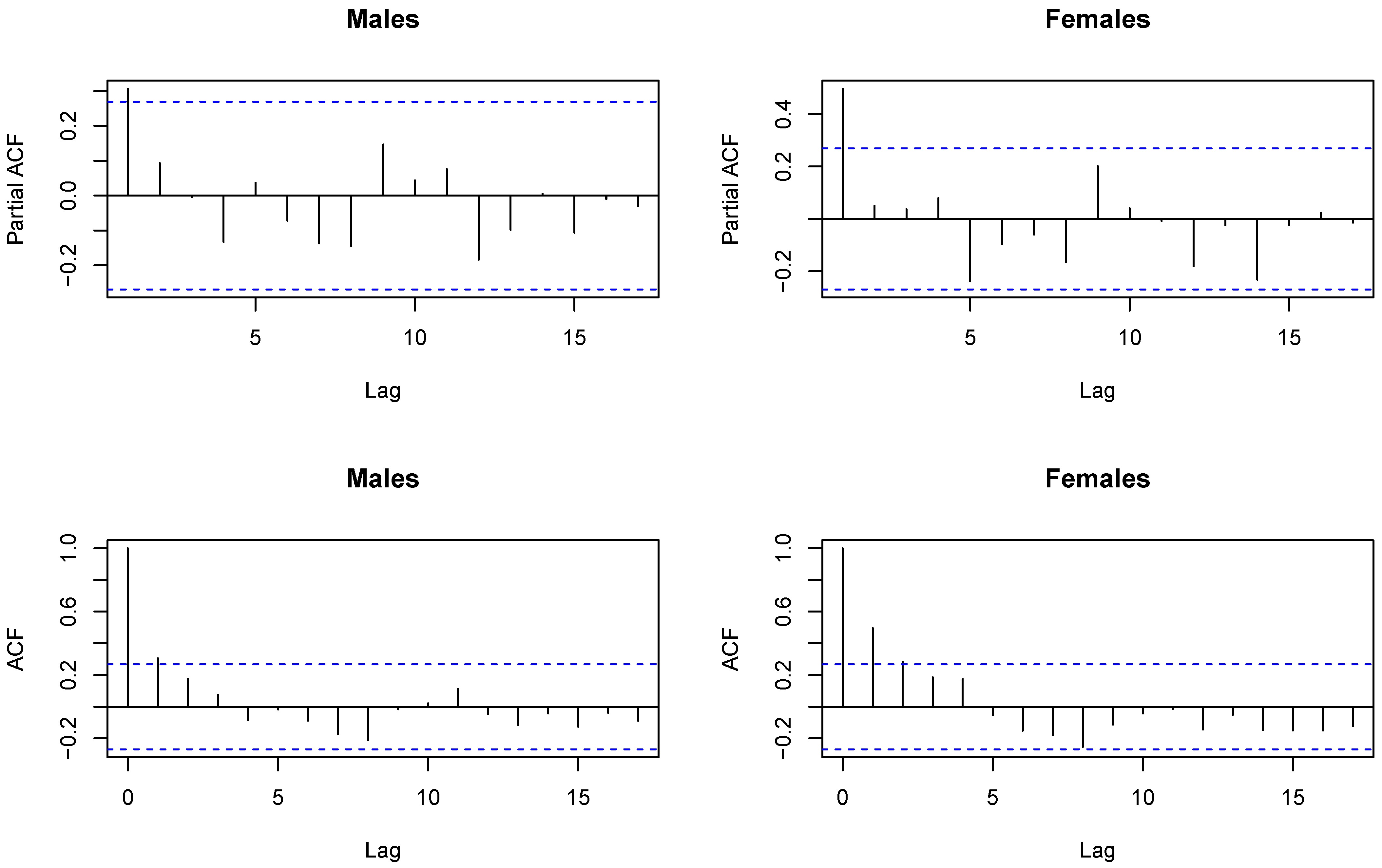
We needed to check the order of the fitted series and confirm that it has order one. We did this via the partial autocorrelation function (PACF). That is shown in Figure 2. In particular, the PACF cuts off at lag 1, suggesting that the autoregressive model of order 1 assumption is reasonable. An AR(1) model was also found to be the optimal model based on the AICc (corrected AIC) criterion.
The parameters , and were estimated using the method outlined in the previous section. These estimates, along with their standard errors, are presented in Table 1. Furthermore, the confidence interval for was (0.04, 0.56) for males and (0.24, 0.72) for females. Zero does not fall within these intervals, indicating that is a significant parameter and that the AR model may be appropriate.
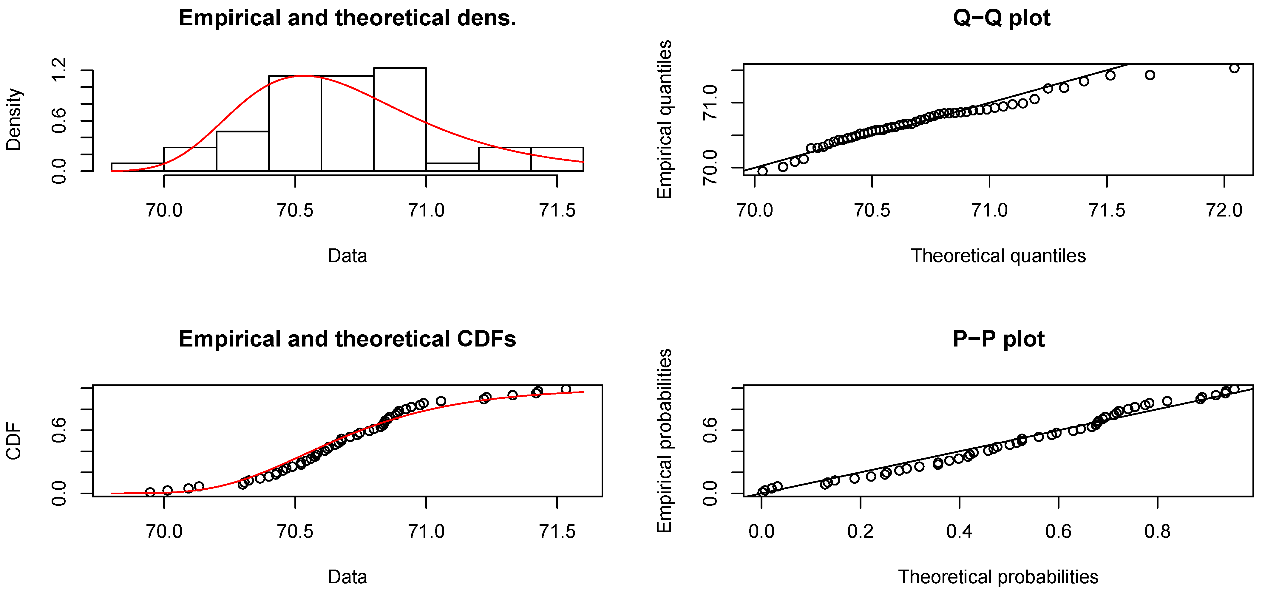
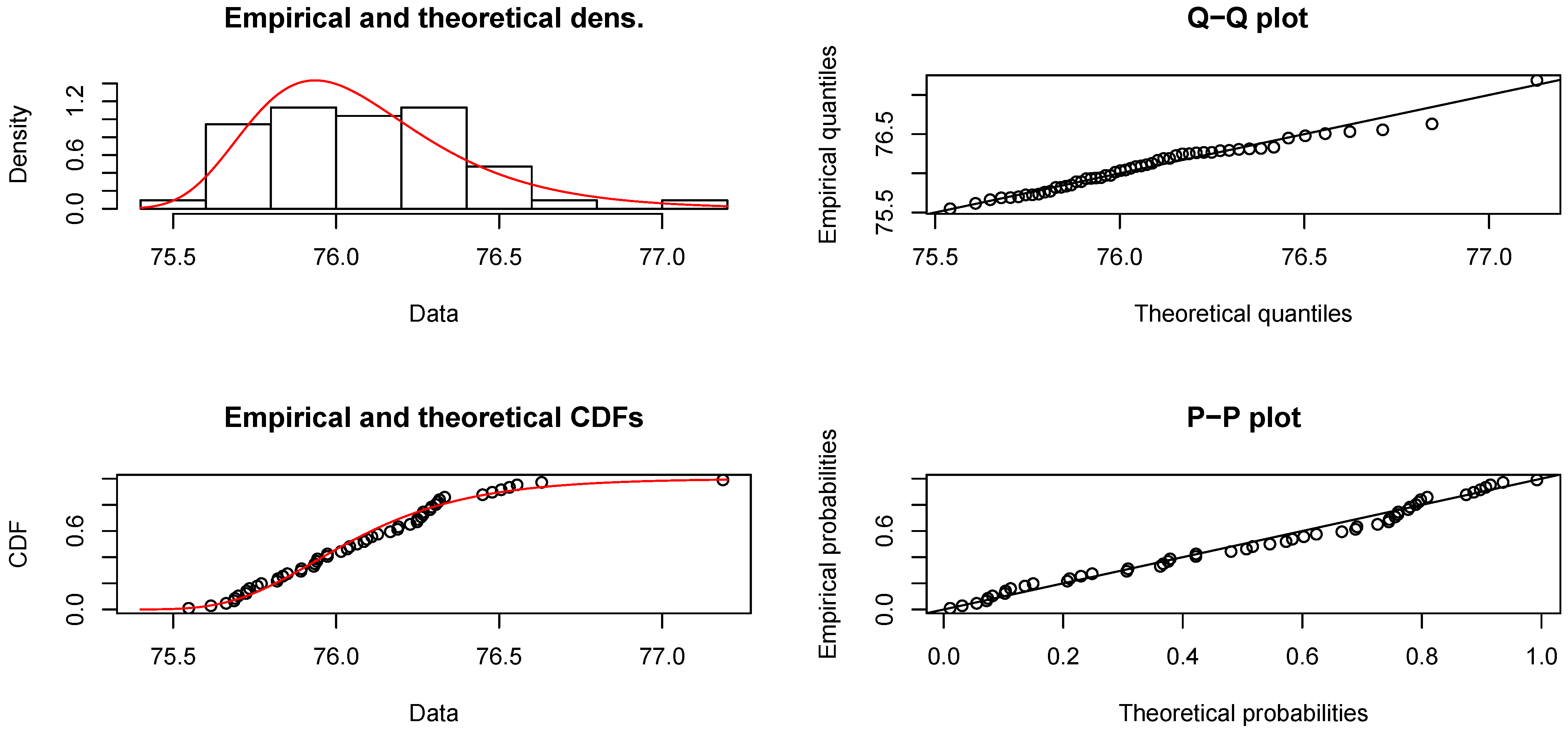
Appendix A presents diagnostics for the fitted model. The diagnostic tests confirm that an AR(1) model fits the time series well and that the Gumbel distribution is an acceptable choice for the marginal distribution. Therefore, we conclude that the Gumbel AR(1) model is adequate for the data.
A Comparison with Gaussian AR(1)
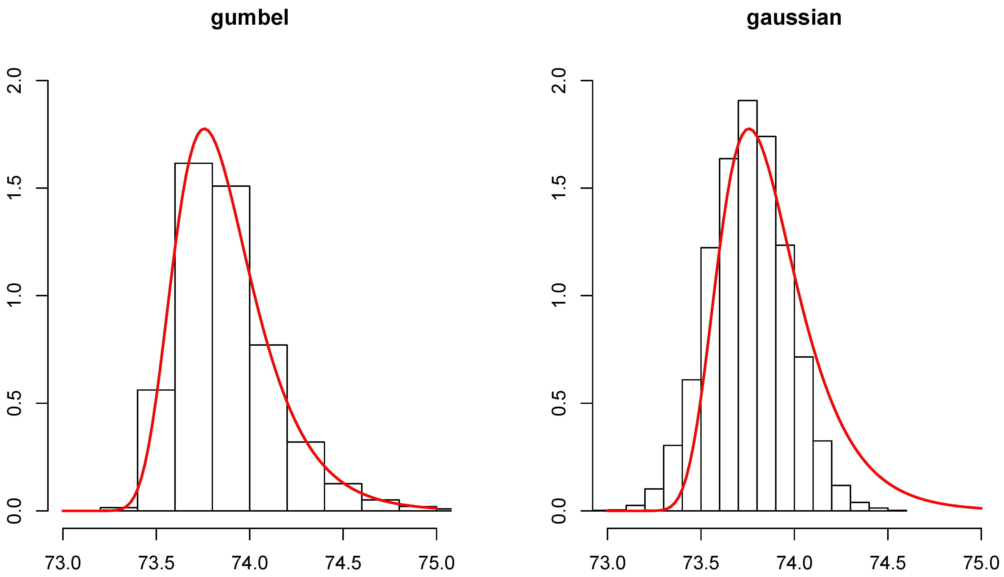
Given the extra effort involved in Gumbel AR(1) modeling, is it more accurate than using a Gaussian AR(1) model? The predictive distribution of in Equation (1) is a log positive -stable random variable (Toulemonde et al. 2010). Using the estimated parameters in Table 1, we simulated 10,000 observations from the fitted Gumbel AR(1) model and from a counter-factual Gaussian AR(1) model. We used a visual check of the histograms of the simulated observations from the two models which were then superimposed with the true Gumbel density. These comparisons are presented in Figure 3 and Figure 4. It is evident that the Gaussian distribution, because it is symmetric, fits the tails poorly and is unable to capture the asymmetry (short left tail, long right tail) in the data.
5. Conclusions
In this paper we presented a first-order Gumbel autoregressive model and fit it to a time series of best practice life expectancies. Gumbel AR(1) models can be used to model short term temporal dependence among extreme values which come from distributions that have reasonably light tails. The Gumbel AR(1) is rather limited, however, and it would be more appropriate to have greater flexiblity in the model. Greater flexibility includes, for example, being able to handle data with heavier tails and being able to fit different types of time series. A more general model should be able to fit the other extreme value distributions, the Frechet and Weibull distributions. It should also be able to accommodate the general class of ARIMA time series, not just AR(1) models. This opens up a potentially interesting area for future research. Forecasting using these types of models might also be an avenue that merits further exploration. In our view the usefulness and applicability of these models have not been fully explored and appear to be ripe for further development
Funding
The research and publication of this paper were supported by the AXA Research Fund, through the funding for the AXA Chair in Longevity Research.
Institutional Review Board Statement
Not applicable.
Informed Consent Statement
Not applicable.
Data Availability Statement
The data used in this study can be obtained from the Human Mortality Database, www.mortality.org and the United Nations 2019 Revision of World Population Prospects, https://population.un.org/wpp, accessed on 1 March 2021.
Acknowledgments
The author thanks Jana Vobecká and James W. Vaupel.
Conflicts of Interest
The authors declare no conflict of interest.
Appendix A
Figure A1.
Diagnostic plots to assess fit of Gumbel distribution: males.

Figure A2.
Diagnostic plots to assess fit of Gumbel distribution: females.

References
- Balakrishna, Narayana, and K. Shiji. 2014. Extreme value autoregressive model and its applications. Journal of Statistical Theory and Practice 8: 460–81. [Google Scholar] [CrossRef]
- Brockwell, Peter J., and B. Malcom Brown. 1978. Expansions for the positive stable laws. Zeitschrift für Wahrscheinlichkeitstheorie und Verwandte Gebiete 45: 213–24. [Google Scholar] [CrossRef]
- Crowder, Martin. 1989. A multivariate distribution with weibull connections. Journal of the Royal Statistical Society: Series B (Methodological) 51: 93–107. [Google Scholar] [CrossRef]
- Crowder, Martin. 1998. A multivariate model for repeated failure time measurements. Scandinavian Journal of Statistics 25: 53–67. [Google Scholar] [CrossRef]
- Fougères, Anne-Laure, John P. Nolan, and Holger Rootzén. 2009. Models for dependent extremes using stable mixtures. Scandinavian Journal of Statistics 36: 42–59. [Google Scholar] [CrossRef] [Green Version]
- Hamilton, James Douglas. 1994. Time Series Analysis. Princeton: Princeton University Press, vol. 2. [Google Scholar]
- Harvey, Andrew C. 1993. Time Series Models, 2nd ed. Birmingham: Harvester Wheatsheaf. [Google Scholar]
- Hougaard, Philip. 1986. A class of multivanate failure time distributions. Biometrika 73: 671–78. [Google Scholar] [CrossRef]
- Hughes, Gillian L., Suhasini Subba Rao, and Tata Subba Rao. 2007. Statistical analysis and time-series models for minimum/maximum temperatures in the Antarctic Peninsula. Proceedings of the Royal Society A: Mathematical, Physical and Engineering Sciences 463: 241–59. [Google Scholar] [CrossRef] [Green Version]
- Human Mortality Database. 2020. University of California, Berkeley (USA), and Max Planck Institute for Demographic Research (Germany). Available online: www.mortality.org (accessed on 15 January 2021).
- Li, Jackie, and Jia Liu. 2020. A modified extreme value perspective on best-performance life expectancy. Journal of Population Research 37: 345–75. [Google Scholar] [CrossRef]
- Liu, Jia, and Jackie Li. 2019. Beyond the highest life expectancy: Construction of proxy upper and lower life expectancy bounds. Journal of Population Research 36: 159–81. [Google Scholar] [CrossRef]
- Medford, Anthony. 2017. Best-practice life expectancy: An extreme value approach. Demographic Research 36: 989–1014. [Google Scholar] [CrossRef]
- Medford, Anthony, and James W. Vaupel. 2020. Extremes are not normal: A reminder to demographers. Journal of Population Research 37: 91–106. [Google Scholar] [CrossRef]
- Nolan, John P. 2020. Univariate Stable Distributions: Models for Heavy Tailed Data. Basingstoke: Springer Nature. [Google Scholar]
- Oeppen, Jim, and James W. Vaupel. 2002. Broken limits to life expectancy. Science 296: 1029–31. [Google Scholar] [CrossRef] [PubMed] [Green Version]
- Tawn, Jonathan A. 1990. Modelling multivariate extreme value distributions. Biometrika 77: 245–53. [Google Scholar] [CrossRef]
- Toulemonde, Gwladys, Armelle Guillou, Philippe Naveau, Mathieu Vrac, and Frederic Chevallier. 2010. Autoregressive models for maxima and their applications to CH4 and N2O. Environmetrics: The Official Journal of the International Environmetrics Society 21: 189–207. [Google Scholar]
- United Nations Population Division. 2019. World Population Prospects: The 2019 Revision. Volume I: Comprehensive Tables (ST/ESA/SER.A/379). New York: United Nations Population Division. [Google Scholar]
- Vallin, Jacques, and France Meslé. 2009. The segmented trend line of highest life expectancies. Population and Development Review 35: 159–87. [Google Scholar] [CrossRef]
- Watson, A. Smith, and Robert L. Smith. 1985. An examination of statistical theories for fibrous materials in the light of experimental data. Journal of Materials Science 20: 3260–70. [Google Scholar] [CrossRef]
- Wüthrich, Mario V. 2004. Extreme value theory and archimedean copulas. Scandinavian Actuarial Journal 2004: 211–28. [Google Scholar] [CrossRef]
- Zolotarev, Vladimir M. 1986. One-Dimensional Stable Distributions. Providence: American Mathematical Society, vol. 65. [Google Scholar]
Figure 1.
Best practice male and female life expectancies at birth, 1965–2017.

Figure 2.
Order checking of fitted time series. Top row: partial autocorrelation function. Bottom row: autocorrelation function.
Figure 2.
Order checking of fitted time series. Top row: partial autocorrelation function. Bottom row: autocorrelation function.

Figure 3.
Conditional histograms of for the Gumbel model and Gaussian model for males with superimposed Gumbel density based the estimated parameters.
Figure 3.
Conditional histograms of for the Gumbel model and Gaussian model for males with superimposed Gumbel density based the estimated parameters.

Figure 4.
Conditional histograms of for the Gumbel model and Gaussian model for females with superimposed Gumbel density based on the estimated parameters.
Figure 4.
Conditional histograms of for the Gumbel model and Gaussian model for females with superimposed Gumbel density based on the estimated parameters.


Table 1.
Estimated parameter values of a fitted Gumbel autoregressive model of order one—Gumbel AR(1) with estimated asymptotic standard errors.
Table 1.
Estimated parameter values of a fitted Gumbel autoregressive model of order one—Gumbel AR(1) with estimated asymptotic standard errors.
| Male | Female | |
|---|---|---|
| 0.30 (0.13) | 0.49 (0.12) | |
| 70.5 (0.05) | 75.9 (0.06) | |
| 0.27 (0.04) | 0.24 (0.04) |
Publisher’s Note: MDPI stays neutral with regard to jurisdictional claims in published maps and institutional affiliations. |
© 2021 by the author. Licensee MDPI, Basel, Switzerland. This article is an open access article distributed under the terms and conditions of the Creative Commons Attribution (CC BY) license (http://creativecommons.org/licenses/by/4.0/).
Share and Cite
MDPI and ACS Style
Medford, A. Modeling Best Practice Life Expectancy Using Gumbel Autoregressive Models. Risks 2021, 9, 51. https://0-doi-org.brum.beds.ac.uk/10.3390/risks9030051
AMA Style
Medford A. Modeling Best Practice Life Expectancy Using Gumbel Autoregressive Models. Risks. 2021; 9(3):51. https://0-doi-org.brum.beds.ac.uk/10.3390/risks9030051
Chicago/Turabian StyleMedford, Anthony. 2021. "Modeling Best Practice Life Expectancy Using Gumbel Autoregressive Models" Risks 9, no. 3: 51. https://0-doi-org.brum.beds.ac.uk/10.3390/risks9030051
Note that from the first issue of 2016, this journal uses article numbers instead of page numbers. See further details here.