
A Data-Driven Identification Procedure for HVAC Processes with Laboratory and Real-World Validation


1
Institute of Automation, Measurement and Applied Informatics, Faculty of Mechanical Engineering, Slovak University of Technology in Bratislava, 812 31 Bratislava, Slovakia
2
Prosystemy, s.r.o. (Ltd.), 900 86 Budmerice, Slovakia
*
Author to whom correspondence should be addressed.
Processes 2022, 10(1), 83; https://0-doi-org.brum.beds.ac.uk/10.3390/pr10010083
Submission received: 30 November 2021
/
Revised: 19 December 2021
/
Accepted: 24 December 2021
/
Published: 31 December 2021
(This article belongs to the Special Issue Emerging Technologies in Heating, Ventilation, Air Conditioning and Refrigeration (HVAC&R) Systems)
Abstract
:Linear system identification is a well-known methodology for building mathematical models of dynamic systems from observed input–output data. It also represents an essential tool for model-based control design, adaptive control and other advanced control techniques. Use of linear identification is, however, often limited to academic environment and to research facilities equipped with scientific computing platforms and highly qualified staff. Common industrial or building control system technology rarely uses these advanced design techniques. The main obstacle is typically lack of experience with their practical implementation. In this article, a procedure is proposed, implemented, and tested, that brings the benefits of linear identification into broader control system practice. The open-source DCU control system platform with its advanced control framework is used for implementation of the proposed linear identification procedure. The procedure is experimentally tested in the laboratory setting using a unique model of HVAC system as well as in real-world environment in an experimental two storey family house. Testing this novel feature of the control system has proved satisfactory results, while some of them are presented in graphical and numerical form.
1. Introduction
Smart building solutions, green building technology or Industry 4.0 are nowadays popular and frequently mentioned terms [1]. They refer to a general idea, that Heating, Ventilation and Air-Conditioning (HVAC) technologies in buildings, production lines in factories or even standalone machines shall be more intelligent in some way. This intelligence is supposed to bring fully automated, more cost-effective and more reliable operation with comfortable and intuitive Human-Machine Interface (HMI). The request is addressed mainly to control system engineering even if the information technology (IT) engineering is trying to address the problem as well. IT sector is, in consequence, asserting different concepts, such as Internet of Things (IoT), into the control system domain.
In spite of smart control trend, in common control system practice the ‘smart’ system typically ends up to be a standard control system augmented with an additional package of communication protocols, sensors, detectors and actuators. More auxiliary processes are automated and more process data is collected and logged, but the issue with the data except for control and displaying in tables and graphs remains unclear. We believe that control system engineering shall focus on implementation of advanced control system techniques into common practice.
By advanced control system techniques we mean all methods of control system theory not used in common control engineering practice. This includes linear system identification, model-based controller design, robust control, adaptive control, fault detection and fault-tolerant control, model predictive control, etc. All these techniques are well developed and documented, including studies focused on HVAC systems in smart buildings, see e.g., [2,3,4,5]. However, their use is still mostly limited to the academic environment—universities, research laboratories and R&D centres of large companies. Moreover, these techniques are typically applied in specific case studies rather than in common practical control setups. This is mainly due to the fact that the implementation of advanced control techniques is not straightforward and requires highly qualified and experienced staff.
1.1. Motivation
To implement advanced control techniques into common control system practice, the aforementioned methods must become an integral part of a specific control system platform. These techniques also must be correctly pre-set in advance or have an auto-tuning capability so that an ordinary control engineer does not need all knowledge and experience for their reliable use. Control engineering practice is inherently dealing with a large amount of practical issues from wiring through programming of process control down to installing of Supervisory Control And Data Acquisition (SCADA) servers. Budget for advanced control is, however, modest in most small and medium research companies. Therefore, activating or setting up an advanced technique must be a matter of a few clicks. Parameters to set, if any, must be related to practical control issues understandable to the control engineer and not to the internal behaviour of the given technique.
This article proposes a novel practical procedure that implements linear system identification techniques [6] and that is integrated into an open-source Dynamic Control Unit (DCU) platform. This platform is particularly suitable for integration of advanced techniques. Its implementation framework is a support software package developed for the DCU and it is called Advanced Supervision Server (ASServer). The framework has a dedicated interface that allows using of advanced techniques programmed directly in Scilab or MATLAB numerical computing platforms. This allows various control system toolboxes used or developed at universities (typically in MATLAB/Simulink, Scilab/Xcos) to be directly implemented without re-programming. Our recent publication [7] shows an experimental implementation of frequency anomalies detection tool into this platform. The use of fully open-source platforms is a relevant motivation for the authors to provide such tools not only to control practitioners, but to technical enthusiasts and public in general.
In this study we emphasise the HVAC as a case study for the identification procedure. Note that an appropriate identification of the HVAC processes in buildings is essential to design an adequate, cost-effective and easily implementable control scheme that ensures effective and reliable service. The proposed procedure is tested in simulation, in experiments with laboratory HVAC system as well as with the real-world HVAC technology in a building.
Proper modelling of HVAC systems is a field that requires a great attention for several reasons which are based mainly on the fact that buildings are considered as the biggest consumers worldwide (35% of total energy in 2018–2019 and 36% in 2020 [8,9,10]). To be more specific, let us divide energy consumption into four sectors, for which the consumed amount is specified as follows—residential (22%), non-residential (8%), industrial (38%) and transportation (28%)—in 2018 [8] as well as in 2019 [9]. Due to the economic slowdown caused by the COVID-19 pandemic, energy demand shifted from the commercial sector to the residential sector in 2020 [10]. Based on the statistical data [11], a significant portion of consumed energy is used to achieve thermal comfort of occupants; this relates mainly to space heating and cooling. Therefore, it is really a good and valid motivation to minimise energy consumption of buildings, especially the heating/cooling part, taking into account the fact that people spend majority of their lives indoors. The aim behind implementing advanced techniques is to decrease energy consumption and to achieve a satisfactory level of comfort for residents simultaneously. This can be accomplished by a better sensing of all relevant information and by designing suitable control algorithms based on the best possible model of a particular building.
1.2. HVAC Processes Identification
Generally, for designing adequate control loops to increase efficiency of these systems, it is necessary to have a good model of the plant, which can be obtained by a well-designed identification procedure. Since HVAC systems and buildings in general are complex systems, this can be very challenging [12] to model, therefore, such system can be divided into several sub-models. Obtaining appropriate models requires knowledge of the underlying physical phenomena of the system or huge amount of measured data. Based on this, there are three basic approaches—physics-based model (white-box), data-driven (black-box) and hybrid (grey-box) modelling.
It is well known that a white-box model comes from the first principles, thus requires knowledge of the process and the equations that describe it. This type of model is easy to analyse and has good generalisation capability, however, it has poor accuracy. On the contrary, in data-driven modelling the knowledge of mathematical model is not required. The underlying empirical model depends only on the measured values of the input/output variables. Consequently, it is necessary to have a lot of informative data available. A disadvantage of this approach is low generalisation and worse reliability in terms of reflecting the physical behaviour of the system. These statements are supported by many scientific publications and specialised books (e.g., [6,12,13,14]). Finally, the grey-box approach naturally combines the advantages of the aforementioned.
From a historical point of view, the heat conduction equation, published in 1822 by Joseph Fourier, is a pioneer in terms of modelling the HVAC processes. The work [12] discusses also another approach of modelling based on Stephenson’s and Mitalas’s simulations, which were built on response factor methods. Subsequently, heat balanced approaches were introduced in 1970’s. A more complex approach to HVAC modelling, introduced one decade later were the transient models. Evolving from these, two main groups were classified—steady-state models, in which the parameters are constant, and unsteady-state models, where the parameters are varying in time [13].
Table 1 provides a summary and brief comparison of modelling techniques proposed for HVAC systems, in terms of some relevant criteria, pros and cons of individual modelling approaches, etc. We refer an interested reader to the review articles of Afram’s and Janabi-Sharifi’s [15] and Afroz’s et al. [13] for a comprehensive overview. See also [16] for an up-to-date review of data-driven techniques for identification of HVAC systems.
In our case, it will be a black-box method and thus the construction of the model and the identification of parameters will depend only on the measured input and output data from the process. Such an approach to identification is often used in the field of building automation (see e.g., [17,18,19,20,21,22]). The implementation of online system identification stems not only from the need for advanced control techniques (e.g., in [23]) and other reasons discussed above, but also from the experience of employees of the Prosystemy company who work as operators and building managers.
2. Materials and Methods
In the following we present an advanced procedure for autonomous online linear system identification in the process control environment. An experimental and practical validation of this procedure is shown as well. The practical implementation is done in the open-source Global Monitoring Control System (GMCS) platform based on the DCU real-time hardware. The GMCS platform is particularly suitable for implementation of advanced control methods as it integrates Global Monitoring System (GMS) and ASServer packages. They form a high-level advanced supervision framework, which provides global monitoring (by GMS) and advanced supervision and control (by ASServer). The GMCS platform and its advanced supervision framework is briefly introduced in the next section. The proposed identification procedure is developed in Scilab open-source numerical computing package.
2.1. Control System Platform and Its Functions
Since DCU and GMCS platform have been introduced recently in [7,24], only a necessary description is given next. The GMCS platform provides all main features of industrial or building control systems from manufacturers such as Siemens, Honeywell, Schneider, etc., yet it offers several additional interesting advantages:
- The platform is based on well-known open-source tools (MySQL, Apache web server, Java) resulting in low-cost implementation and high flexibility.
- Multiple operation systems are supported—Windows, Linux, Mac OS.
- Advanced numerical computing platforms are supported—MATLAB, Scilab. This is an advantage as most control system R&D laboratories, universities, individuals use MATLAB/Simulink or some similar open-source clone such as Scilab/Xcos to implement advanced control techniques. ASServer is directly using these computing platforms for their execution.
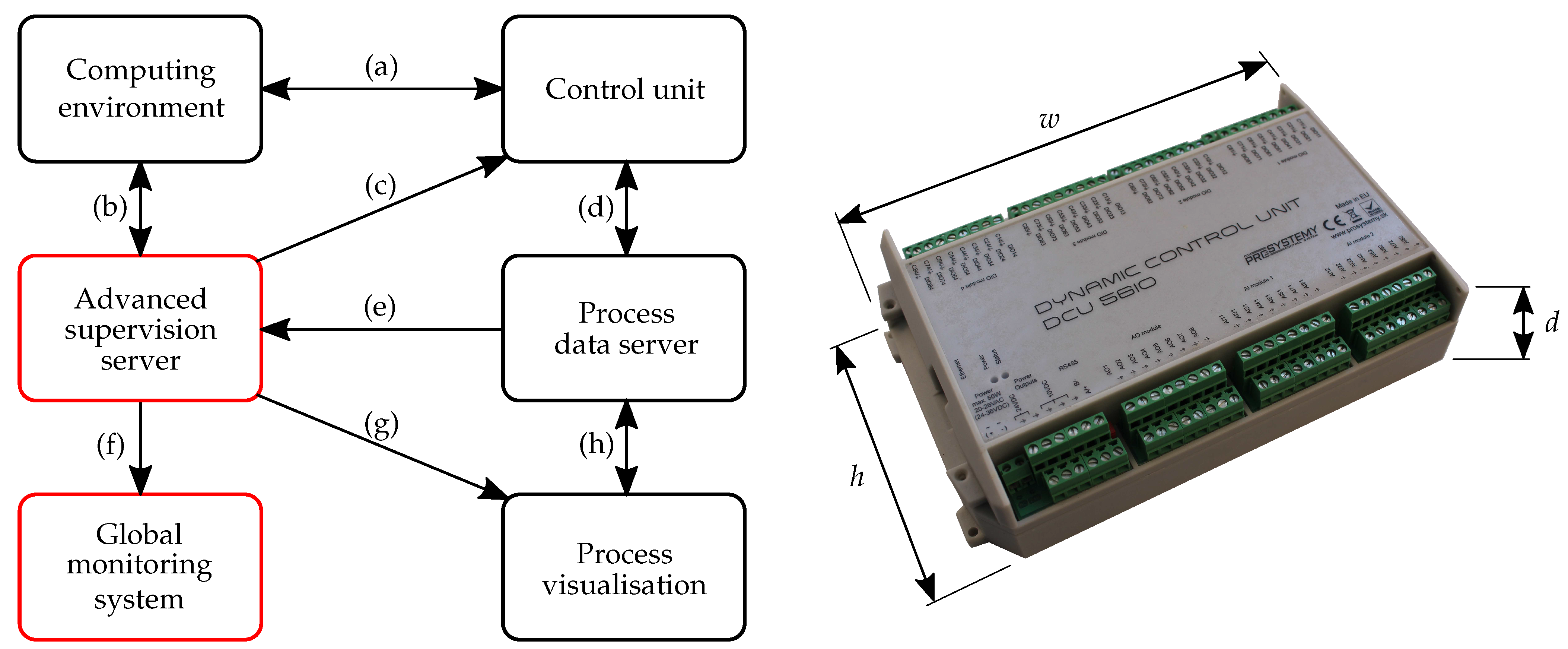
A simplified structure of the GMCS platform is depicted in Figure 1. The six main building blocks of the platform are divided into three layers. The arrows between the blocks illustrate one-way and two-way communication channels, labelled by (a)–(h) letters. The highest layer represents control design and real-time control. For control design and programming MATLAB/Simulink or its alternative Scilab/Xcos are used—Computer Environment (CE). The latter open-source alternative is however preferred as it can be freely distributed. TCP/IP communication protocol (a) is used for uploading a control application diagram from the host PC to the DCU control unit and UDP/IP protocol for communication between control units. The process data are collected in real time by the DCU. Process Data Server (PDS) PC receives the data from DCU (d) and records them into MySQL database. ASServer represents a package of advanced online procedures executed in the background. The advanced procedures uses relevant data from PDS (e) to analyse them in terms of fault, peaks and outliers detection, frequency and time domain analysis, process modelling and identification, online controller tuning, etc. The computing environment is used to evaluate these operations, thus mutual communication is integrated (b). The obtained results may by transmitted directly to DCU (c) or they can be presented to the process operator (g). Global Monitoring System (GMS) and Process Visualization (PV) are included in the third layer of the GMCS. These elements represent HMI for monitoring and management of the process and its control. Together with ASServer and PSD, they represent advanced SCADA system of the GMCS platform. GMS and PV interfaces provide information, notifications, alarms, display current and historical data to the user or administrator via a Graphical User Interface (GUI)—web pages. This GUI conveniently presents process data and its dynamical behaviour, and also allows for an intuitive management of the system. In cooperation with ASServer (f), GMS creates a possibility to monitor and debug more complex processes or several systems simultaneously via a single interface.
The ASServer and GMS (highlighted in red in Figure 1) upgrade the standard structure (depicted in black in the same figure) of the control system platform to a new level, providing novel advanced and smart features. One such a feature of the ASServer is a function implementing the identification procedure presented in the next subsection.
To make the GMCS description complete, let us briefly describe the DCU control unit, while more details can be found in [7] or in technical specifications on the manufacturer’s websites [25]. In the context of this work, it should be noted that the GMCS platform is built on DCU. It is a universal, freely programmable, hard real-time control unit. DCU is able to operate as a standalone control unit, but it is necessary to take advantage of all features of the GMCS platform server PC (can be any low-cost mini PC). As a communication standard, Local Area Network (LAN), Wide Area Network (WAN) and in some cases also the standard industrial network (Modbus RTU) are utilised. Two types of DCU controllers are available. They differ in size and also in number of input/output (I/O) channels. DCU28IO has 28 and DCU56IO has 56 I/O channels, which are configurable just in the latter case. Each DCU has integrated power supply connectors, RJ45 connector (for UDP/TCP/IP communication), RS485 serial communication connectors for Modbus RTU industrial bus. The actual DCU56IO control unit is also shown in Figure 1.
An important role in providing advanced features into the GMCS platform plays the ASServer by online integration of specific function packages. These can be classified as follows: (1) Process variables analysis, including functions for analysing a specific I/O port, e.g., detection of anomalies, undesirable oscillations, etc. Our recent contribution in this context can be found in [7]. (2) DCU process dynamics and control analysis, including functions for process identification, advanced control, etc. The procedure proposed in this study belongs to the second class of functions. These functions operate in background of the control system and administrator or operator of the process only needs to define several parameters required for the specific function.
2.2. Data-Driven Identification Function
This section presents a fully autonomous procedure for linear data-driven online identification. This procedure is developed in the open-source programming package Scilab and integrated into GMCS open-source control platform. The developed identification function, designated as processIdent(), belongs to the second group of ASServer functions dedicated to process control analysis. The procedure employs black-box modelling and parameter identification of a linear mathematical model in ARX (Auto-Regressive with eXternal input) and ARMAX (Auto-Regressive Moving Average with eXternal input) form. The identification procedure also integrates appropriate data pre-processing performed within specific time frames of the input–output process data. Based on informativeness of the data sets, several model structures are identified, validated and compared. The best model is then selected and compared with the previously identified model.
According to [6], three basic entities are involved in the modelling procedure: (1) the data record, (2) the set of candidate models or the model structure, and (3) a rule utilised for the assessment of model quality. After that, the model validation shall be performed in order to test suitability of the model for its purpose. There are several structures of the transfer function models, from which the most common in signal processing applications, ARX and ARMAX, are used. The ARX model represents the simplest input–output relationship. It is defined by linear difference equation incorporating the stimulus signal. The AR refers to the autoregressive part and X to the extra input (exogenous variable). Within the AR part linear regression equation is solved analytically, thus the model estimation is very effective. On the other hand, the stochastic dynamics (disturbances) are involved as a part of the system dynamics, affecting the estimation of the ARX model. Note that in order to minimise the equation error the model order can be increased. In that case it is necessary to take into account the possibility of distorting the dynamic properties of the model. In case of ARMAX model, the disturbances are included in the model structure, thus in comparison with ARX, ARMAX enables more flexibility by defining the error equation as a moving average of white noise (the MA part). This type of structure is suitable if the modelled system has dominating stochastic dynamics already present at the beginning of the measured process.
Along with the ARMAX and ARX parameter estimation functions, several other macros are utilised in the identification procedure. These functions are implemented in the Identification Toolbox for Scilab 5.4.x designed at the Department of Control Engineering, CTU Prague, by M. Novotny and A. Cornet [26]. Our procedure processIdent() is partly relies on this tool. However, before describing the identification itself, we shall chronologically introduce the essential parts of the code of the proposed procedure.
First, several variables have to be defined by the operator via PV or GMS interface. Values of these variables relate to the specific process to be identified, namely the minimum signal length in seconds and maximum model order. At the beginning of the processIdent() function, five more variables are defined, which are not accessed by regular user, but the administrator. Three of them are number of resulting elements (matrices), minimum distance of zeros and poles, and variable enhancement, which is a limit to determine model enhancement with order of the system. The other two indicate whether the function is to be performed in normal, graphical or debugging mode, or in debugging and graphical mode simultaneously. Normal mode means that only the result of the procedure and a notification of successful/unsuccessful function execution are provided to the operator.
After definition of these variables via GMCS, processIdent() function is set to evaluate the measured data. The process data are provided by PSD in a data file form, which together with input/output time data includes several other information. Enabled/disabled information (signal with the same size as input and output data matrix with 1 or 0 value indicating enable or disable identification procedure, respectively) and those listed below in Listing 1. The structure of the input data file is the same as in case of the structure used in [7], making this concept uniform.

Listing 1.
Structure of the input data file.
| Row 1—name of output folder path and file where to store results. Row 2—informative message or any optional string. Row 3—number of input parameters (matrices) for identification. Row 4—number of results (if previous results from analysis need to be considered). * Row 5—definition of matrix dimensions (number of rows and columns). Row 6—the first row of matrix (timestamp and value of measurement). Row 7..(x − 1)—other rows of matrix (each row is on new line—new measurement). † Row x—number of initial parameters or previous results respectively. Row (x + 1)..(x + y)—matrix dimensions and rows values—analogous to part between * and †. |
Unix timestamp is a sequence of characters representing date and time in seconds that have elapsed since the Unix epoch. The Unix epoch is 00:00:00 UTC on 1 January 1970.
As it is a universal structure for the whole package of proposed and developed functions, the same rules apply in this case as well. Thus, each signal (input, output and activation) is written to the input file between * and †, as specified in Listing 1. The last lines of the input document list the initial polynomials of the ARX or ARMAX model. If polynomials from a previously identified model are available, the best ones are written here. An example of an input data type can be found in Appendix A, in which input, output and enable signals have 1000 samples (the first and last three measured data are displayed) and the previously identified model is described by the displayed polynomials.
The input data file is read by the processIdent() function in user-defined schedule or pre-set time periods, therefore data from the actual time window are available. They are then subject to preprocessing necessary for further evaluation of the procedure. The complete evaluation procedure consists of the following five steps:
- At first the process input/output and enable/disable signals are withdrawn from the input data file, after which their synchronisation in terms of start time is performed. Only data from a measurement in which the enabled signal has a value of logical 1 are taken into account in the identification. Subsequently, each of three signals is processed separately. Within this preprocessing embedded function a sampling time of the signal in seconds, signal duration and segmented time, as well as amplitude vector of the signal are determined. Their segmentation is evaluated based on a data continuity check and NaN samples finding. In case there are omitted samples in measurements, the function handles this by interpolating the values or by breaking the signal into two segments at that sample. For more information see [7] where the same approach was used.
- Next, the procedure continues by evaluating the number of their segments and searching for their data overlap. Each signal is truncated according to the manner the intersections of the segments were determined. In consequence, the requirement defined by operator—minimum length of signal segments to be identified—is checked. If there are suitable signal segments, the function processIdent() in the graphical mode shows them in a graphical window.
- Once the pre-processing is finished the system identification is performed. We remark that only the first Ljung’s modelling entity has been implemented by this point and the second and third point still need to be evaluated. The above mentioned Identification Toolbox is used to address these two stages. Specifically, to create the model structure idmodel() function is used, which is contained in armax() as well as arx() function of this toolbox. The armax() and arx() functions are used for estimation of model parameters based on input–output data by recursive least squares method—third Ljung’s modelling entity.
- After parameter estimation, the model is validated by fit_model() function which computes Mean Square Sum Error (MSSE), being the mean of squared differences between measured and simulated output. This sequence of estimation and model validation is evaluated in cycle in as many times as is the maximum model order set by the operator. Yet, if there is no improvement in model with higher order in comparison with previous one, the cycle is terminated. Improvement of the model is based on comparing MSSE of the last estimated model with the best one so far. In addition, the distance between the poles and zeros of the model polynomials is compared in order to avoid the model to be over-ordered. The same procedure is evaluated for both ARMAX and ARX modelling methods. The decision on the best model found is made afterwards, and the best model is selected based on the minimal MSSE of the particular model with data in all signal segments. If there is a previously identified model available in the input data file, this model is also validated with new data and compared with newly estimated model. If there is an improvement, the new model is written to the output data file as a result and thus it is also taken as a model for comparison in further function evaluation. In case of graphical mode, the graphical output is provided to operator.
- Finally, the result is written to the output data file created with the path and saved with the name defined in the input data file. The structure of the output data file is presented in Listing 2. The status of the procedure evaluation is also available to the user in GMS or PV, respectively, where it is loaded from the generated output data file. Note that the above identification procedure can be used as a basis for online tuning of the PID controller or other advanced control functions.
Listing 2.
Structure of the output data file.
| Row 1—return message for user (status of the procedure evaluation). Row 2—the best attained fit by the procedure. Row 3—value of model improvement rate. Row 4—new model polynomials if better have been found. |
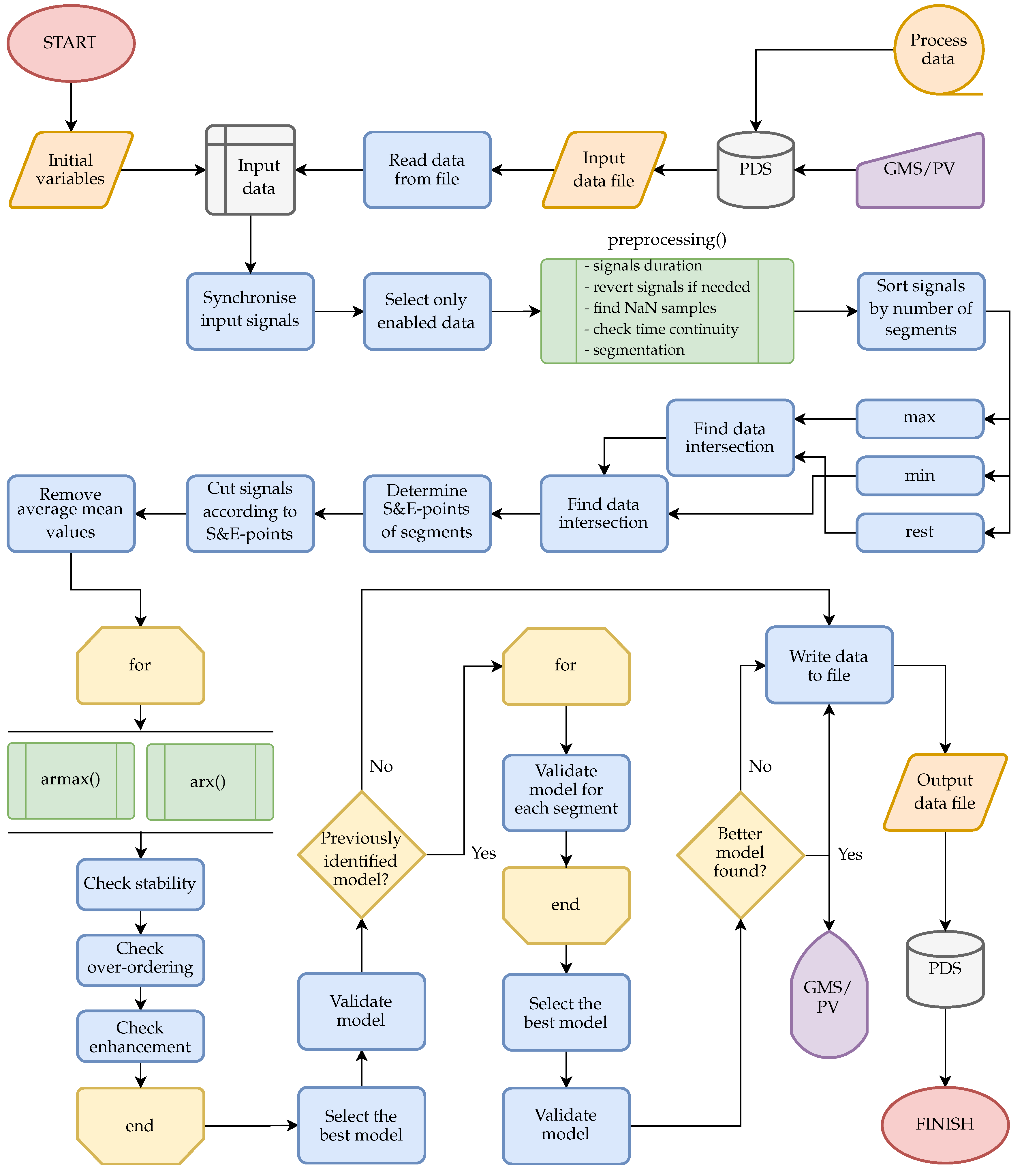
To make the procedure of the processIdent() function more understandable for the reader, it is illustrated as a flowchart in Figure 2. There are three main subroutines—namely preprocessing(), armax() and arx()—which are depicted by green blocks. There are also several auxiliary other functions from the Identification Toolbox [26] used for parameter estimation that are included in armax() and arx() subroutine blocks in the flowchart. Next, our readMatrices() function is used to read data from input matrices and this is hidden under the ‘Read data from file’ block. Each action in the procedure is represented by the blue block. The yellow blocks represent built-in loops and decisions, orange and grey blocks in turn data sources and storages. Finally, the HMI in terms of manually defining input data and reading the procedure output in the visualisation environment is depicted in purple colour.
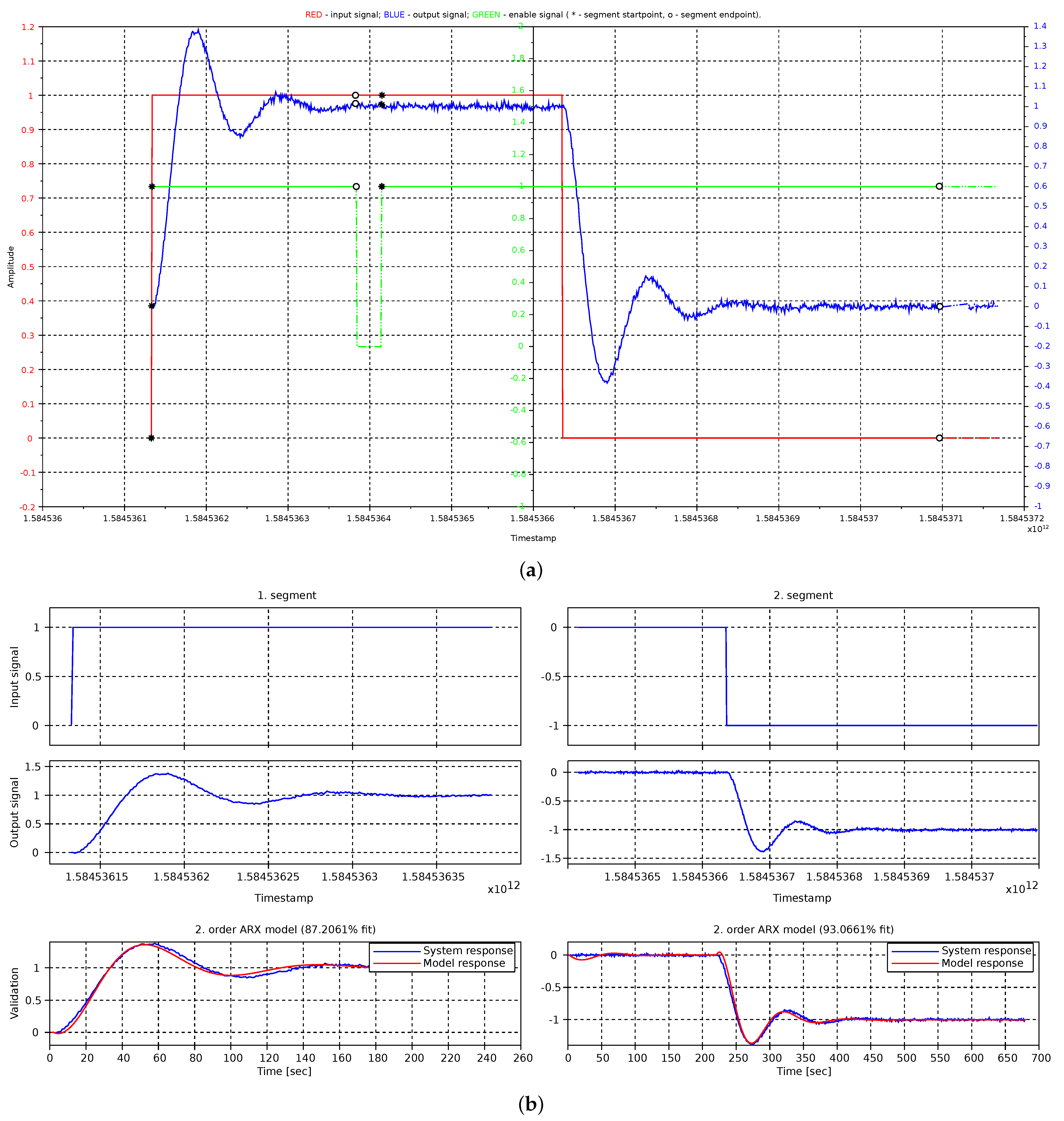
In order to validate the functionality of the proposed identification procedure, several offline simulations were performed. One of them is captured in Figure 3. Within this experiment, the process data were obtained from simulation in Simulink, where a simple input signal was applied to a second-order system and white noise was added to output data. Enable/disable signal was set to value 1, thus identification was enabled all the time except a 30-s long time window, where the value was set to 0 (see Figure 3a). Input data file (see Appendix A—Input) was also created off-line and subsequently used as an input to the processIdent() function. Graphical output from simulation of identification procedure can be seen in Figure 3b. It can be seen in Figure 3 as well as in the console list included in Appendix B that the signals were divided into several segments and afterwards two suitable segments were determined. Input, output and enable/disable signals are plotted by solid line within these segments. Signals which do not meet all requirements for further identification procedure are plotted by dash-dotted line. Start-points and end-points of the segments are highlighted by ‘*’ and ‘o’ marks. Consequently, the identification procedure was performed for each segment separately. Validated models are compared with system responses in the third row of graphs in Figure 3b. A numerical value of fit is written into the titles of these graphs. It should be noted that this percentage value represents the fit factor between measured and validated data according to the fitFactor() function from the dedicated Scilab toolbox (see in [26]). More information on the procedure sequence can be found in Appendix B.
The proposed procedure is experimentally tested in the laboratory as well as in the real-world environment by means of a unique laboratory HVAC system for software development and a two storey house to validate the functionality in practice. We describe this in the following section.
2.3. Laboratory HVAC System and Residential House
It is very beneficial not only from the practical point of view, but also due to time and cost effectiveness, to use an adequate physical model which could be used as a mean to simulate, develop and improve identification and control algorithms (such as e.g., in [27,28]). For this purpose we used our case study equipment—a laboratory HVAC system. This testbed has been constructed recently, designed mainly for experimental validation and verification of novel control techniques using the DCU control platform. The testbed has been introduced in [24], where we discussed experimental testing of a signal analysis function. In another work [7], a real two-storey house was used for practical testing. In this study, both of these testbed environments are used, hence their specification and functionality description are needed first.
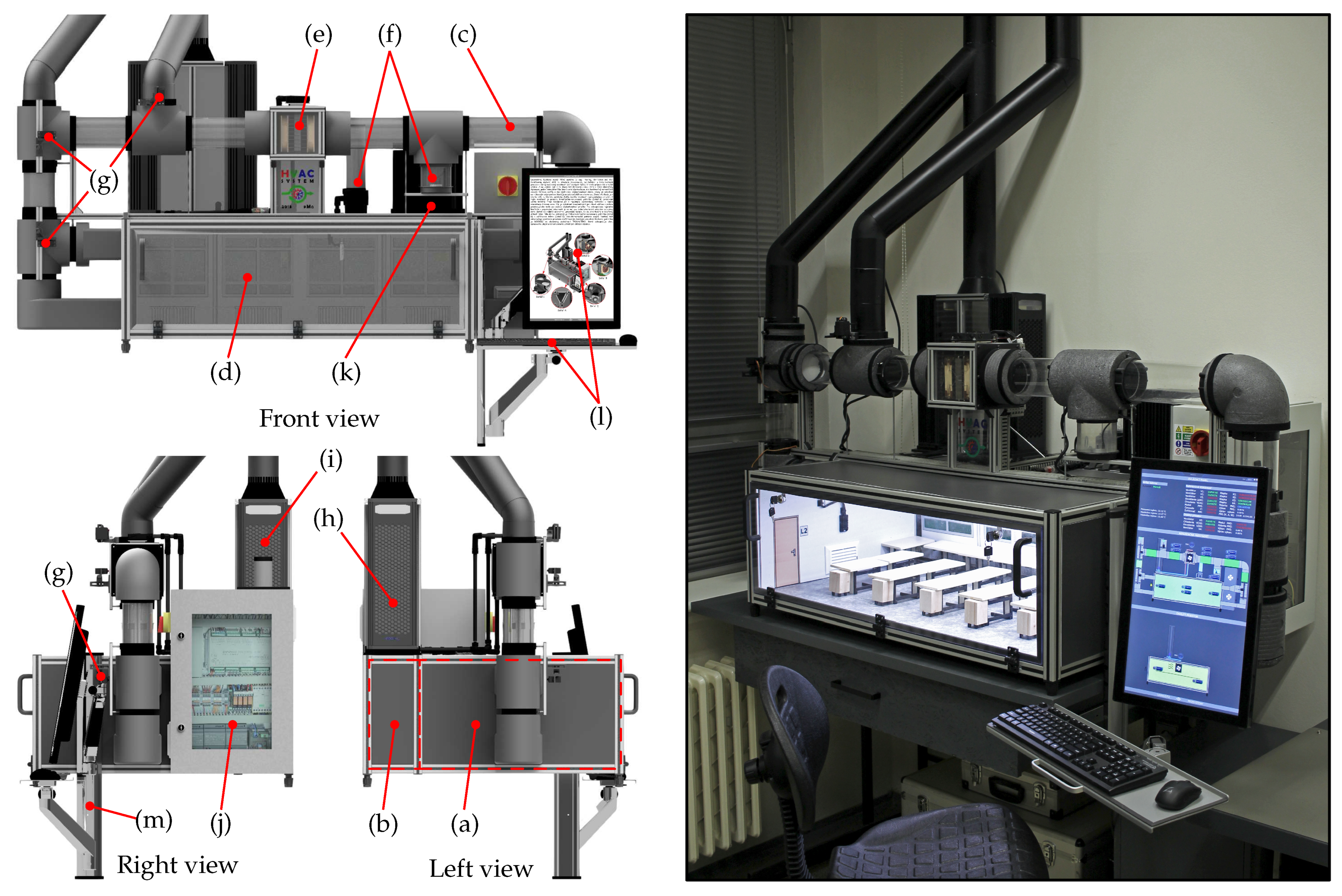
The design of the laboratory device was based on several main features: (1) It shall consist of at least two rooms, one representing interior served by a heating, ventilation and air-conditioning circuit and disturbed by the second room representing thermal conditions in exterior. (2) There shall be at least two process variables—air temperature and relative humidity generated by an appropriate heating/cooling unit and humidifying device. (3) It shall integrate a suitable HMI to control and monitor processes in the testbed. (4) It shall have a minimalist but innovative hardware design. Coming from these basic, but also other non-negligible physical model requirements, a laboratory system was created in the form as shown in Figure 4.
The left-hand side of Figure 4 also shows three views of its CAD model, where letters denote particular parts of the laboratory HVAC system. Its construction has three fundamental parts—the reference room (room-1) labelled as (a), the neighbouring room-2 (b) located behind room-1, and (c) air ducts attached to the room-1. The room-1 is conceptually designed as a room that is in contact with the exterior by means of only one wall, such as most rooms in office buildings or semi-detached houses. Specifically, inner dimensions of the room-1 are scaled in 1:10 ratio to a real classroom at the authors’ workplace, which also interacts with the exterior with only one wall along one side. Thermal comfort conditions are desired to be achieved in this space, the volume of which is approximately , while in room-2 with cca. quarter of the specified volume pseudo-random thermal disturbances are generated to affect room-1 through the dividing wall.
The air ducts contain sensors and actuators including a heating–cooling unit (HCU-1) in Figure 4 labelled as (e), a humidifier (f) and air dampers operated by servomechanisms (g) ensuring air flow to/from one of the two inlets/outlets and to/from the exterior. Positioning of the air dampers depends on one of three operating modes of the HVAC system. It was designed to operate in heating, cooling and ventilation mode, derived from the three essential HVAC processes in general. To increase and decrease air temperature in room-1 the HCU-1 is used. It contains a thermoelectric module and a radiator with fans. Note that the heating and cooling modes depend on electric power polarity of the module, therefore a cooler for the outer side of the module is needed as well (h). The same configuration is used in room-2, but HCU-2 is immersed directly into room-2 instead of air ducts. The cooler for the HCU-2 (i) is situated next to the cooler for HCU-1. Since the value of relative humidity of the air is also controlled in room-1, an ultrasonic humidifier with water reservoir serves to increase it. Among other, but not less important parts of the laboratory model is an electronic box (j), which accommodates all necessary electronic components and the DCU56IO control unit. From this box, all actuators, lighting, water pumps, air fans and sensors in the testbed are powered. In addition, an industrial PC (k) and touch-screen monitor with PC peripherals (l) serve as HMI for the user to monitor and control ongoing processes in the HVAC system. For more details on this unique testbed we refer the reader to [24].
As it has been stated above, the laboratory model works in three modes—heating, cooling and ventilation. Let us briefly describe these operating modes and functionality of the model. In order to introduce an appropriate terminology, in Table 2 we first define different types of air present in the HVAC system.
Each of aforementioned operating modes is based on air circulation from HCU-1 through ducts into the room-1, where an ‘X-logic’ of air flow is ensured by air dampers and two inputs and outputs in order to provide the most possible thermodynamic exchange between the supplied air and the air in room-1. Air dampers direct the air flow to one of the two input air openings situated at ceiling level and at floor level of the room-1, while on the opposite wall of room-1, one of the two output air openings is used to extract the exhaust air. Not only the air passes along this diagonal trajectory, it also encounters obstacles in the room, causing a turbulent flow. Which openings are used depends on the current operating mode.
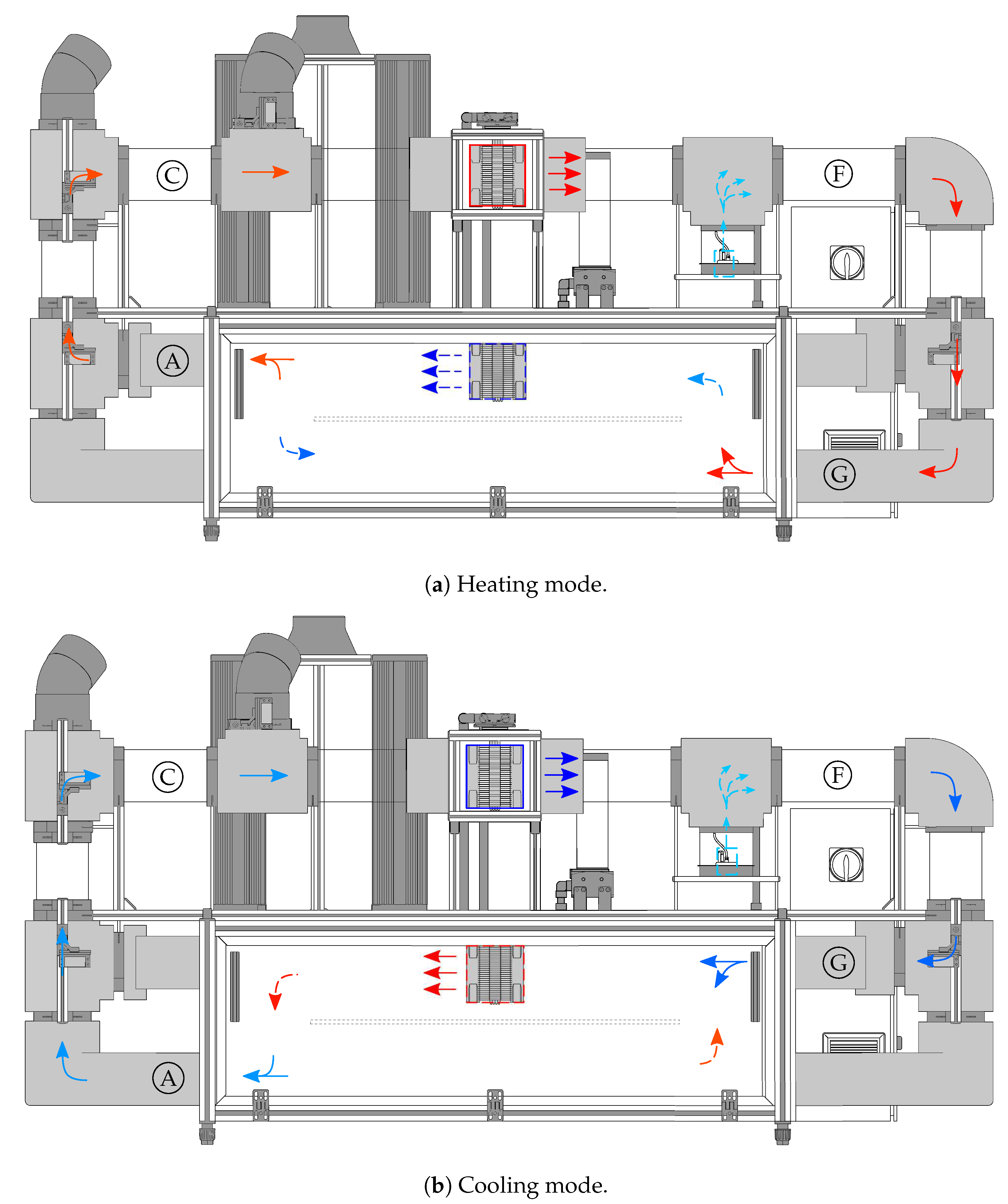
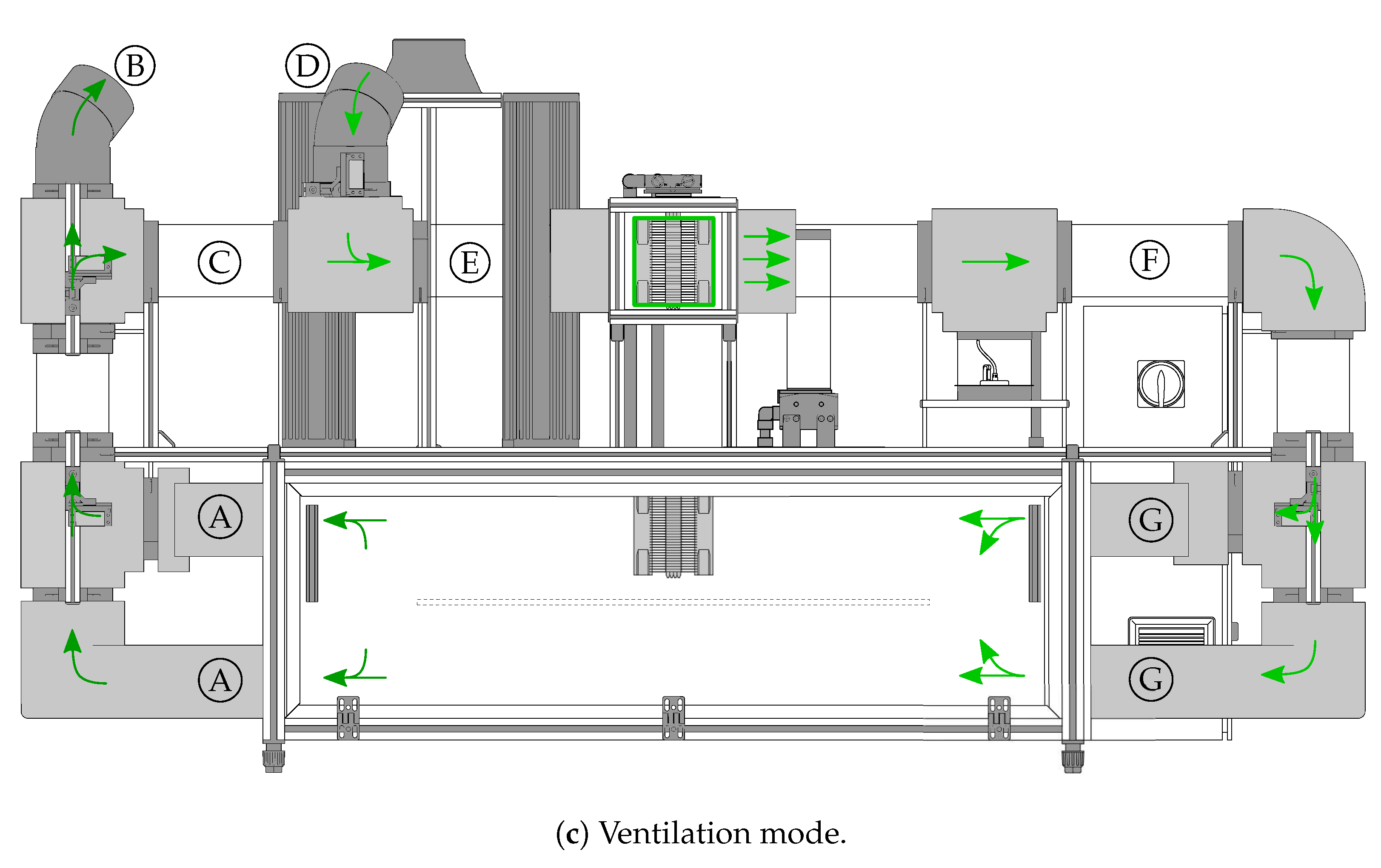
For a better understanding we attach illustrative diagrams in Figure 5. As shown, air from room-1 is exhausted through the ceiling level opening, then it passes through HCU-1 and humidifier. After that, conditioned air is blown by the fans into room-1 as supplied air through floor level opening in heating mode. In Figure 5a this circulation is denoted by red arrows, while light blue colour represents the air humidification process and dark blue arrows represents air flow direction in room-2. Therein thermal disturbances in form of cold air are generated simultaneously by HCU-2 (dark blue arrows in Figure 5b). This represents HVAC system simulations in winter season or during day/night service. On the contrary, hot air is generated in room-2 at the same time when the system is in cooling mode. The opposite situation is also in the case of room-1, where the air is exhausted from through the floor level opening conditioned by HCU-1, and supplied air flows through the ceiling level opening into room-1. This is illustrated by dark blue arrows in Figure 5b. Note that in the cooling and heating mode fresh air can be also aspirated to the system from the outdoor environment by air damper and subsequently outside air is mixed with returned air and forced to further thermodynamic treatment. Similar situation can be seen in ventilation mode illustrated in Figure 5c, where it is required to bring the fresh outside air into room-1 through arbitrary input openings and through arbitrary output openings it is exhausted to the exterior as a relief air. In ventilation mode, the HCUs work merely as an air propulsion equipment since only their fans are used.
As already outlined, two observed quantities are monitored and controlled, while their physical properties are conditioned by HCU-1 and humidifier. In this study, several signals were selected as a parameter for processing by the designed identification function described in Section 2.2. For the purpose of its real-world validation, an experimental two-storey family house has been used. This family house situated in Bratislava, Slovakia, has a basement with sauna, indoor pool, cellars and a technical room. The technical room is equipped by the control and computing technology, including electrical wiring, storage tanks, pumps, heating exchanger, etc. Together with this equipment, six DCU56IO control units are situated in central electrical box serving another two floors above the ground with six rooms. It is therefore a quite complex system involving several technologies to be controlled. The Prosystemy company has this residential building at disposal for experimental verification of the developed procedures.
3. Results
This section presents the experimental results obtained in testing of the proposed online data-driven identification procedure using the described testbeds.
3.1. Experimental Setup
Room-1 of the laboratory HVAC system was selected for experimental verification. Specifically, it is a filtered temperature signal in from only one sensor located behind HCU-1, i.e., the first sensor in the air duct in terms of air flow direction. Process data from cooling and heating operating modes were used, so two graphical outputs from the identification procedure are included (see Figure 6 and Figure 7). These are three-hour experiments in which the input value being the electrical power to the Peltier module in 0% to 100%—was changed five times.
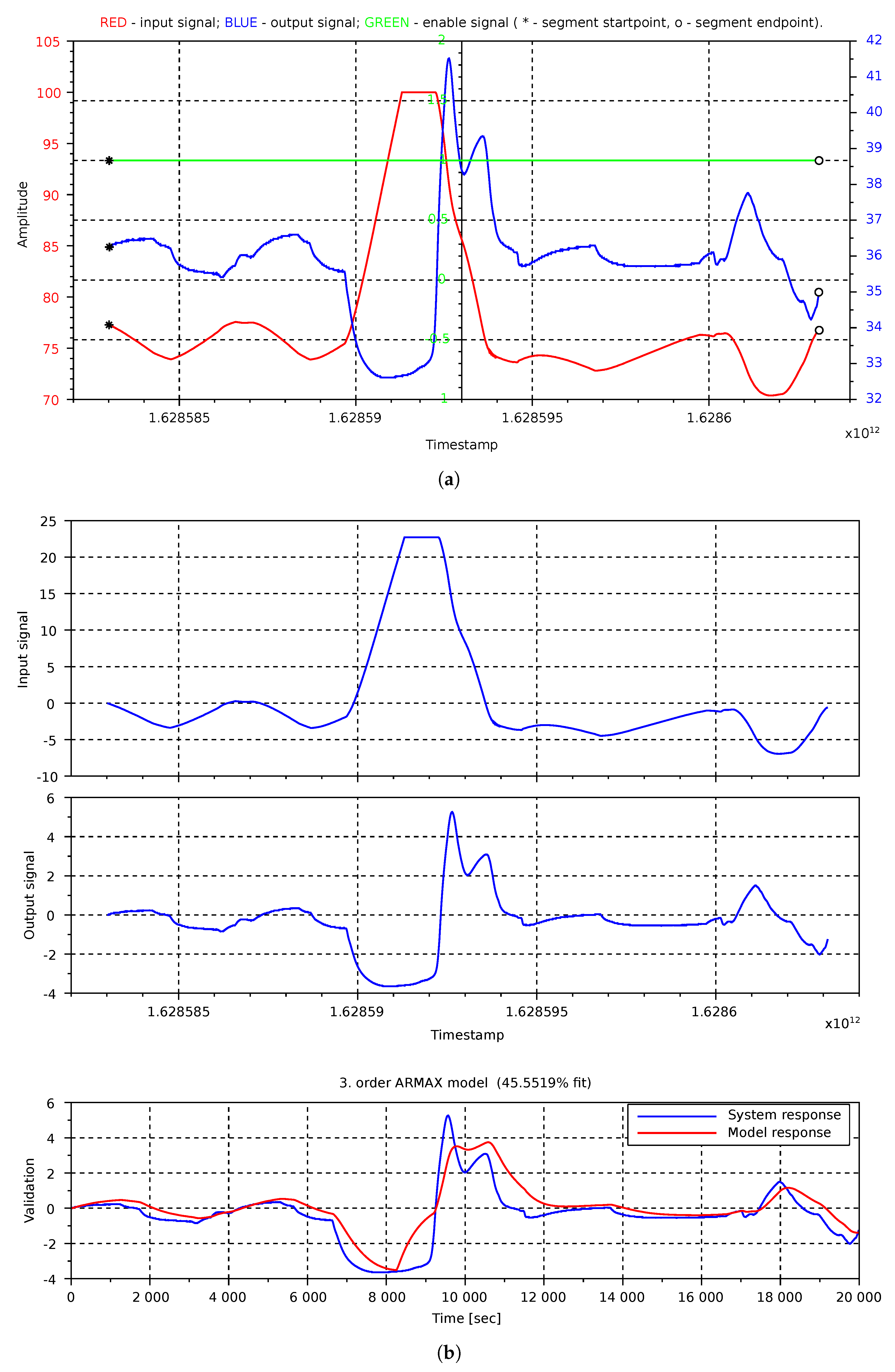
In case of experiments carried out in the real building, one input and one output signal were also selected for identification. The water temperature in at the beginning of the underfloor heating system in the basement of the house was chosen as the process output and the valve opening position in the range of 0% to 100% (0%—closed and 100%—fully opened) of a three-way valve ensuring hot water supply from the boiler as an input signal. The identification data were selected from a time frame of approximately six hours. The respective graphical outputs are shown in Figure 8 and Figure 9.
Since the concept is uniform, input and output data file structure are the same in all advanced functions (see also [7])). Some information required for the identification process are provided via a process visualisation interface as well. This interface is available on any device with an installed web browser, so setting up an identification process is very simple for the operator.The input, output and enable signals are defined in the visualisation environment. An example of the entire list of setting parameters can be found in Table 3. In this example, the data-driven identification will be performed every four hours for six-hour signals. The minimum signal segment length is set to ten minutes. The maximum order of the model is set to 5 and the initial polynomials of the model are not set, hence zero values are set. The same parameters were set in the performed experiments, except for the minimum signal length, which was set to 50 . Duration of the identified signal in the laboratory HVAC system experiment was different too, being .
3.2. Experimental Results and Discussion
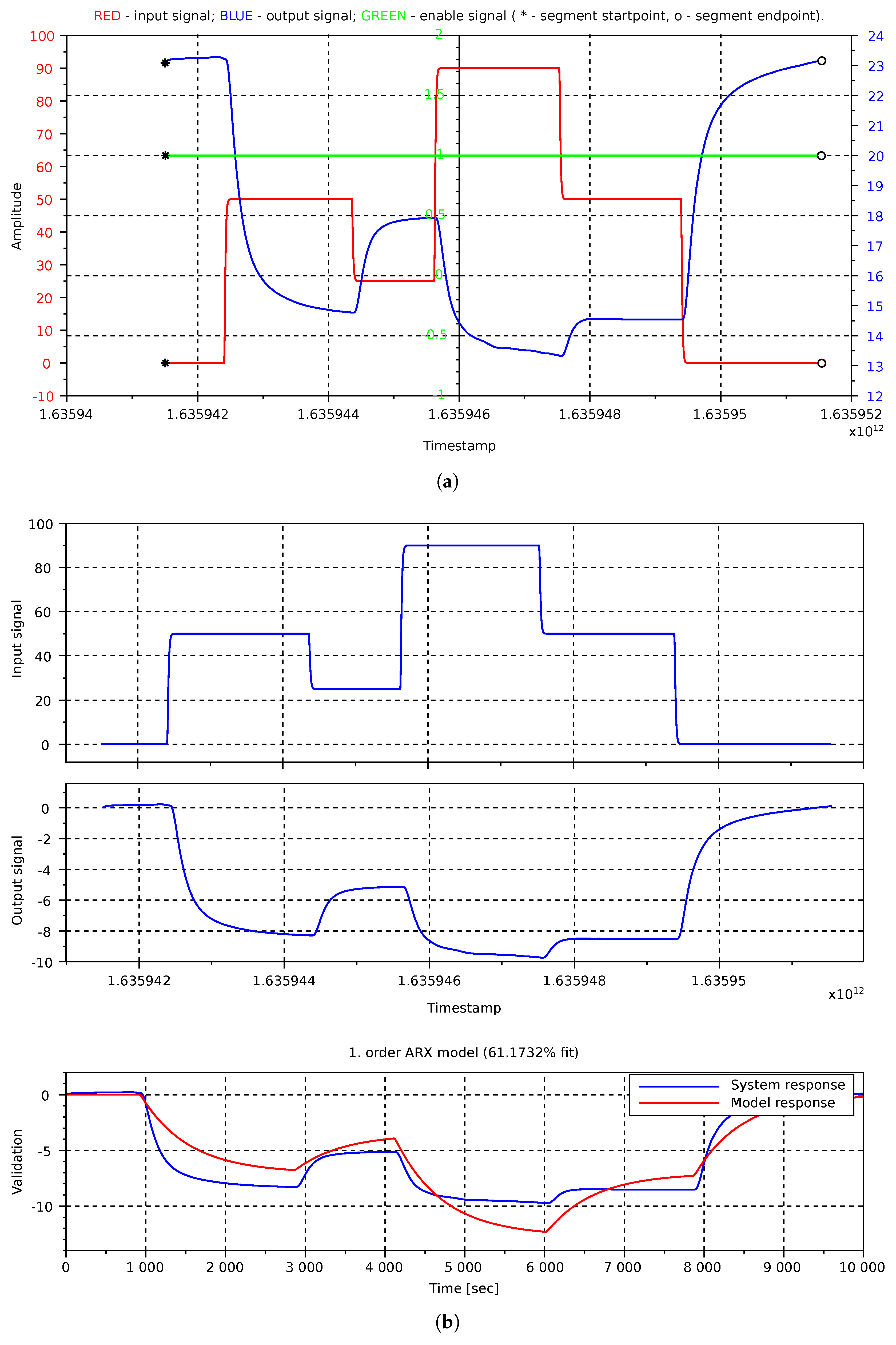
Air temperature signal evaluation in cooling mode of room-1 is captured in Figure 6a in blue colour. The red line represents input signal moving in four levels of input electrical power to the Peltier module. The first change occurred to 50%, then it was halved, and subsequently increased to 90%. Finally, declined to half power and then to zero. It can be seen from the graph that the output signal reacted rather quick to this input what is caused by a shorter distance between actuator and sensor. The enable/disable signal was set to value 1 at all time, so the identification process was enabled throughout the entire experiment. In addition, no signal outages occurred, thus a complete data set was measured. Hence, signal segmentation was not needed and the signals measured within this experiment were identified as one segment in one iteration. Input and output signals used for identification are depicted in the first and the second graphs in Figure 6b. There you may notice that the medium average values from the signals were removed due to a better result of identification process. Within the identification procedure, a first-order ARX model was identified; see also Table 4. The third graph shows validation of this model. The graphical comparison of the model response (red line) with the system response (blue line) is captured here. Not the best model fit (61.17%) was reached in this case, which is mainly caused by an insufficient excitation of the system.
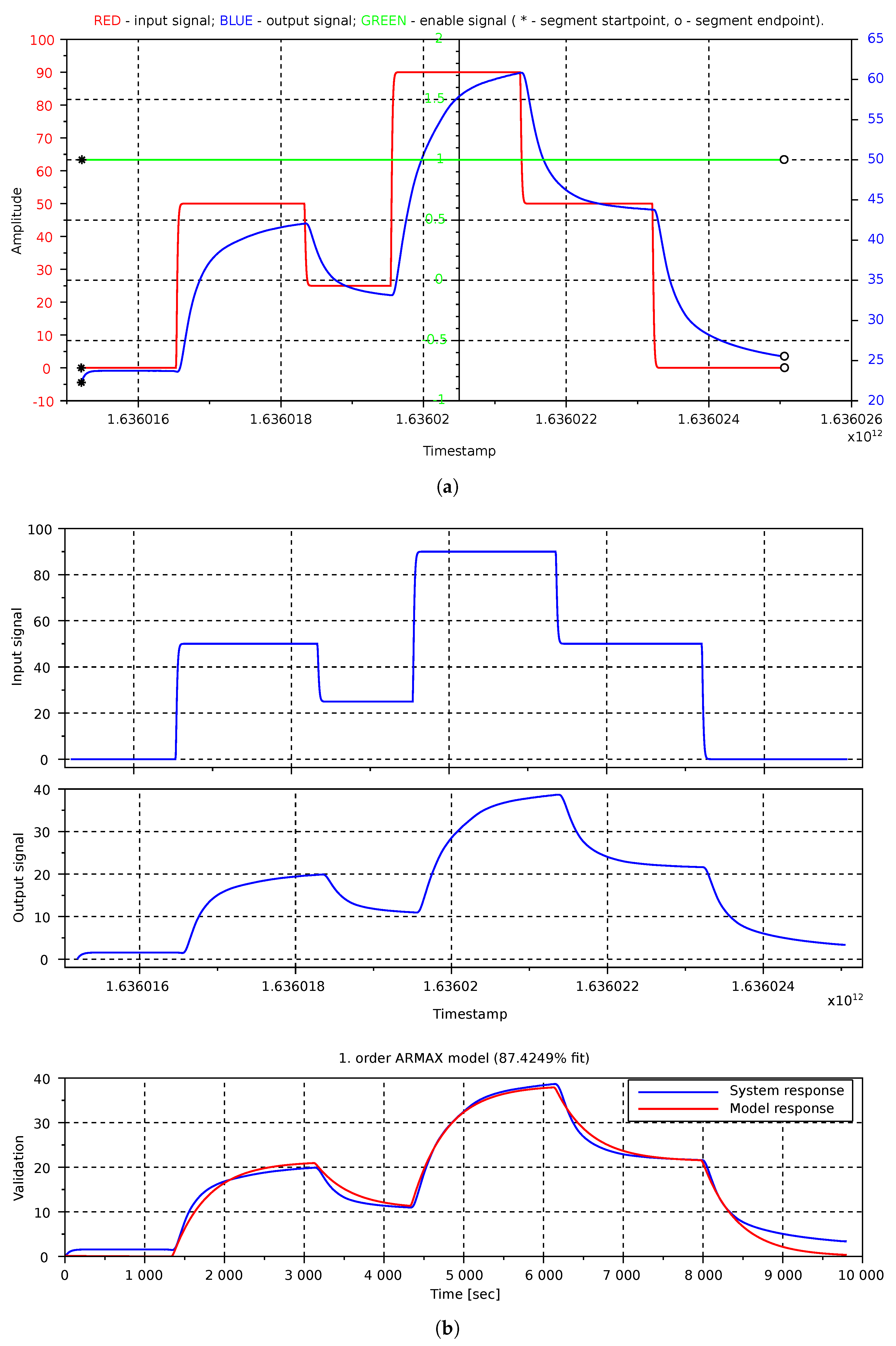
On the other hand, heating mode of the same room was identified satisfactorily. The experimental conditions were almost the same as in the previous case of cooling mode. The input and output signals were evaluated as one segment as well (see ‘*’-sign and ‘o’-signs in Figure 7a). Thus, the identification was enabled all the time during the experiment and there were no signal anomalies. The input signal was also designed likewise. More specifically, after about 20 the input electric power for Peltier module in HCU-1 was set to 50% at which it was held for 30 . After that the input power reduction to 25% for 20 was performed and consequently increased up to 90%, where it was kept for another 30 . Finally, the input signal was decreased to 50% and after another 30 the Peltier module was turned off. While the values are read from the same sensor as in the previous experiment, the response to the input signal is fast as well. Together with the process input and output signals with the mean values removed, there is a graphical comparison of the identified first-order ARMAX model (see Table 4) response and the system response shown in Figure 7b.
After testing the functionality of the data-driven identification procedure in laboratory conditions with satisfactory results, it was possible to design and perform an experiment in real operation of the HVAC system within the two-storey house. Two of all performed experiments are presented next. In both of them the enable/disable signal was set to the value of 1. In the first experiment, the input and output signals did not show any discontinuance, so they were considered as one segment in identification process (see Figure 8a—red and blue lines). The experiment lasted about , while the input signal—valve opening rate—varied between 70% to 100%. Depending on that, the temperature of water flowing to underfloor heating system reached values between about 33–41. These signals with removed mean values are captured in the first two graphs in Figure 8b. The best found model fit the system response in 45.55% and its validation graphical output is depicted in the third graph of Figure 8b. As shown in Table 4 a third-order ARMAX model was identified. The percentage indicator is low, but according to the graphical validation output it is a satisfactory result.
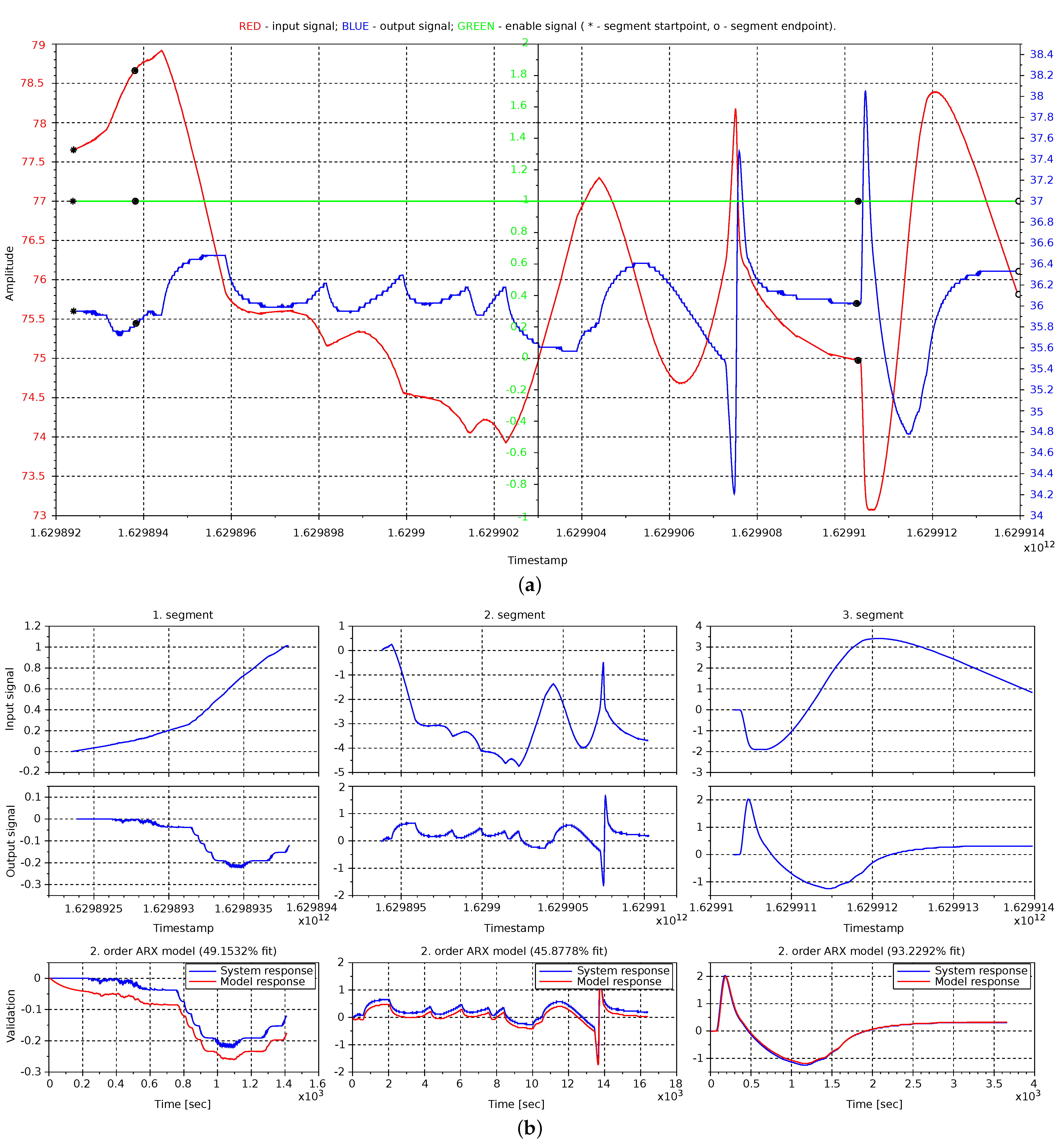
A better situation can be seen in the experiment with graphical output depicted in Figure 9. In this case the signals were divided into three segments, although the enable/disable signal was set to value 1 during the entire experiment. This was caused by signals discontinuity in terms of time sequence, leading to a number of missing measurements following each other or the NaN (Not A Number). The start and end of segments are highlighted by ‘*’ and ‘o’-signs (see Figure 9a). Hence, the further identification process was divided into three parts, i.e., each segment was identified separately. Similarly to previous examples, the input and output signals in each segment together with validation output are shown in Figure 9b. In the titles of validation graphs one can inspect the numerical value of fit, being 49.15%, =45.88% and 93.23% fits, while in all cases a second-order ARX model was evaluated as the best. However, the best model overall needs to be found, thus a validation of these models is performed for two other segments as well. The model with minimal deviation with respect to system response in sum for each segment is considered as the best model. For more information see Table 4 which lists the numerical results obtained these experiments.
In summary, the performed simulations and experiments demonstrate the functionality of the proposed linear process identification procedure as a part of another functionality emerged from our advanced control platform integrated in the open-source and universal control platform DCU. As a part of our future work we will focus on possible improvement of the presented approach which can further benefit from long-term deployments and tuning. While the procedure is easy to initialise (Table 3), there is a possibility of direct implementation in practice within offline deployment (on operator’s request) and thus to gain additional important knowledge and suggestions for improvement of this procedure based on experimental results.
4. Conclusions
In this study, we introduced a novel online data-driven identification procedure implemented within an advanced process supervision concept referred to as ASServer, integrated into the open-source and universal control platform DCU. Its functionality has been verified in offline simulations. We have demonstrated the implementation and experimental validation of the proposed identification procedure in the laboratory setting and in the real-world environment as well. As a case study, a laboratory model of HVAC system and a two-storey house were considered. The presented linear identification approach uses ARX and ARMAX modelling methods. The least-squares selection rule is used to assess candidate models. The identification is based on online data which are pre-processed and segmented eventually. Each segment is considered separately, so each has its own model, which is validated with process data from other segments. The most appropriate model overall is selected and utilised as a comparison model for the subsequent identification procedure. Based on the obtained results, we conclude that the proposed procedure as another GMCS software extension is fully functional. Its deployment in various experiments has proved a reliable service. The described function will be used as a basis for the design of other additional functions for process control as a part of our further work. Our goal is to build a complex open-source dynamic control system with the possibility of implementing advanced control techniques into common control engineering practice in the building, leisure as well as manufacturing sector.
Author Contributions
Conceptualization, P.M., H.P. and M.G.; methodology, P.M. and H.P.; software, P.M. and H.P.; validation, P.M.; formal analysis, P.M.; investigation, P.M. and H.P.; resources, P.M. and H.P.; data curation, P.M. and H.P.; writing—original draft preparation, P.M., H.P. and M.G.; writing—review and editing, P.M. and M.G.; visualisation, P.M.; supervision, P.M. and H.P.; project administration, P.M. and H.P; funding acquisition, M.G. All authors have read and agreed to the published version of the manuscript.
Funding
This research was funded by the Slovak Research and Development Agency under the grants APVV-18-0023 and APVV-20-0046. The APC was funded by the project ‘Predictive control of mechatronic systems and industrial processes’ under the programme ‘Excellent creative teams at Slovak University of Technology in Bratislava’.
Institutional Review Board Statement
Not applicable.
Informed Consent Statement
Not applicable.
Data Availability Statement
The data presented in this study are available on request from the corresponding author. The data are not publicly available due to privacy.
Acknowledgments
P.M. would like to thank for financial contribution from the STU Grant scheme for support of excellent teams of young researchers.
Conflicts of Interest
The authors declare no conflict of interest. The funders had no role in the design of the study; in the collection, analyses, or interpretation of data; in the writing of the manuscript, or in the decision to publish the results.
Appendix A. Input and Output Data File Example
- Input:
- C:/Users/minarcik/Desktop/processIdent/identOutput_2c.dat
- string
- 3
- 1
- 1000,2
- 1584536132898,0.000000
- 1584536133903,1.000000
- 1584536134907,1.000000
- 1584536135912,1.000000
- …
- 1584537164659,0.000000
- 1584537165664,0.000000
- 1584537166670,0.000000
- 1584537167675,0.000000
- 1000,2
- 1584536132898,0.003565
- 1584536133903,0.005111
- 1584536134907,-0.006437
- 1584536135912,0.001828
- …
- 1584537164659,0.001854
- 1584537165664,0.005423
- 1584537166670,0.007792
- 1584537167675,-0.001491
- 1000,2
- 1584536132898,1.000000
- 1584536133903,1.000000
- 1584536134907,1.000000
- 1584536135912,1.000000
- …
- 1584537164659,1.000000
- 1584537165664,1.000000
- 1584537166670,1.000000
- 1584537167675,1.000000
- Previous results
- 2
- 1,3
- 1,-1.486232,0.534421
- 1,3
- 0,-0.190926,0.239978
- Output:
- MESSAGE: OK: Identification done!;
- MATRIX_0: [91.3938];
- MATRIX_1: [1];
- MATRIX_2: [[1,-1.9517779,0.9565069][0,-0.0197048,0.0244584][0,0,0]];
Appendix B. Scilab Console List during the processIdent() Procedure
- –>processIdent(’identInput_2c.dat’)
- -> Reading data from file…
- OK: Data have been read from file.
- OK: Input data have been read.
- OK: Previous results have been read.
- -> Data preprocessing…
- OK: The signal is not continuous-time and has been divided into 2 segments.
- OK: A duration of the 1. segment is 964.623 [s], being more than 50 [s], so this segment will be considered in further procedure.
- WARNING: A duration of the 2. segment is 34.652 [s], being less than 50 [s], so this segment will not be considered in further procedure.
- OK: The signal is not continuous-time and has been divided into 4 segments.
- OK: A duration of the 1. segment is 249.522 [s], being more than 50 [s], so this segment will be considered in further procedure.
- WARNING: A duration of the 2. segment is Nan [s], being less than 50 [s], so this segment will not be considered in further procedure.
- OK: A duration of the 3. segment is 683.947 [s], being more than 50 [s], so this segment will be considered in further procedure.
- WARNING: A duration of the 4. segment is 34.652 [s], being less than 50 [s], so this segment will not be considered in further procedure.
- OK: Selected signals have same sample time and will be identified.
- OK: The maximum number of segments is 2.
- OK: The minimum number of segments is 1.
- OK: There are two minimum numbers of segments, which are equal to 1.
- -> Finding data intersection in segments…
- OK: Intersection 1-1 is long enough.
- OK: Intersection 1-2 is long enough.
- OK: Intersection 2-1 is long enough.
- OK: Intersection 2-2 is long enough.
- OK: The 1. segment of intersection has been found in the 1. segment of the 3. signal.
- WARNING: The 1. segment of intersection has not been found in the 2. segment of the 3. signal.
- WARNING: The 2. segment of intersection has not been found in the 1. segment of the 3. signal.
- OK: The 2. segment of intersection has been found in the 2. segment of the 3. signal.
- OK: Data preprocessing done!
- -> System identification…
- -> System identification of the segment 1:
- OK: ARMAX model for 1. segment has been identified with the 1. order and the fit is 0.0350957.
- OK: ARMAX model for 1. segment has been identified with the 2. order and the fit is 0.0307637.
- OK: ARMAX model for 1. segment has been identified with the 3. order and the fit is 0.0237152.
- OK: ARMAX model for 1. segment has been identified with the 4. order and the fit is 0.0191336.
- OK: ARMAX model for 1. segment has been identified with the 5. order and the fit is 0.0144833.
- OK: ARX model for 1. segment has been identified with the 1. order and the fit is 0.0495796.
- OK: ARX model for 1. segment has been identified with the 2. order and the fit is 0.0022246.
- WARNING: ARX model with the 3. order is for 1. segment unstable.
- OK: The best fit model is 2. order ARX model with the fit equals to 0.0022246.
- OK: The best fit model has denominator A: 1,-1.943951,0.9487626, and numerator B: 0,-0.0137613,0.0186812,.
- -> System identification of the segment 2:
- OK: ARMAX model for 2. segment has been identified with the 1. order and the fit is 0.0113851.
- OK: ARMAX model for 2. segment has been identified with the 2. order and the fit is 0.0102139.
- OK: ARMAX model for 2. segment has been identified with the 3. order and the fit is 0.0085340.
- OK: ARMAX model for 2. segment has been identified with the 4. order and the fit is 0.0072503.
- OK: ARMAX model for 2. segment has been identified with the 5. order and the fit is 0.0058398.
- OK: ARX model for 2. segment has been identified with the 1. order and the fit is 0.0191615.
- OK: ARX model for 2. segment has been identified with the 2. order and the fit is 0.0011383.
- WARNING: ARX model with the 3. order is for 2. segment unstable.
- OK: The best fit model is 2. order ARX model with the fit equals to 0.0011383.
- OK: The best fit model has denominator A: 1,-1.9517779,0.9565069, and numerator B: 0,-0.0197048,0.0244584,.
- OK: There is previously identified model available with denominator A: 1,-1.9486232,0.9534421, and numerator B: 0,-0.0190926,0.0239978, thus will be considered in further validation.
- OK: The best model coming from validation comparison has denominator A: 1,-1.9517779,0.9565069, and numerator B: 0,-0.0197048,0.0244584, with 0.0023938 complex fit.
- OK: Better model has been found.
- -> Writing results to file…
- OK: Results have been written to the text file.
- ans =
- OK: Identification done!
References
- Al Dakheel, J.; Del Pero, C.; Aste, N.; Leonforte, F. Smart buildings features and key performance indicators: A review. Sustain. Cities Soc. 2020, 61, 102328. [Google Scholar] [CrossRef]
- Mirnaghi, M.S.; Haghighat, F. Fault detection and diagnosis of large-scale HVAC systems in buildings using data-driven methods: A comprehensive review. Energy Build. 2020, 229, 110492. [Google Scholar] [CrossRef]
- Gholamzadehmir, M.; Del Pero, C.; Buffa, S.; Fedrizzi, R.; Aste, N. Adaptive-predictive control strategy for HVAC systems in smart buildings—A review. Sustain. Cities Soc. 2020, 63, 102480. [Google Scholar] [CrossRef]
- Yao, Y.; Shekhar, D.K. State of the art review on model predictive control (MPC) in Heating Ventilation and Air-conditioning (HVAC) field. Build. Environ. 2021, 200, 107952. [Google Scholar] [CrossRef]
- Afram, A.; Janabi-Sharifi, F.; Fung, A.S.; Raahemifar, K. Artificial neural network (ANN) based model predictive control (MPC) and optimization of HVAC systems: A state of the art review and case study of a residential HVAC system. Energy Build. 2017, 141, 96–113. [Google Scholar] [CrossRef]
- Ljung, L. System Identification: Theory for the User, 2nd ed.; Pearson: London, UK, 1998. [Google Scholar]
- Minarčík, P.; Procházka, H.; Gulan, M. Advanced supervision of smart buildings using a novel open-source control platform. Sensors 2021, 21, 160. [Google Scholar] [CrossRef] [PubMed]
- Global Alliance for Buildings and Construction. 2019 Global Status Report for Buildings and Construction. 2019. Available online: https://globalabc.org/resources/publications/2019-global-status-report-buildings-and-construction (accessed on 15 December 2021).
- Global Alliance for Buildings and Construction. 2020 Global Status Report for Buildings and Construction. 2020. Available online: https://globalabc.org/resources/publications/2020-global-status-report-buildings-and-construction (accessed on 15 December 2021).
- Global Alliance for Buildings and Construction. 2021 Global Status Report for Buildings and Construction. 2021. Available online: https://globalabc.org/resources/publications/2021-global-status-report-buildings-and-construction (accessed on 15 December 2021).
- Eurostat. Disaggregated Final Energy Consumption in Households—Quantities. 2020. Available online: https://ec.europa.eu/eurostat/web/products-datasets/-/nrg_d_hhq (accessed on 2 October 2021).
- Homod, R.Z. Review on the HVAC system modeling types and the shortcomings of their application. J. Energy 2013, 2013, 768632. [Google Scholar] [CrossRef]
- Afroz, Z.; Shafiullah, G.; Urmee, T.; Higgins, G. Modeling techniques used in building HVAC control systems: A review. Renew. Sustain. Energy Rev. 2018, 83, 64–84. [Google Scholar] [CrossRef]
- Tangirala, A.K. Principles of System Identification: Theory and Practice; CRC Press: Boca Raton, FL, USA, 2014. [Google Scholar]
- Afram, A.; Janabi-Sharifi, F. Review of modeling methods for HVAC systems. Appl. Therm. Eng. 2014, 67, 507–519. [Google Scholar] [CrossRef]
- Ala’raj, M.; Radi, M.; Abbod, M.F.; Majdalawieh, M.; Parodi, M. Data-driven based HVAC optimisation approaches: A Systematic Literature Review. J. Build. Eng. 2021, 46, 103678. [Google Scholar] [CrossRef]
- Zeng, T.; Brooks, J.; Barooah, P. Simultaneous identification of linear building dynamic model and disturbance using sparsity-promoting optimization. Automatica 2021, 129, 109631. [Google Scholar] [CrossRef]
- Guo, Z.; Coffman, A.R.; Munk, J.; Im, P.; Kuruganti, T.; Barooah, P. Aggregation and data driven identification of building thermal dynamic model and unmeasured disturbance. Energy Build. 2021, 231, 110500. [Google Scholar] [CrossRef]
- Afram, A.; Fung, A.S.; Janabi-Sharifi, F.; Raahemifar, K. Development and performance comparison of low-order black-box models for a residential HVAC system. J. Build. Eng. 2018, 15, 137–155. [Google Scholar] [CrossRef]
- Afram, A.; Janabi-Sharifi, F. Black-box modeling of residential HVAC system and comparison of gray-box and black-box modeling methods. Energy Build. 2015, 94, 121–149. [Google Scholar] [CrossRef]
- Killian, M.; Mayer, B.; Kozek, M. Effective fuzzy black-box modeling for building heating dynamics. Energy Build. 2015, 96, 175–186. [Google Scholar] [CrossRef]
- Royer, S.; Thil, S.; Talbert, T.; Polit, M. Black-box modeling of buildings thermal behavior using system identification. IFAC Proc. Vol. 2014, 47, 10850–10855. [Google Scholar] [CrossRef] [Green Version]
- Gulan, M.; Salaj, M.; Rohaľ-Ilkiv, B. Application of adaptive multivariable generalized predictive control to a HVAC system in real time. Arch. Control. Sci. 2014, 24, 67–84. [Google Scholar] [CrossRef] [Green Version]
- Minarčík, P.; Gulan, M. Intelligent supervision concept integrated into a laboratory HVAC system. In Proceedings of the 23rd International Conference on Process Control, Štrbské Pleso, Slovakia, 1–4 June 2021; pp. 319–324. [Google Scholar]
- Prosystemy, s.r.o. About Us. 2020. Available online: http://prosystemy.sk/index.php?lang=en (accessed on 15 September 2021).
- Novotny, M. Identification Toolbox. 2012. Available online: https://atoms.scilab.org/toolboxes/identification/1.1.1 (accessed on 15 December 2021).
- Todorović, M.; Ristanović, M.; Galić, R.; Bajc, T. A novel laboratory set-up for investigation of intelligent automatic control in complex HVAC systems. FME Trans. 2016, 44, 65–70. [Google Scholar] [CrossRef]
- Koçyığıt, N.; Şahin, M. Design of a Laboratory Unit Air-Conditioning System with Matlab/Simulink Software. Acta Phys. Pol. A 2017, 132, 839–842. [Google Scholar] [CrossRef]
Figure 1.
Simplified schematic of the GMCS structure (left) with the control unit DCU56IO depicted (right). (a–h)—communication channels, mm—physical dimensions of the control unit.
Figure 1.
Simplified schematic of the GMCS structure (left) with the control unit DCU56IO depicted (right). (a–h)—communication channels, mm—physical dimensions of the control unit.

Figure 2.
Flowchart of the identification procedure embedded in the processIdent() function. Notation: S&E-points—start-points and end-points; PDS—Process Data Server; GMS—Global Monitoring System; PV—Process Visualisation.
Figure 2.
Flowchart of the identification procedure embedded in the processIdent() function. Notation: S&E-points—start-points and end-points; PDS—Process Data Server; GMS—Global Monitoring System; PV—Process Visualisation.

Figure 3.
Graphical output obtained from off-line simulation. (a) Input, output and enable/disable signals, and their segmentation. (b) Input and output data used for identification and model validation.
Figure 3.
Graphical output obtained from off-line simulation. (a) Input, output and enable/disable signals, and their segmentation. (b) Input and output data used for identification and model validation.

Figure 4.
Laboratory HVAC system—CAD model in three views (left) and physical model (right). (a)—room-1, (b)—room-2, (c)—air duct, (d)—opening door, (e)—heating-cooling unit, (f)—humidifier with reservoir, (g)—servomechanisms, (h)—cooler for HCU-1, (i)—cooler for HCU-2, (j)—electrical distribution box, (k)—computer, (l)—HMI with PC peripherals, (m)—holder.

Figure 5.
Illustration of the air flow (coloured arrows) within the laboratory HVAC system in various operation modes. Note: The circled letters relate to designation of particular air types in Table 2.
Figure 5.
Illustration of the air flow (coloured arrows) within the laboratory HVAC system in various operation modes. Note: The circled letters relate to designation of particular air types in Table 2.


Figure 6.
Graphical output from identification of the cooling process in room-1. (a) Input, output and enable/disable signals, and their segmentation. (b) Input and output data used for identification and model validation.
Figure 6.
Graphical output from identification of the cooling process in room-1. (a) Input, output and enable/disable signals, and their segmentation. (b) Input and output data used for identification and model validation.

Figure 7.
Graphical output from identification of the heating process in room-1. (a) Input, output and enable/disable signals, and their segmentation. (b) Input and output data used for identification and model validation.
Figure 7.
Graphical output from identification of the heating process in room-1. (a) Input, output and enable/disable signals, and their segmentation. (b) Input and output data used for identification and model validation.

Figure 8.
Graphical output from identification of the cooling process in the real building. (a) Input, output and enable/disable signals, and their segmentation. (b) Input and output data used for identification and model validation.
Figure 8.
Graphical output from identification of the cooling process in the real building. (a) Input, output and enable/disable signals, and their segmentation. (b) Input and output data used for identification and model validation.

Figure 9.
Graphical output from identification of the signal in the real building. (a) Input, output and enable/disable signals, and their segmentation. (b) Input and output data used for identification and model validation.
Figure 9.
Graphical output from identification of the signal in the real building. (a) Input, output and enable/disable signals, and their segmentation. (b) Input and output data used for identification and model validation.

Table 1.
Comparison of modelling techniques for HVAC systems [15].
Table 1.
Comparison of modelling techniques for HVAC systems [15].
| Modelling Technique | Criteria | ||||||||||
|---|---|---|---|---|---|---|---|---|---|---|---|
| Easiness of Tuning | Auto Tuning | Robustness to Parameters | Robustness to Disturbances | Model Noisy Data | Prediction Accuracy | Generalization Capability | Linear/Non-Linear Models | Tuning Parameters Count | SISO/MIMO Models | ||
| Black-box models | Frequency domain models with dead time | ⦿ | ✓ | ✓ | ✗ | ✗ | ⦿ | ⊙ | L | ⊙ | M |
| Data mining algorithms | ⦿ | ✗ | ✗ | ✗ | ✓ | ◉ | ⊙ | N | ◉ | M | |
| Fuzzy logic models | ⦿ | ✗ | ✓ | ✓ | ✗ | ◉ | ⦿ | N | ⦿ | M | |
| Statistical models | ◉ | ✓ | ✗ | ✗ | ✓ | ⊙ | ⦿ | L | ◉ | S | |
| State-space models | ⊙ | ✗ | ✗ | ✗ | ✗ | ◉ | ⊙ | L | ◉ | M | |
| Geometrical models | ⦿ | ✗ | ✗ | ✗ | ✗ | ⦿ | ⦿ | N | ⦿ | S | |
| Case based reasoning | ⦿ | ✓ | ✓ | ✗ | ✓ | ⦿ | ⦿ | N | ⦿ | M | |
| Stochastic models | ⊙ | ✗ | ✗ | ✗ | ✓ | ◉ | ⊙ | N | ⊙ | M | |
| Instantaneous models | ⦿ | ✗ | ✗ | ✗ | ✗ | ⦿ | ⊙ | N | ⊙ | M | |
| White-box models | ⊙ | ✗ | ✗ | ✗ | ✗ | ⊙ | ◉ | L/N | ⊙ | M | |
| Grey-box models | ⊙ | ✓ | ✓ | ✓ | ✓ | ◉ | ⦿ | L/N | ⊙ | M | |
Notation: ⊙—low; ⦿—medium; ◉—high; ✓—yes; ✗—no; L—linear; N—non-linear; S—SISO; M—MIMO.
Table 2.
Brief classification of air types in the HVAC system.
| Air Type | Description |
|---|---|
| Exhausted air Ⓐ | Air exhausted from the room-1. |
| Relief air Ⓑ | Part of exhausted air, which is exhausted to outside. |
| Return air Ⓒ | Part of exhausted air, returned back to the air circulation of the system. |
| Outside air Ⓓ | Fresh air aspirated to the system from the outdoor environment. |
| Mixed air Ⓔ | Air created by mixing return and outside air flows. |
| Conditioned air Ⓕ | Air conditioned by HCU-1 and humidifying device. |
| Supplied air Ⓖ | Air blown by ventilator to the room-1. |
† The circled letters relate to designation of particular air types in Figure 5.
Table 3.
Experimental setup for the processIdent() procedure.
| Parameter | Value |
|---|---|
| Label | Process Identification |
| Computational platform URL | http://127.0.0.1/ASS/ass/aspcall.php |
| Procedure call | processIdent |
| Priority | 50 |
| Scheduled | EVERY 14400 SEC |
| Input control variable | cfn:: EV4_out0 |
| Output control variable | cfn:: T4_out0 |
| Enable control variable | cfn:: E4_out0 |
| Input string | string |
| Input structure | Duration of identified signal:CONTROL_VARIABLE[21600SEC], |
| Minimum signal length: [600SEC], | |
| Maximum model order: 5, | |
| Initial numerator: 0, | |
| Initial denominator: 0, | |
| Initial disturbances: 0, | |
| Result structure | Model numerator: REAL:0, |
| Model denominator: REAL:0, | |
| Model disturbances: REAL:0, | |
| Result record size | 10 |
| Result record resend | 1 |
| Visualisation notification | Better model for selected process has been found. |
| Visualisation alarm | |
| GMS alarm | |
| GMS warning | |
| GMS notification |
Table 4.
Numerical results of the identification procedure obtained from the four experiments.
| Model | Experiment Environment | ||||
|---|---|---|---|---|---|
| Laboratory | Real-World | ||||
| Experiment 1 | Experiment 2 | Experiment 1 | Experiment 2 | ||
| of the segment no. | 1 | ||||
| 2 | |||||
| 3 | |||||
| Best | |||||
| MSSE | 1.9563 | 2.0216 | 0.6600 | 0.0219 | |
| Fit | 61.1732 | 87.4249 | 45.5519 | 59.2458 | |
Note: a, b and c denote vectors of coefficients of polynomials A(q), B(q) and C(q), respectively. These polynomials describe the identified models in the ARX: A(q)y(t) = B(q)u(t) and ARMAX: A(q)y(t) = B(q)u(t) + C(q)e(t) form. The fit [%] is evaluated as 100 by means of the fitFactor() function ([26]), where ym and yv denote measured and validated output respectively.
Publisher’s Note: MDPI stays neutral with regard to jurisdictional claims in published maps and institutional affiliations. |
© 2021 by the authors. Licensee MDPI, Basel, Switzerland. This article is an open access article distributed under the terms and conditions of the Creative Commons Attribution (CC BY) license (https://creativecommons.org/licenses/by/4.0/).
Share and Cite
MDPI and ACS Style
Minarčík, P.; Procházka, H.; Gulan, M. A Data-Driven Identification Procedure for HVAC Processes with Laboratory and Real-World Validation. Processes 2022, 10, 83. https://0-doi-org.brum.beds.ac.uk/10.3390/pr10010083
AMA Style
Minarčík P, Procházka H, Gulan M. A Data-Driven Identification Procedure for HVAC Processes with Laboratory and Real-World Validation. Processes. 2022; 10(1):83. https://0-doi-org.brum.beds.ac.uk/10.3390/pr10010083
Chicago/Turabian StyleMinarčík, Peter, Hynek Procházka, and Martin Gulan. 2022. "A Data-Driven Identification Procedure for HVAC Processes with Laboratory and Real-World Validation" Processes 10, no. 1: 83. https://0-doi-org.brum.beds.ac.uk/10.3390/pr10010083
Note that from the first issue of 2016, this journal uses article numbers instead of page numbers. See further details here.