Research on the End-Face Distribution of Rotational Molding Heating Gun Based on Numerical Simulation Method

Abstract

The distribution of heating gun ends plays a decisive role in the sidewall properties of finished rotomolded products. To obtain the optimal distribution of the end face of a rotational molding heating gun, the temperature response of the end-face mold under heating gun heating was investigated, and an analysis method based on numerical simulation is proposed. The FDS (fire dynamics simulator) was used to construct a heating model of the heating gun, simulate and obtain a heatmap of the temperature field distribution of a heating gun of Φ30–70 mm, and determine the optimal diameter and heating distance of the heating gun. ANSYS was used to establish the thermal response model of the heat-affected mold, which was combined with the mold structure and thermophysical properties of steel. A temperature field distribution on the inner wall surface of Φ30, Φ50, and Φ70 mm heating guns when heating at each diameter of the end face was obtained and the distribution position of the end face of each diameter heating gun was determined. ANSYS was used to establish the thermal response model of the end-face mold and obtain the temperature field distribution of the inner wall surface of the end-face mold. The size of the heat-affected area of each diameter heating gun was combined, the end-face heating gun distribution was optimized, and the optimal heating gun end-face distribution was obtained. An experimental platform was built, and a validation experiment was set up. Through the analysis and processing of the data of three experiments, the temperature variation curve of each diameter on the inner surface of the end-face mold was obtained. We compare and analyze the simulation and experimental results to determine the feasibility of the FDS + ANSYS method and the correctness and accuracy of the simulation model and the results.

1. Introduction

Rotational molding is a kind of molding method that relies only on the gravity and centrifugal force of the raw material to process it into a specific shape [1,2]. Compared with extrusion and injection molding [3,4], rotational molding has the advantages of a simple mold structure and low equipment cost, is particularly convenient for molding products with special and complex shapes, and is suitable for the production of products with small quantities and large volumes [5,6]. During rotomolding process research, we noticed that most of the theoretical studies on the heating stage of the rotomolding process focused on the analysis of the mold structure and its internal air temperature field, using simulation software to establish the corresponding model, simulation to obtain the internal air temperature, and mold internal temperature field distribution to achieve the role of guidance for the rotomolding process. For example, Liu used Fluent to establish a theoretical heat-transfer model and obtained the analytical solution for the average temperature of air, powder, and mold inside the theoretical model [7]; Wen et al. studied the effect of heating time on the performance of rotomolded products and obtained the best process interval for rotomolding [8]; and Liu established a theoretical heat-transfer model for simulating the heating process from the start of heating the mold to the start of melting the powder inside it [9]. However, the above simulation model and experiment did not specify the heating method, and the theoretical furnace temperature was chosen as the heat source. However, under different heating methods, the actual rotomolding heating stage often results in uneven temperature field distribution on the inner surface of the mold, resulting in oxidation and blackening of the material at certain locations on the outer surface of the finished product, whereas the material at certain locations is not melted or not melted completely, resulting in a substantial reduction in the strength and surface quality of the finished rotomolded product. Therefore, the distribution of the heating gun position is extremely important for the quality of finished rotomolding products.

The FDS (fire dynamics simulator) is widely used to study the occurrence and spread of fire and the safety performance of buildings, and the accuracy of its simulation data is widely recognized [10]. However, this method has not been effectively applied in mold heating and molding. In this paper, simulation and analysis software such as the FDS and ANSYS is used to establish a three-dimensional model of heating gun heating and end-face mold thermal analysis. The temperature change pattern of the outer surface of the mold during the heating process of the heating gun of a diameter of 30–70 mm is analyzed and studied, and the heat diagram of the temperature field of the outer surface of the mold is drawn. Combined with the temperature field of the outer surface of the mold, the temperature field distribution of the inner surface of the mold is solved, and the distribution of the temperature field of the inner surface of the mold corresponding to each diameter of the heating gun is integrated to determine the optimal distribution of the end-face heating gun position.

2. Heating Process Simulation

2.1. FDS Simulation of a Heating Gun

The FDS is a fire dynamics simulation software developed by the Building Fire Research Laboratory of the Institute of Standards and Technology (Gaithersburg, MD, USA). The simulation of fire is solved by a combustion model, hydrodynamic model, and thermal radiation model, which apply to the analysis of the flow field at a low Mach number and simulate the fire, as well as the process of the occurrence, development, and spread of smoke [11].

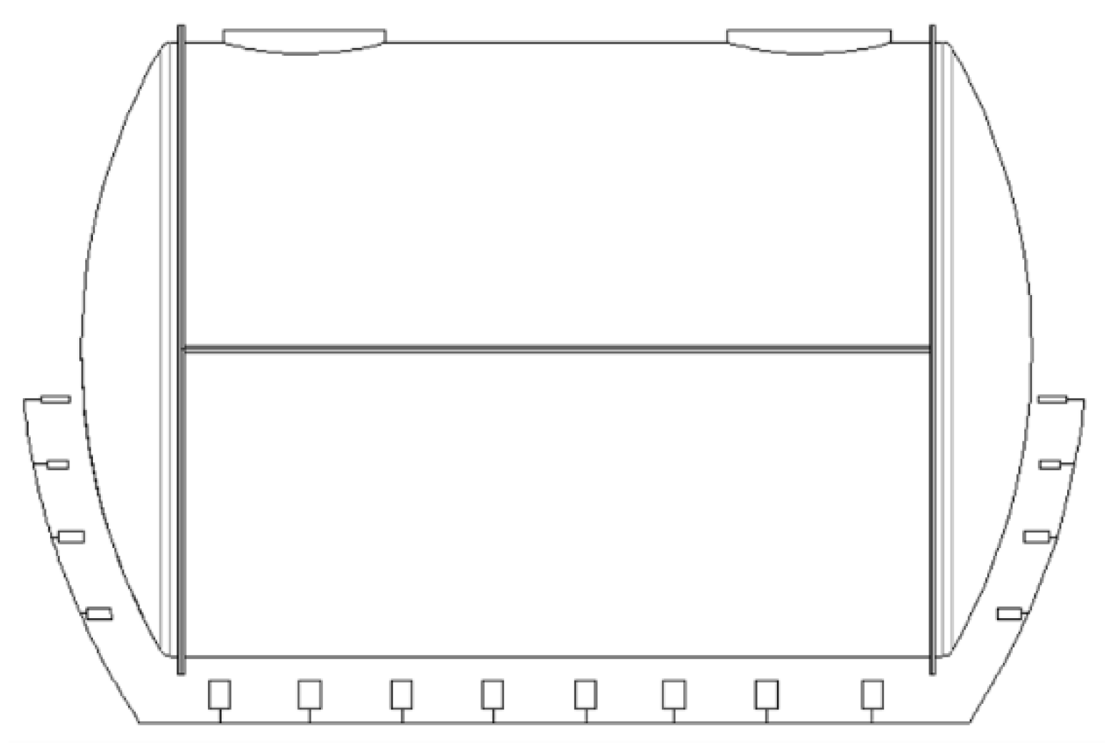
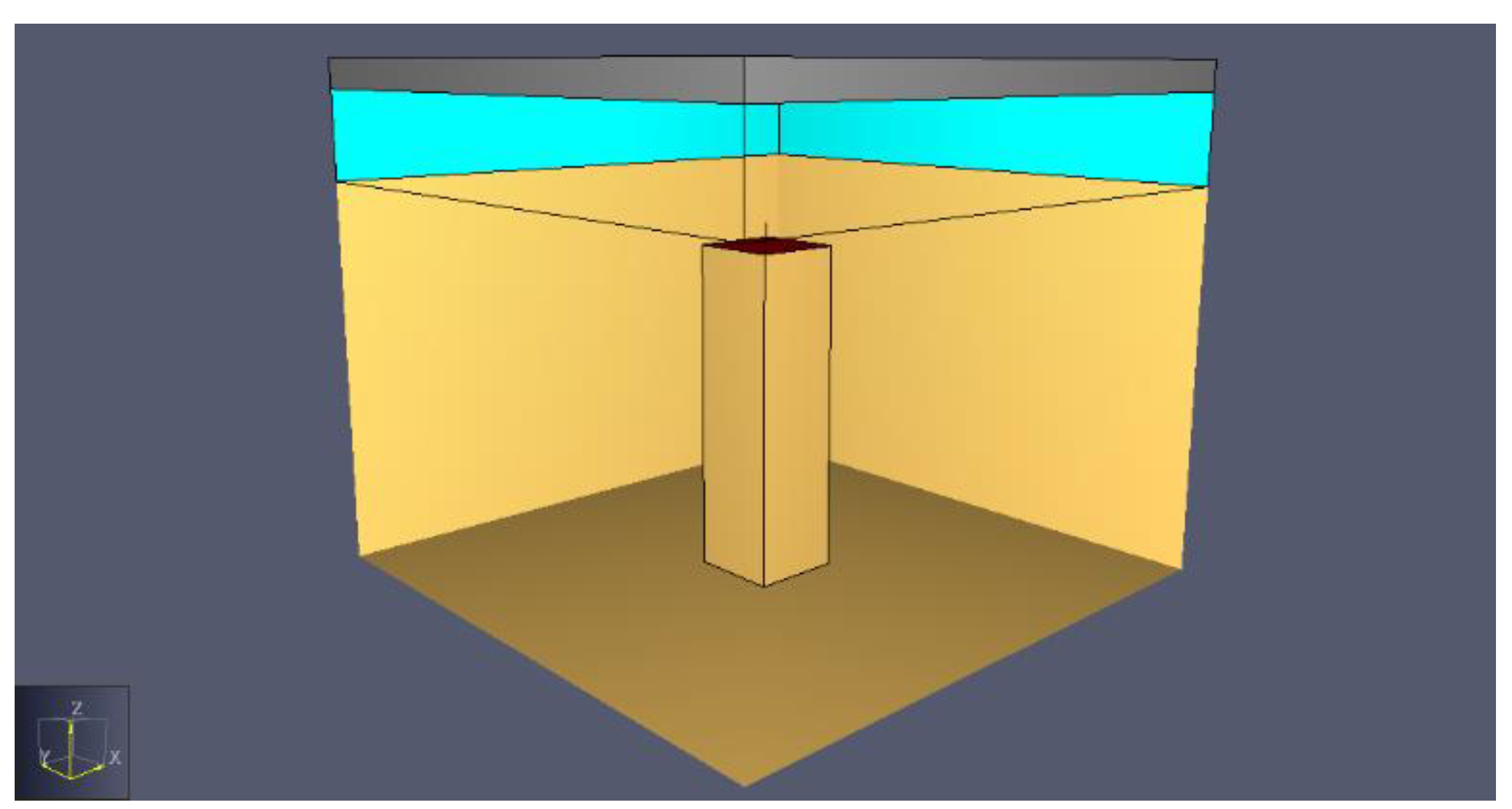
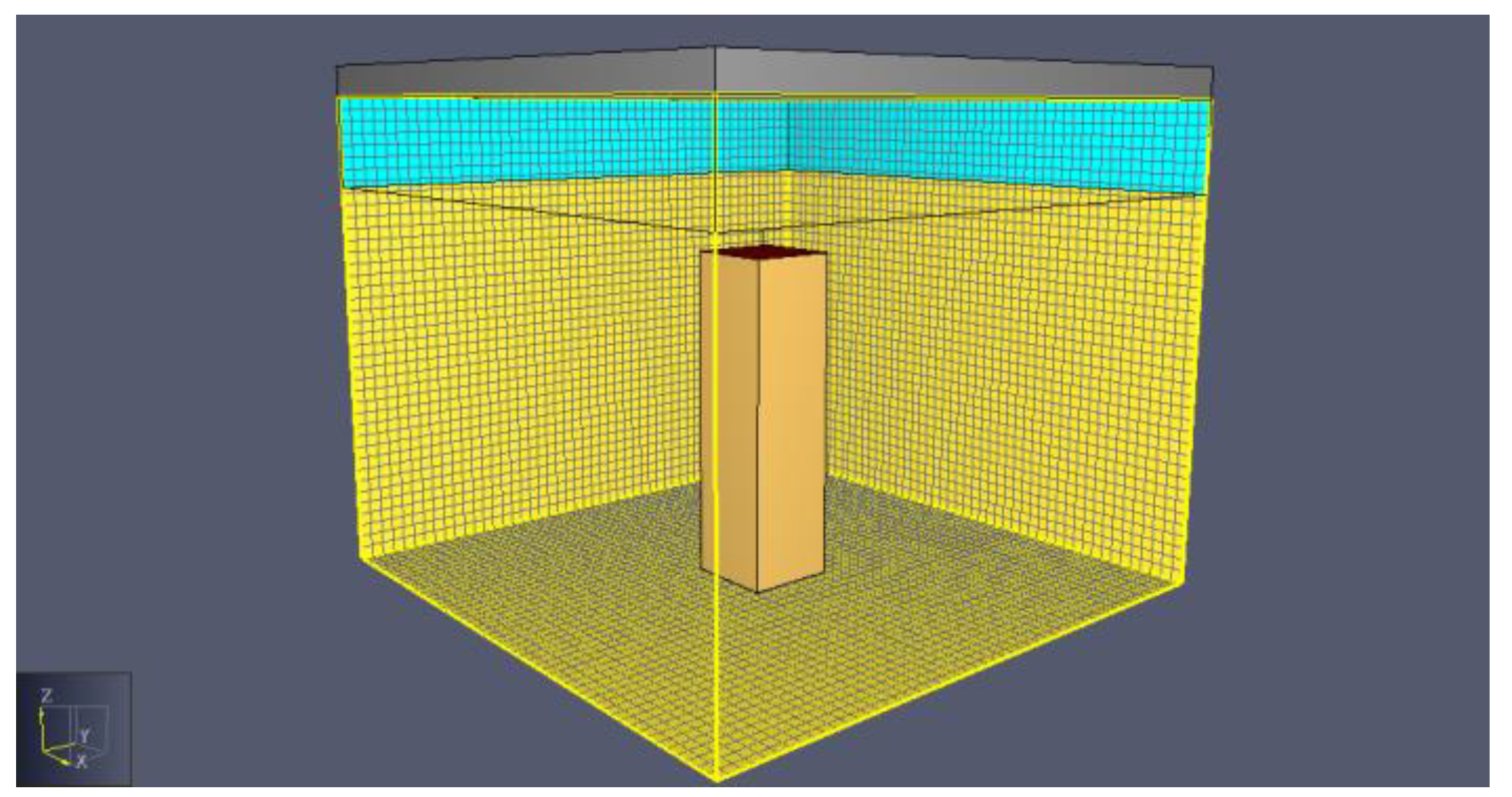
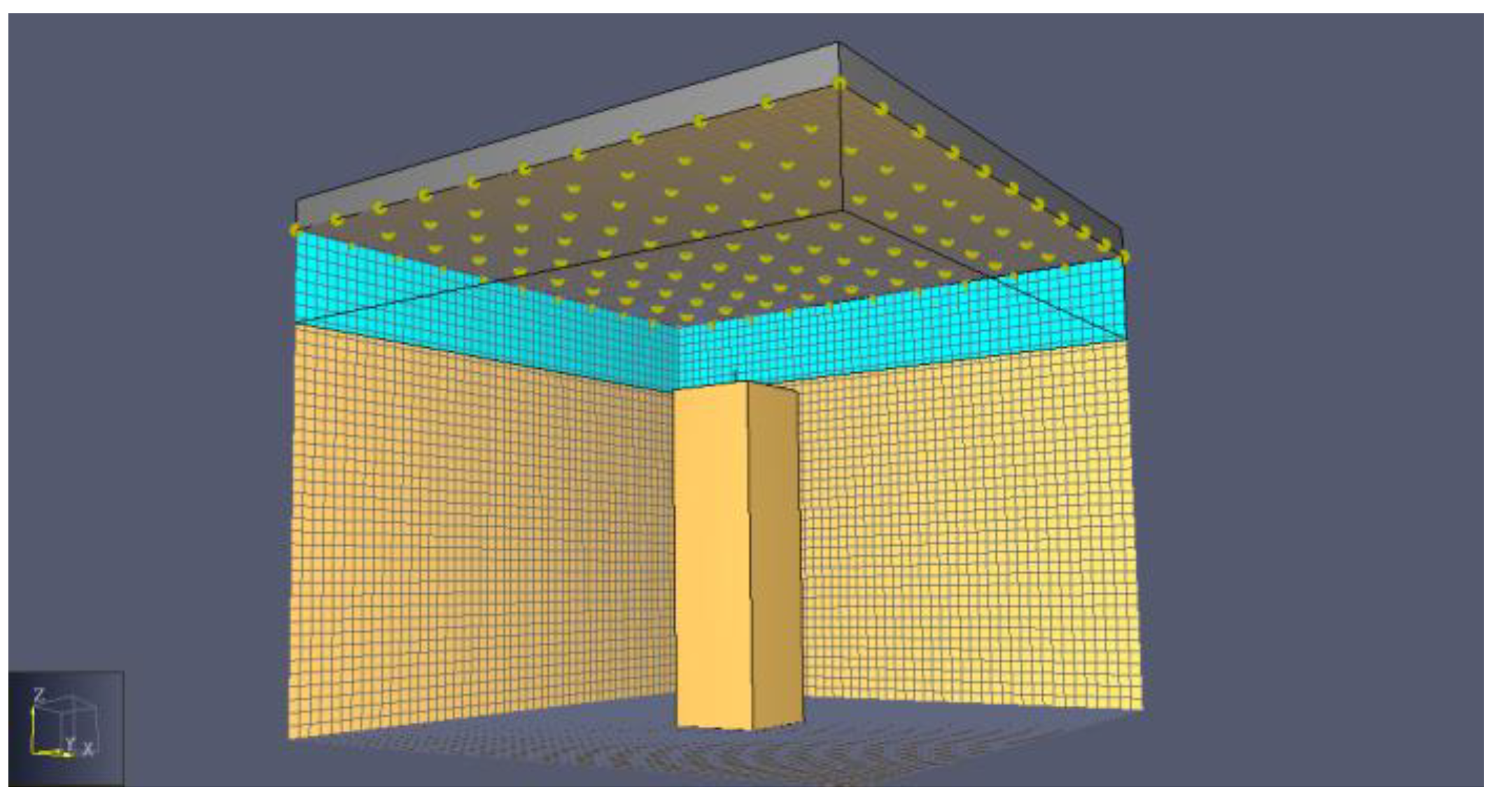
2.1.1. Model Construction and Meshing

According to the principle of mold design and the actual working conditions, the diameter of the 10 m³ rotomolding mold is 2.2 m and the length is 2.7 m. The two ends of the tank are curved structures, and the heating guns are evenly distributed on both sides and below the rotomolding mold, as shown in Figure 1.

FDS software is used to establish the heating model of the heating gun, and only the rectangular structure of the module can be established in the FDS, so the rectangular module substitution method is used for the round heating gun, and the round heating gun is approximated as a square model under the condition of ensuring the same combustion area. The model is shown in Figure 2.

This simulation adopts multigrid division, and according to the principle of grid division of FDS software, the simulation space size is set to 0.2 m × 0.2 m × 0.16 m. For the overall space, a grid size of 4 mm in length, width, and height is selected. The total number of cells is 100,000 after partitioning is completed. After several simulation tests, the grid size meets the simulation requirements. The heating gun heating model is established at the center of the overall space, and the mold model is established at the top of the space. According to the above grid division principles, grid division is carried out, and the grid is divided as shown in Figure 3.

2.1.2. Fuel and Fire Source Setting

(1).

Thermophysical Properties of Natural Gas

Natural gas is a gaseous mixture of various hydrocarbon and nonhydrocarbon substances, of which methane accounts for more than 85%, and is widely used in the rotomolding industry because it is safe, green, and economical. However, different oxygen concentrations and the ratio of hydrocarbons and nonhydrocarbons have a large effect on the thermophysical properties of natural gas during combustion. In this paper, the parameters of the thermophysical properties of natural gas were determined as follows, considering the local hydrocarbon content of natural gas and the oxygen concentration of air: The mass heat of combustion was 13,100 J/g, and the inner and outer flame temperatures were 800 °C and 1000 °C, respectively.

(2).

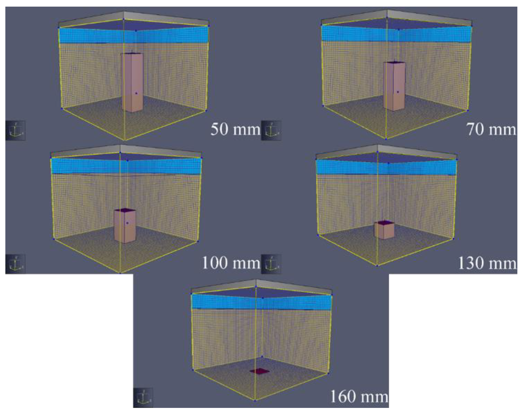
Heating Gun Position Simulation

Taking the 30 mm heating gun as an example, the heating gun was modeled at distances of 50 mm, 70 mm, 100 mm, 130 mm, and 160 mm from the mold, and the distribution of each position is shown in Figure 4.

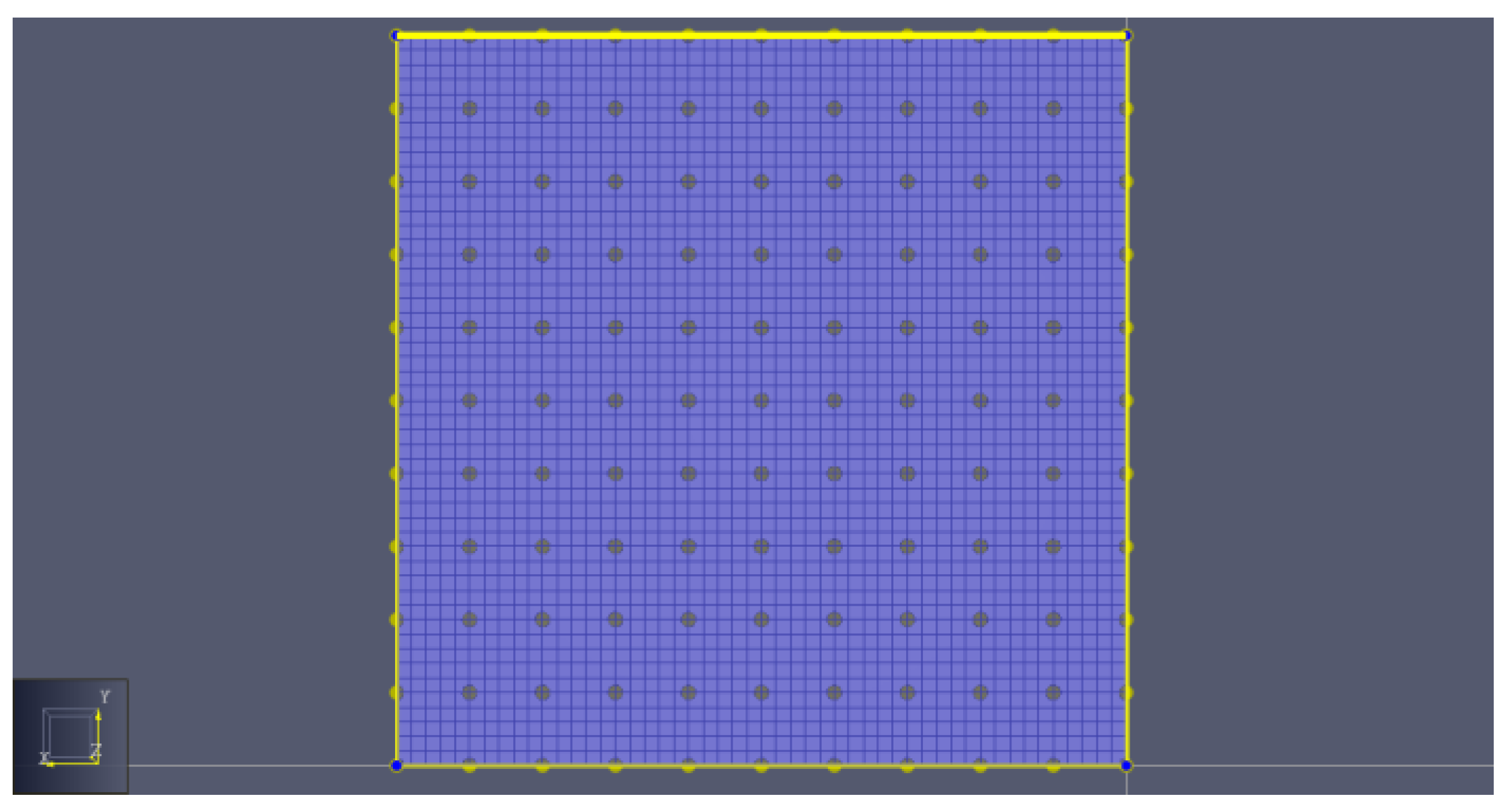
2.1.3. Temperature Detector Settings

The purpose of this section is to study the temperature distribution on the outer surface of the mold after the mold is heated by a heating gun during the rotational molding process. To obtain accurate simulation results, a temperature probe is set on the lower surface of the mold. The arrangement of the temperature detectors is shown in Figure 5. Eleven rows of probes are set on the lower surface of the mold, with each row spaced at 0.02 m; each row contains 11 probes from left to right, with each probe spaced at 0.02 m. In this simulation, a total of 121 temperature sensors were arranged.

2.2. FDS Simulates the Heating Process of Heating Gun

According to the model established in Section 2.1.1, as the simulation space only retains a certain air exchange function around the top and natural gas is a highly combustible substance, when the burner starts to burn, the temperature of the outer surface of the mold will rise rapidly and stabilize. Combined with the structural parameters of the model and the distribution of temperature sensors, the simulation time is set to 50 s, and FDS software is run to simulate.

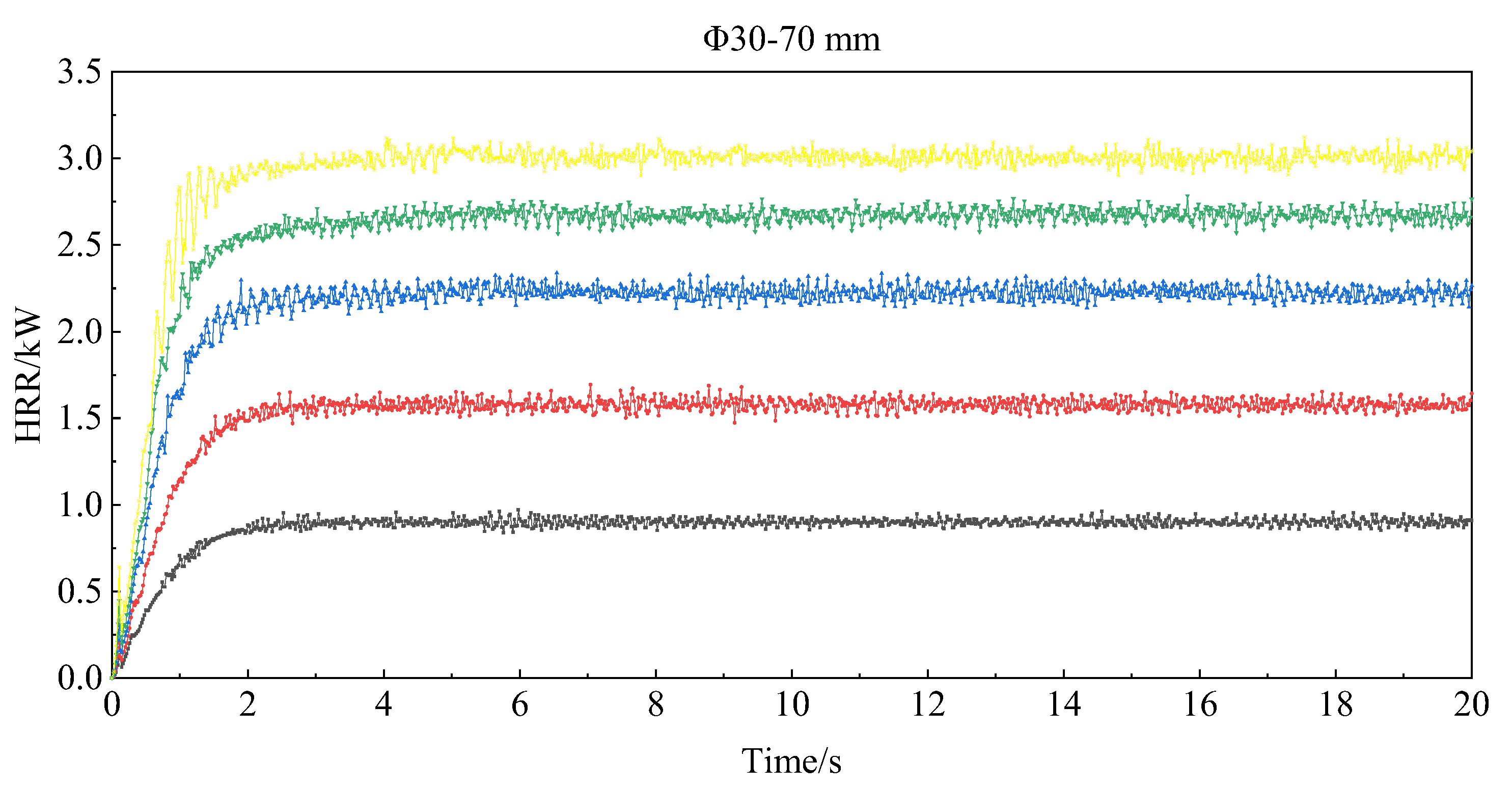
2.2.1. Heat Release Rate

The HRR (heat release rate) is an important indicator to evaluate how fast or slow heat is released during the combustion of materials [12]. The larger the value of the HRR is, the more energy is released during the combustion of the material per unit of time, and the more severe the thermal impact is on nearby objects or media. The HRR–time curves for each diameter heating gun heating phase are shown in Figure 6.

As seen in Figure 6, the HRR curves stabilized after 4 s for all diameter heating guns. Although the heat release rate value exhibits certain fluctuations, always around a certain value change, combustion tends to stabilize. The steady-state heat release rate values for the Φ30 mm, Φ40 mm, Φ50 mm, Φ60 mm, and Φ70 mm heat guns were 0.9 kW, 1.6 kW, 2.2 kW, 2.7 kW, and 3.0 kW, respectively.

2.2.2. Temperature Distribution on the Outer Surface of the Mold

The heating gun and the mold are symmetrical structures, and the distribution of the temperature detector on the lower surface of the mold is shown in Figure 7.

Collating the results of the temperature probe detection showed that the mold surface temperature leveled off after 15 s. The temperature probe value at 20 s was taken to draw a temperature heatmap to analyze the temperature distribution on the lower surface of the mold. By analyzing and filtering the heatmap for each distance of each diameter, the heatmaps for each distance of 30 mm–, 50 mm–, and 70 mm–diameter heating guns were selected, as shown in Figure 8.

(1) During the simulated heating process of the 30 mm heating gun, the heat-affected area gradually decreased with increasing distance from the mold, and the central temperature increased with it. Combining the influence area and the central temperature, a 100 mm distance was selected as the optimal heating distance for the 30 mm heating gun.

(2) During the simulated heating process of the 50 mm heating gun, the heat-affected area did not change substantially with the distance, the central temperature continuously increased with the distance, the edge temperature continuously increased with the distance, and the overall temperature gradient was smoother with the distance. The 130 mm distance was selected as the best heating distance for the 50 mm heating gun, according to the central temperature and overall temperature characteristics.

(3) During the simulated heating process of the 70 mm heating gun, the heat-affected area expanded with increasing distance, the central temperature increased with increasing distance, and the overall temperature gradient was smoother with increasing distance. Combining the heat-affected area, central temperature, and temperature gradient, a 130 mm distance was selected as the best heating distance for the 70 mm heating gun.

3. Thermal Response of Heat-Affected Mold

3.1. Mathematical Model

3.1.1. Thermal Conductivity Equation

(1) Heat conduction follows Fourier’s law [13,14], as shown in Equation (1).

$$Q=-A\lambda \frac{dT}{dn}$$

(1)

where Q is the heat flow rate, W; A is the thermal conductivity area, m²; λ is the thermal conductivity of the material, W/(m·°C); and dT/dn is the temperature gradient, °C/m.

(2) Convective heat transfer follows Newton’s law of cooling, as shown in Equation (2).

$$Q=Ah\left(t-t_f\right)$$

(2)

where h is the convective heat transfer coefficient, W(m²·°C), and t and t_f are the solid surface temperature and fluid temperature, °C, respectively.

(3) Radiant heat transfer obeys the Stefan–Boltzmann law, as shown in Equation (3).

$$Q={\epsilon }_1{A}_1\sigma F_{12}\left(T_1^4-T_2^4\right)$$

(3)

where ε₁ is the object thermal radiation emissivity; A₁ is the area of radiation surface 1, m²; σ is the Stefan–Boltzmann constant; F₁₂ is the shape coefficient from radiation surface 1 to radiation surface 2; T₁ is the absolute temperature of radiation surface 1, K; and T₂ is the absolute temperature of radiation surface 2, K.

3.1.2. Initial and Boundary Conditions

(1) Initial condition: T = T0; T0 is the ambient temperature.

(2) Boundary conditions: In the heating process, the mold-heating surface (outer surface) exhibits convection heat transfer and radiation heat transfer. Therefore, according to Equations (1)–(3) in Section 2.1.1, considering convection heat transfer and radiation heat transfer together, the boundary condition can be expressed as Equation (4).

$$-\lambda \frac{dT}{dn}=h\left(t-t_f\right)+\epsilon \sigma \left[{\left(t+273\right)}^4-{\left(t_f+273\right)}^4\right]$$

(4)

where ε is the integrated radiation coefficient and σ is the Stefan-Boltzmann constant, taken as 5.67 × 10⁻⁸ W/(m²·K⁴).

3.2. ANSYS Model of Heat-Affected Mold

In this section, the ANSYS Workbench platform is used to construct a 3D simulation model of the heat-affected mold to simulate the thermal response of the mold in the heat-affected zone after heat exposure.

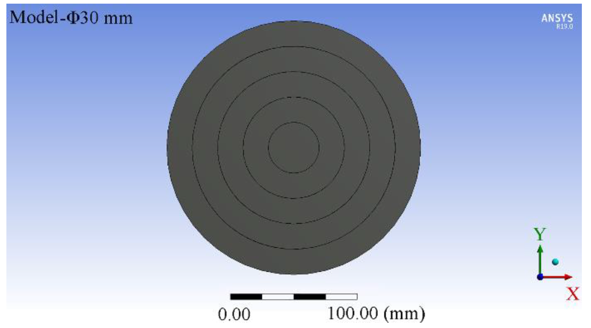
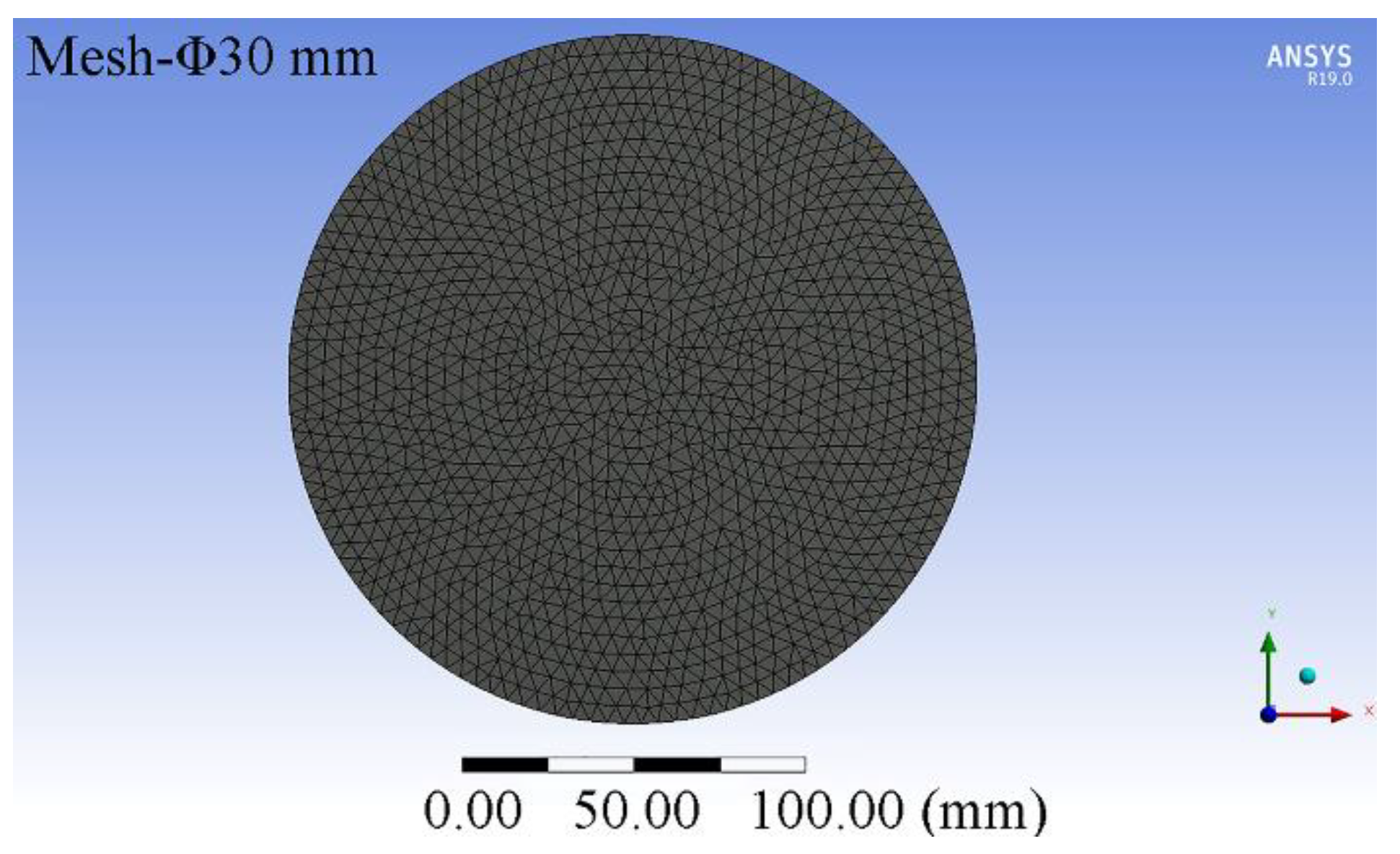
3.2.1. Model Construction and Meshing

The heat-affected mold diameter is D₁ = 0.2 m and the thickness is δ₁ = 10 mm; the material is domestic steel Q235A. The completed ANSYS model is shown in Figure 9. Referring to the relevant literature [15], the physical parameters of the mold materials were determined by combining environmental factors and actual working conditions, and the mold structure and materials are shown in

Table 1. Structure, material, and dimensions of the rotational molding model.

Mold	Material	Diameter/m	Thickness/mm	Density /(Kg·m−3)	Thermal Conductivity /(W·m−1·K−1)	Specific Heat Capacity /(J·Kg−1·°C−1)
Heat-affected mold	Q235A	0.2	10	7850	52.34	434

.

Taking the 30 mm heating gun as an example, in this simulation, the tetrahedral meshing method was chosen for each model as a whole, and the mesh size was divided by a 5 mm mesh through multiple simulations. The mold after the mesh division was completed as shown in Figure 10. As shown in Figure 10, after the model meshing was completed, the total number of nodes was 41,131, and the total number of cells was 24,075.

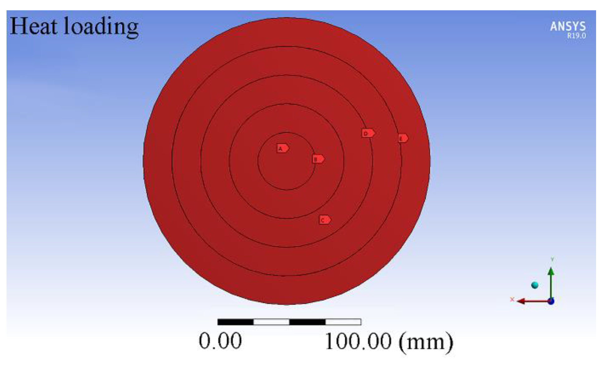
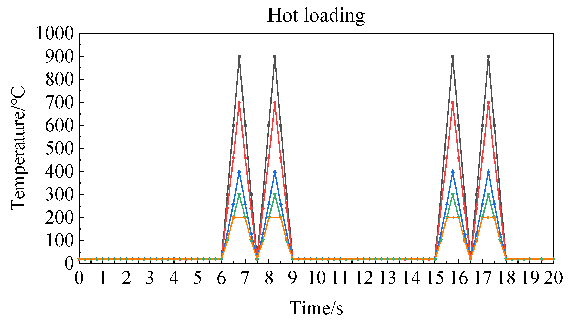
3.2.2. Heating Gun Heating Settings

Since the mold rotates with the spindle and oscillates up and down during the rotational molding process, the heat on the mold surface is a time-varying process, so the transient thermal analysis module is used in this paper [16]. In the simulation, the rotomolding mold was subjected to thermal radiation from the heating gun, and the temperature field distribution on the outer surface of the mold, obtained by solving with the FDS software, was applied to the corresponding ANSYS model locations according to the corresponding zone divisions.

Taking the 30 mm heating gun as an example, according to the optimal heating distance obtained in Section 2.2.2 corresponding to the temperature field situation, different temperatures were loaded onto rings or circles of different diameters, and the heat-affected mold was thermally loaded, as shown in Figure 11.

3.3. Heat-Affected Mold Thermal Response Temperature Field Distribution

The transient thermal module in ANSYS Workbench was used to simulate the distribution of the heating gun end surfaces and the temperature distribution on the inner surface of the model during the heating phase of the heat-affected mold [17].

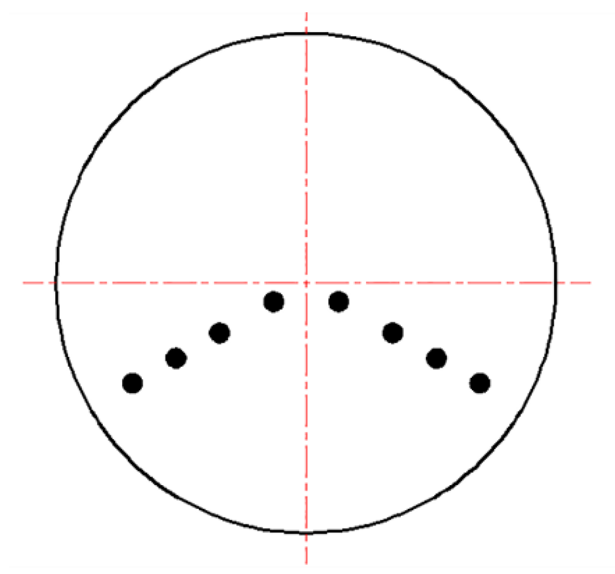
3.3.1. End-Face Distribution of the Heating Gun

In this simulation, the heating guns were chosen to be evenly distributed in two columns on the outer surface of the end-face mold, and the two columns of heating guns were arranged at 120°, as shown in Figure 12.

Since the rotomolding mold rotates with the spindle, the heating curve of the heating gun varies with the end-face diameter. The 30 mm heating gun at 0.15 m from the center of the end face was taken as an example, and the heating curve is shown in Figure 13.

3.3.2. Heat-Affected Mold Temperature Field Distribution

By simulating the heating of 30 mm, 50 mm, and 70 mm heating guns at different diameters on the end face, the position of the 30 mm–70 mm heating guns on the end-face mold was determined. After several simulations, it was determined that the temperature field on the inner surface of the heat-affected mold tended to stabilize in two cycles, so the simulation time was set to three cycles: 27 s. After the setup was completed, the simulation was completed, and the temperature field of the inner surface of the mold was analyzed and filtered by taking 18 s (the second cycle of the heating cycle) for each diameter of the end face, and we obtained 30 mm–0.1 m (30 mm heating gun is 0.1 m from the center of the end face), 30 mm–0.15 m, 50 mm–0.4 m, 50 mm–0.6 m, 70 mm–0.6 m, and 70 mm–0.8 m, as shown in Figure 14.

The figure shows that with the continuation of the heating process, heat accumulates in the mold and affects its inner wall, showing an obvious temperature gradient and the highest temperature in the center.

(1) The inner wall of the 30 mm–0.1 m mold showed six obvious temperature gradients, with a maximum temperature of 335 °C at the center and a minimum temperature of 121 °C at the edges. The inner wall of the 30 mm–0.15 m mold showed five obvious temperature gradients, with a maximum temperature of 239 °C at the center and a minimum temperature of 91 °C at the edges.

(2) The inner wall of the 50 mm–0.4 m mold showed four obvious temperature gradients, with a maximum temperature of 271 °C at the center and a minimum temperature of 123 °C at the edges. The inner wall of the 50 mm–0.6 m mold showed four obvious temperature gradients, with a maximum temperature of 188 °C at the center and a minimum temperature of 103 °C at the edges.

(3) The inner wall of the 70 mm–0.6 m mold showed four obvious temperature gradients, with a maximum temperature of 204 °C at the center and a minimum temperature of 107 °C at the edges. The inner wall of the 70 mm–0.8 m mold showed three obvious temperature gradients, with a maximum temperature of 174 °C at the center and a minimum temperature of 115 °C at the edges.

The linear low-density polyethylene (LLDPE) melting point was 110 °C~125 °C, the heating oxidation temperature was 300 °C, and the best molding temperature was 270 °C [18]. Combining (1)–(3) shows that 30 mm–0.15 m, 50 mm–0.4 m, 70 mm–0.6 m, and 70 mm–0.8 m meet the LLDPE molding conditions.

4. ANSYS Model of the End-Face Mold

4.1. ANSYS Model of the End-Face Mold

In this section, the ANSYS Workbench platform is used to construct a 3D simulation model of the end-face mold to simulate the thermal response of the mold end face after heat exposure [19].

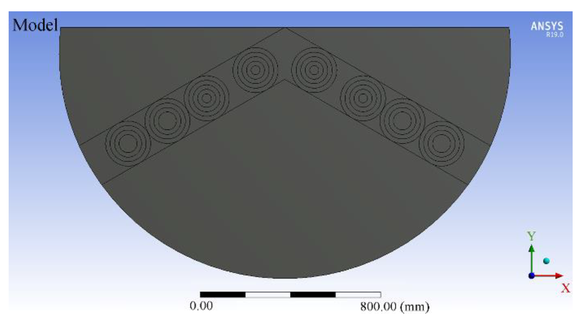
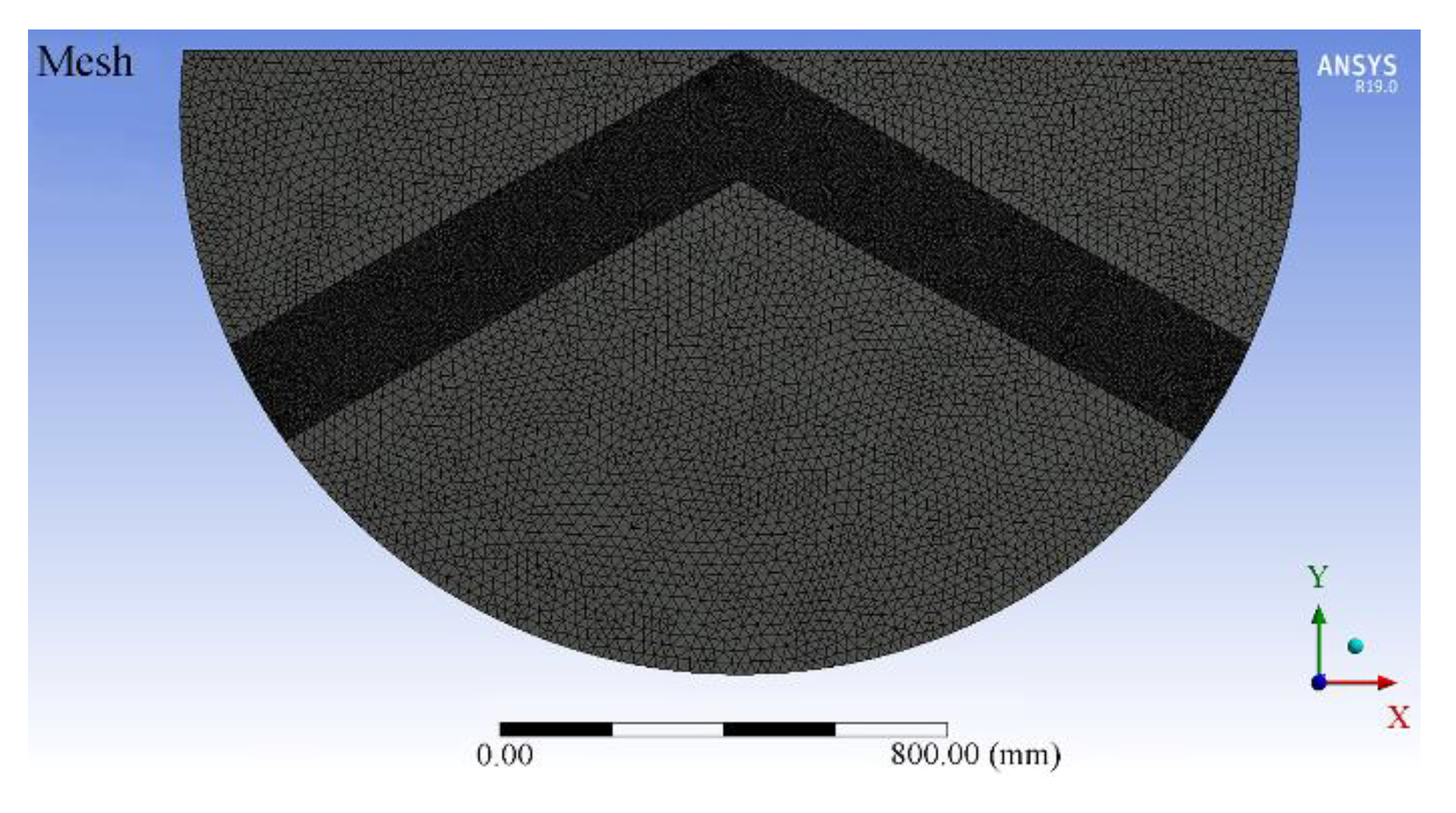
4.1.1. Model Construction and Meshing

The diameter of the heat-affected mold of the heating gun is D₁ = 0.2 m, the thickness is δ₁ = 10 mm, the diameter of the end-face die is D₂ = 2.0 m, and the thickness is δ₂ = 10 mm; the material is domestic steel Q235A. The completed ANSYS model after construction is shown in Figure 15. Referring to the relevant literature [15], the physical parameters of the mold material were determined by combining environmental factors and actual working conditions, and the mold structure and its physical parameters are shown in

Table 2. Structure, material, and dimensions of the rotational molding model.

Mold	Material	Diameter/m	Thickness/mm	Density /(Kg·m−3)	Thermal Conductivity /(W·m−1·K−1)	Specific Heat Capacity /(J·Kg−1·°C−1)
Heat-affected mold	Q235A	0.2	10	7850	52.34	434
End-face mold	Q235A	2	10	7850	52.34	434

.

As shown in Figure 13, 30 mm–0.15 m, 50 mm–0.4 m, 70 mm–0.6 m, and 70 mm–0.8 m heat-affected molds fit inside the end-face molds.

In this simulation, the tetrahedral meshing method was chosen for the model as a whole, and the cell mesh size was set to 20 mm for the whole area of the end-face mold. For the heat-affected mold, the cell mesh size of the selected area was set to 5 mm. After the model meshing was completed, as shown in Figure 16, the total number of nodes was 560,721, and the total number of cells was 327,093.

4.1.2. End-Face Mold Heating Setting

According to Section 3.3.2, 30 mm–0.15 m, 50 mm–0.4 m, 70 mm–0.6 m, and 70 mm–0.8 m heat-affected die heat loading cases were obtained and different temperatures were loaded onto different diameter rings or circles. The end-face die heat loading cases are shown in Figure 17.

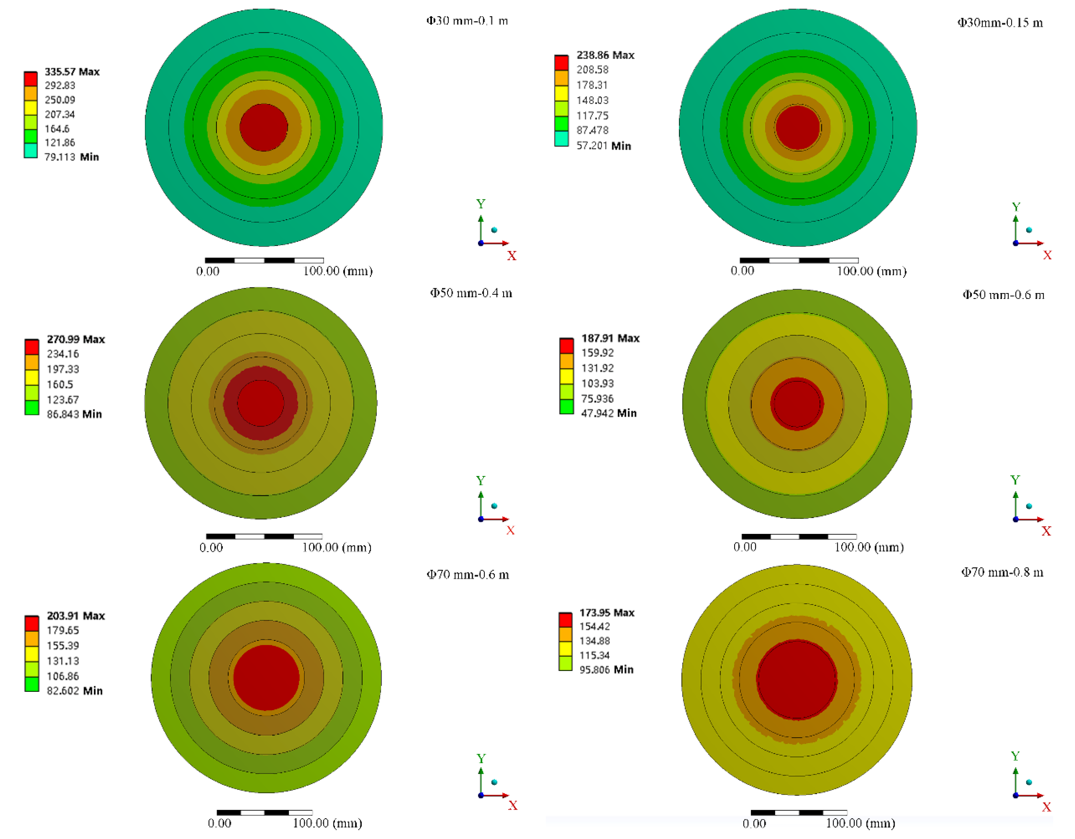
4.1.3. Temperature Field Distribution of the Thermal Response of the End-Face Mold

Using the transient thermal module in ANSYS Workbench, the temperature distribution on the inner surface of the model during the heating phase of the end-face mold was simulated.

Through the heating simulation of the end-face mold as a whole, the thermal influence model was determined in the thermal influence range of the overall end-face mold, and the layout of the heating gun end face is optimized. After several simulations, it was determined that the temperature of the inner wall of the end-face mold tended to stabilize in two cycles, so the simulation time was set to three cycles: 27 s. After completing the setup, simulations were conducted to analyze and filter the internal surface temperature field data at each time point, and Figure 18 shows the temperature field of the internal surface of the end-face mold at 9.5 s and the local enlargement.

Figure 19 shows that the temperature of the inner surface of the end-face mold was substantially higher in the heat-affected mold area, showing a V-shaped temperature band and a clear temperature gradient. Among them, the maximum temperature of 271 °C was at the center of the inner surface of the 50 mm–0.4 m mold, and the minimum temperature of 68 °C was at the edge of the inner surface of the 30 mm–0.15 m mold. However, an obvious heating blind zone was found between the 30 mm–0.15 m mold and the 50 mm–0.4 m mold, and the heat-affected mold distribution did not meet the LLDPE molding conditions.

(1)

The 30 mm–0.15 m model heat-affected area size: Φ120 mm (linear low-density polyethylene (LLDPE) melting point of 110 °C~125 °C [20,21]).

(2)

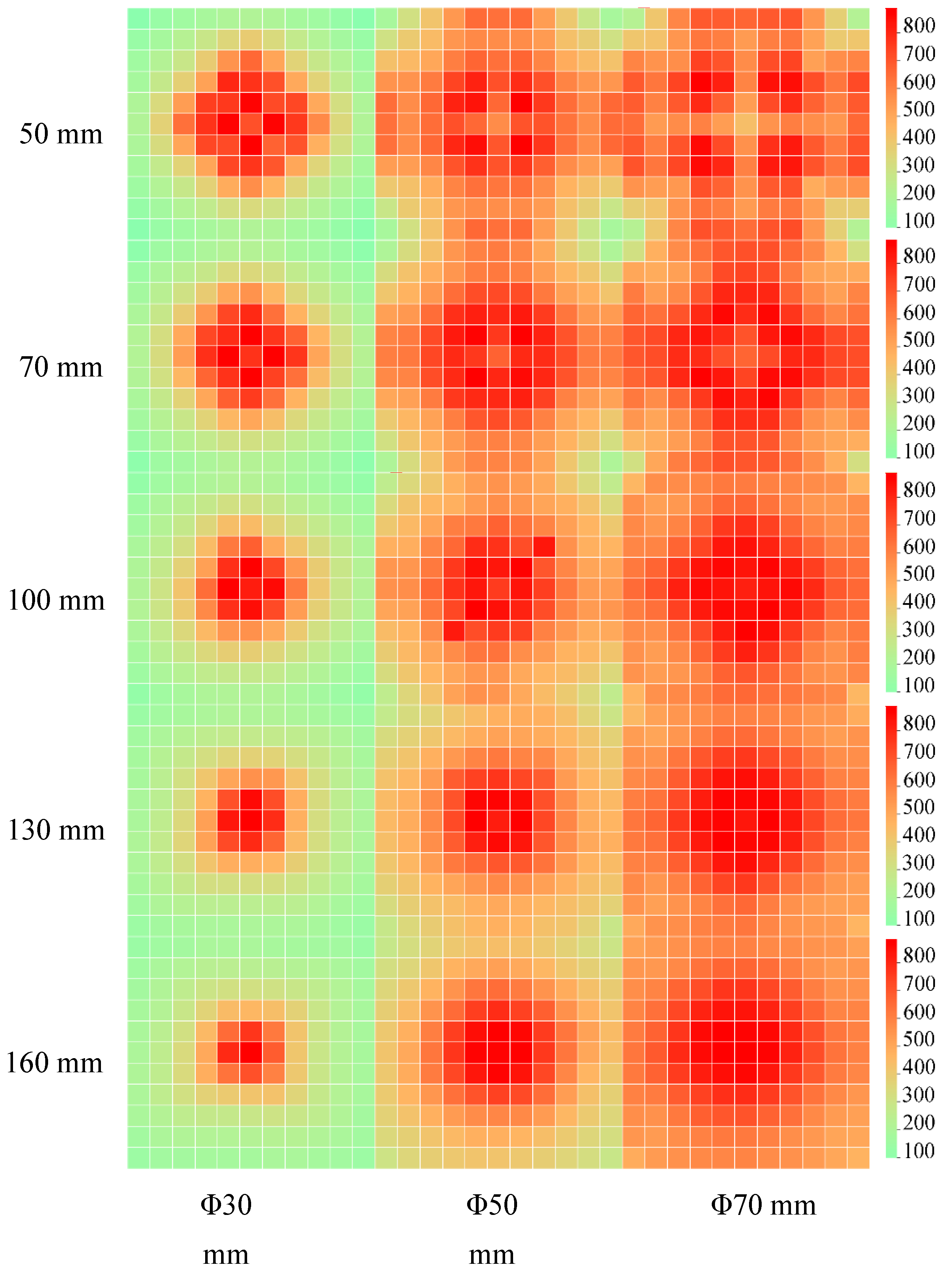
The 50 mm–0.4 m model heat-affected area size: Φ200 mm.

(3)

The size of the heat-affected area for 70 mm–0.6 m and 70 mm–0.8 m molds was Φ200 mm.

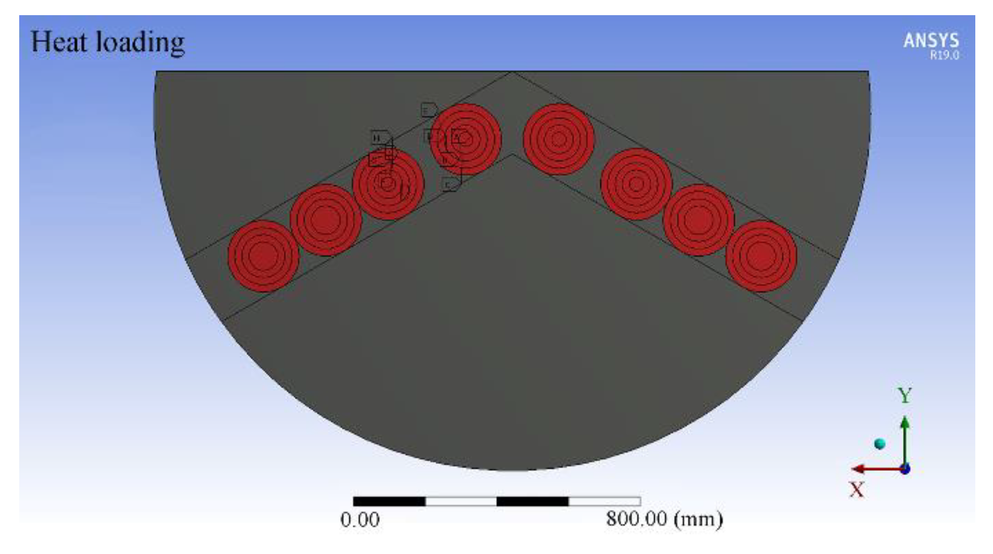
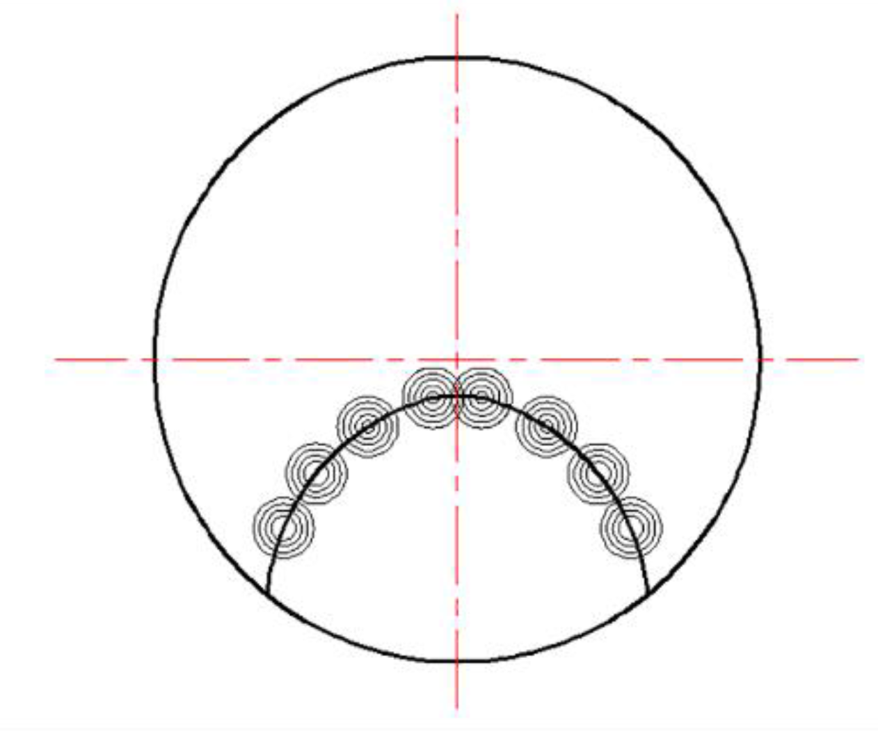
4.2. End-Face Distribution of the Heating Gun

To obtain a better distribution of end heating guns, combining the size of the heat-affected area of the heat-affected mold obtained in the previous section and the actual distribution of rotomolding heating guns [22,23], the distribution of heating guns was set as shown in Figure 19.

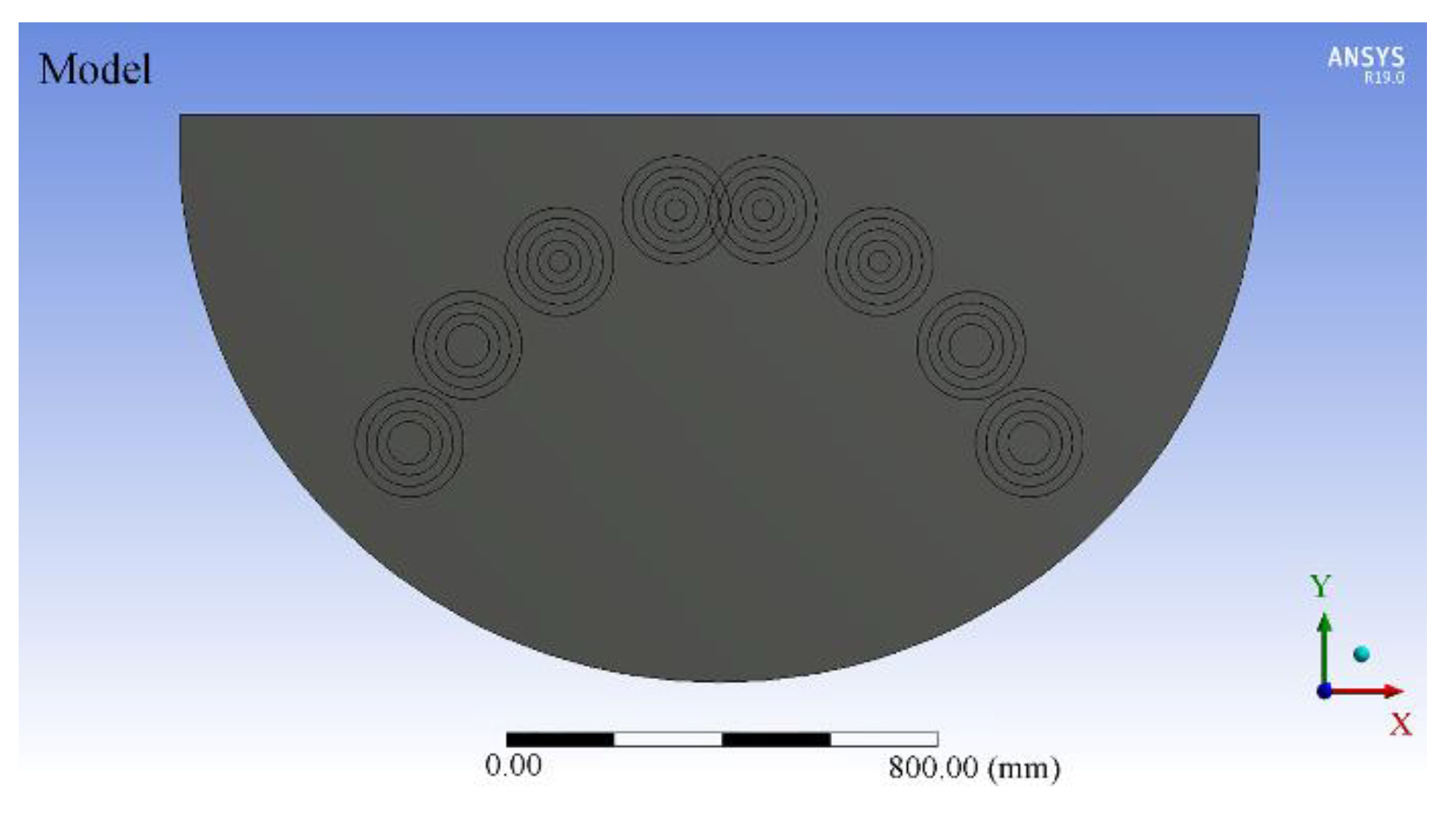
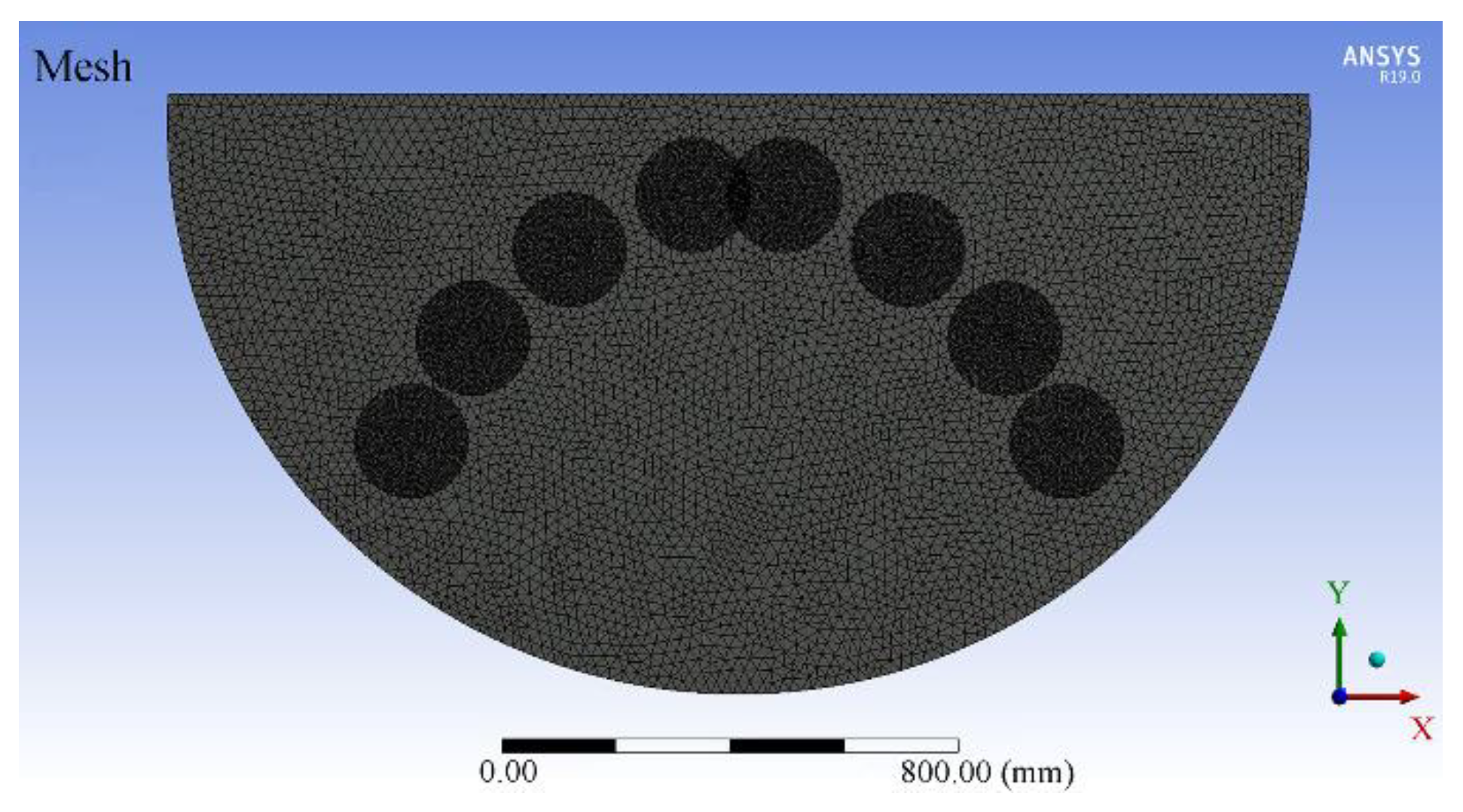
4.2.1. Model Construction and Meshing

The ANSYS heating simulation model is established in Figure 19, and the completed ANSYS model after construction is shown in Figure 20. The diameter of the end die is D₂ = 2.0 m and the thickness is δ₂ = 10 mm; the material is domestic steel Q235A. The 30 mm, 50 mm, and 70 mm heat-affected molds were installed on the end-face molds sequentially according to the distribution of the heating gun end faces in Figure 19. The mold structure and its physical parameters for the end-face mold and heat-affected mold are consistent with Table 2.

As shown in Figure 21, 30 mm–0.15 m, 50 mm–0.4 m, 70 mm–0.6 m, and 70 mm–0.8 m heat-affected dies are assembled inside the end-face mold.

In this simulation, the tetrahedral meshing method was chosen for the model as a whole, and the cell mesh size was set to 20 mm for the whole area of the end-face mold. For the heat-affected mold, the cell mesh size of the selected area was set to 5 mm. After the model meshing was completed, as shown in Figure 21, the total number of nodes was 375,261, and the total number of cells was 215,720.

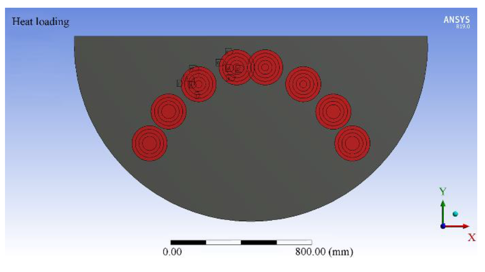
4.2.2. End-Face Mold Heating Setting

In a similar manner to Section 3.2.1, the thermal loading was conducted as follows: The end-face dies were thermally loaded at different temperatures onto rings or circles of different diameters according to the 30 mm–0.15 m, 50 mm–0.4 m, 70 mm–0.6 m, and 70 mm–0.8 m thermally affected die thermal loading cases obtained in Section 3.3.2, as shown in Figure 22.

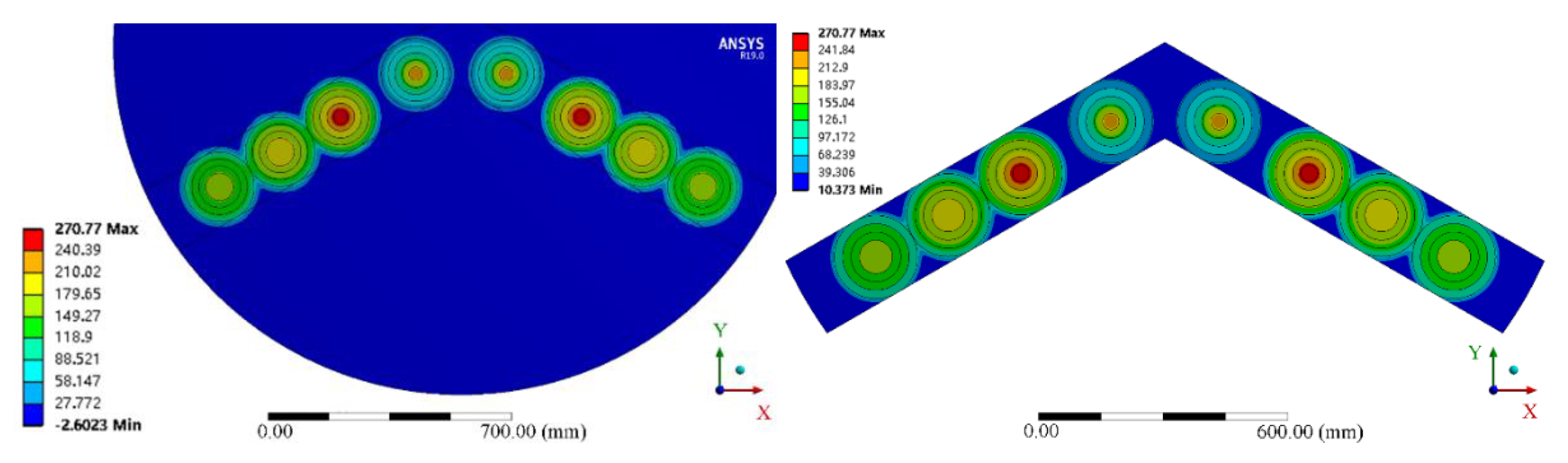
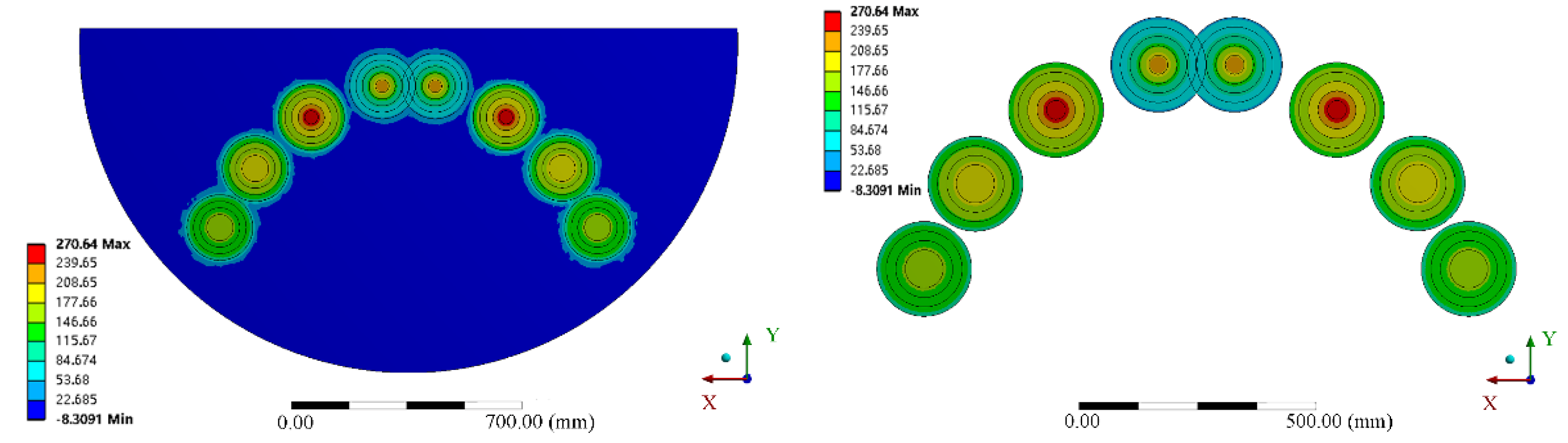
4.2.3. Temperature Field Distribution of the Thermal Response of the End-Face Mold

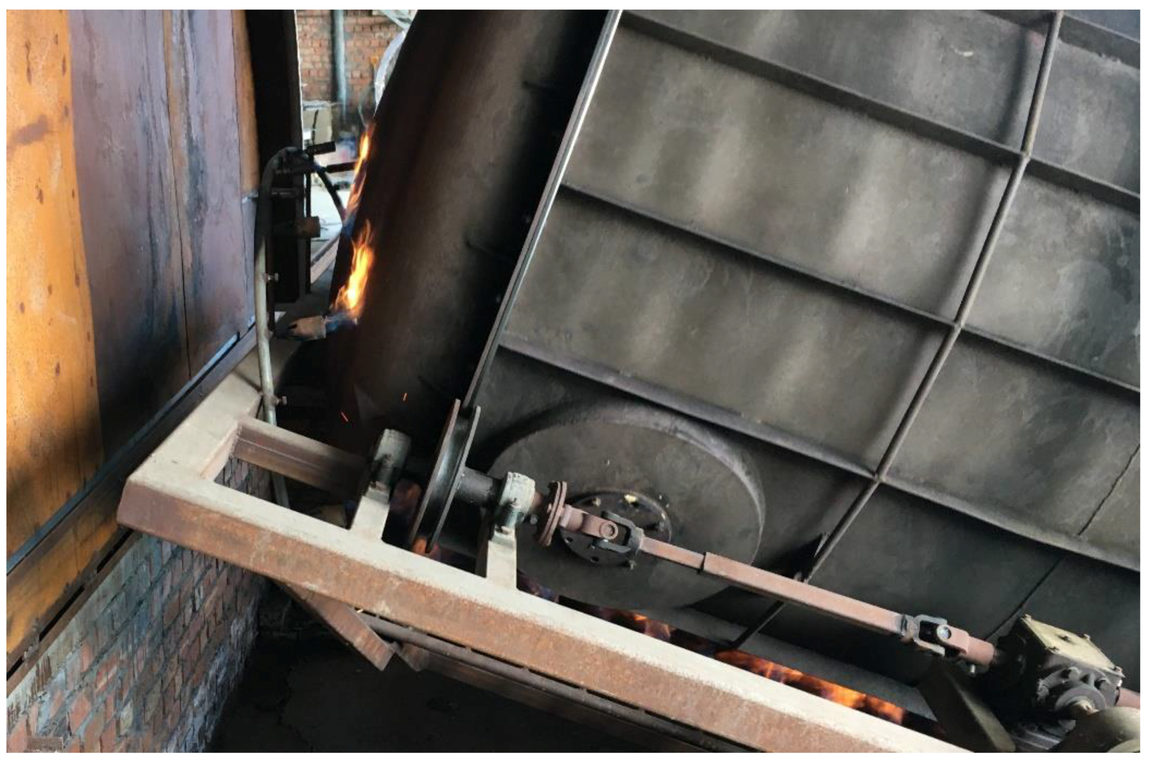
An overall heating simulation of the optimized end-face mold was performed to determine the reasonableness of the optimized heat-affected model end-face layout and to obtain the heating gun end-face distribution. After several simulations, it was determined that the temperature field of the inner surface of the end-face mold tended to stabilize in two cycles, so the simulation time was set to three cycles: 27 s. After completing the setup, the simulation was carried out, and by screening and analyzing the surface temperature at each time, the temperature field and local enlargement of the inner surface of the end-face mold at 9.5 s were taken, as shown in Figure 23.

As seen from Figure 23, the temperature of the inner surface of the end-face mold was substantially higher in the heat-affected mold area, showing a semiarc-shaped temperature band that would affect the temperature of the entire inner surface of the end-face mold with the rotation of the end-face mold. The temperature zone had a maximum temperature of 270 °C in the center area of the inner surface of 50 mm–0.4 m mold and a minimum temperature of 115 °C at the edge of the inner surface of 30 mm–0.15 m mold; the temperature range of the inner surface of 70 mm–0.6 m and 70 mm–0.8 m mold was 146 °C~208 °C.

In summary, the optimized semiarc distribution can effectively meet the LLDPE processing and molding conditions, and in the actual production and processing process, the semiarc distribution is more conducive to the arrangement of the gas transmission pipeline.

5. Experiments

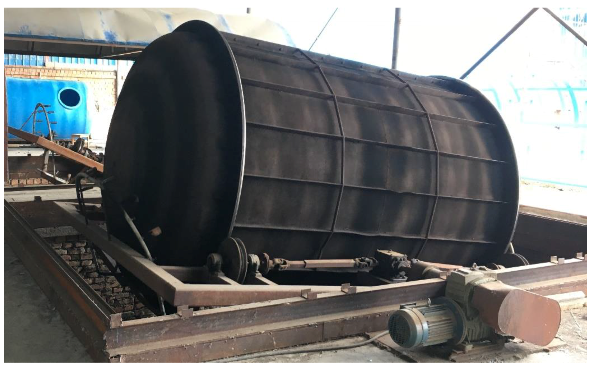
5.1. Experimental Design

The experiments were carried out in the factory of Shihezi Boli Mechatronics Technology Co, Shihezi City, China. The rotomolding device was constructed with reference to the dimensions of the simulation model, and its structure is shown in Figure 24.

The experiments were conducted on the sidewall of a rotomolding mold. The experimental platform consisted of a 10 m³ rotomolding mold, a heating gun set, and a mold support and transmission device. During the experiment, the rotomolding mold was not installed with the right-side end mold, and four infrared temperature sensors were arranged at the original right end surface of Φ0.3 m, Φ0.8 m, Φ1.2 m, and Φ1.6 m to collect the temperature changes of the inner surface of the left end mold.

The heating gun group was located in the mold support and transmission device, the heating gun was installed according to the layout of the simulation-optimized end-face heating gun distribution, and the heating gun end-face layout and heating situation are shown in Figure 25.

The heating gun set was ignited, the heating of the heating gun in the chamber was observed, and the temperature data of each diameter infrared temperature measurement sensor were recorded. The experiment was repeated three times independently, with each heating time lasting 1 min and each cooling time lasting 5 min. The two adjacent experiments were separated by 10 min to allow the mold to cool to ambient temperature, and then the next experiment was conducted after cooling.

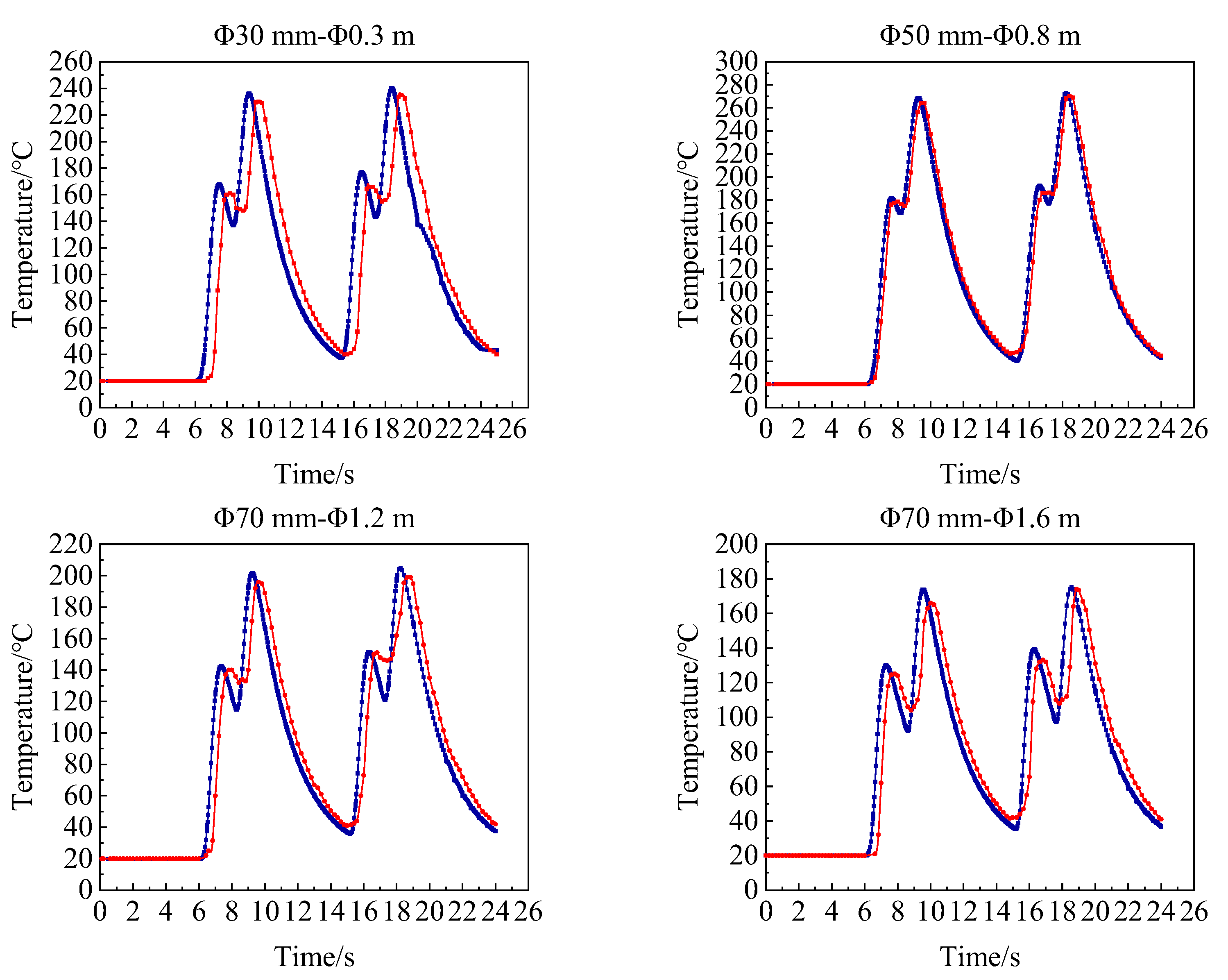
5.2. Experimental Results and Analysis

Four infrared temperature sensors were arranged at Φ0.3 m, Φ0.8 m, Φ1.2 m, and Φ1.6 m on the original right end face with a sampling frequency of 0.2 s/time. The time of igniting the heating gun was recorded as 0 s, and the sampling duration was selected as 27 s with reference to the simulation data.

The experiments were repeated three times independently, the experimental data were averaged and compared with the simulated theoretical values, and the theoretical and experimental temperature variation curves were plotted, as shown in Figure 26. During the data collection process, the rotomolded mold was only open on the right end, resulting in the internal temperature of the mold being higher than the ambient temperature, which had some influence on the collected data. Figure 26 shows that the overall deviation between the theoretical data and the actual collected data was less than 5%.

From the figure, the following observations can be made.

• The experimental data had a certain time delay compared to the theoretical data, with delays of 0.6 s for 30 mm–Φ0.3 m, 0.2 s for 50 mm–Φ0.8 m and 70 mm–Φ1.2 m, and 0.4 s for 70 mm–Φ1.6 m.
• The experimental data had higher peak temperatures and more drastic temperature changes than the theoretical data. In the first wave peak and first trough position (8–10 s), the experimental data curve changed more gently. Higher experimental data were obtained at the second trough and fourth trough positions compared to the theoretical data.
• The comparison and analysis of the data show that the theoretical heat-affected areas of 30 mm–Φ0.3 m and 70 mm–Φ1.6 m were consistent with the actual heat-affected area, and the actual thermal impact areas of 50 mm–Φ0.8 m and 70 mm–Φ1.2 m were larger than the theoretical thermal impact area.

6. Conclusions

This article researched the temperature response of the end-face mold under a heating gun heating condition, proposed the FDS + ANSYS analysis method, and obtained an accurate and effective FDS + ANSYS simulation model. FDS software was used to simulate the heating process of the heating gun, and the thermal diagram of the temperature field of the outer surface of the mold at each distance from the mold for each diameter of the heating gun during the heating process was drawn. the temperature distribution of the heat map was analyzed and the optimal heating distances of the heating gun at Φ30 mm, Φ50 mm, and Φ70 mm were determined to be 100 mm, 130 mm, and 130 mm, respectively. ANSYS Workbench was used to establish the thermal response model of the end-face mold, obtain the temperature field distribution on the inner surface of the end-face mold, and determine the optimal distribution of heating guns at Φ0.30 m, Φ0.80 m, Φ1.20 m, and Φ1.60 m locations on the outer surface of the end-face mold as Φ30 mm, Φ50 mm, Φ70 mm, and Φ70 mm, respectively. Through simulation and experimental verification, the reasonableness of the heating gun end distribution was determined, and the best heating gun end distribution method was obtained.

References

1. Crawford, R.J. Rotational Molding of Plastics, 2nd ed.; Research Studies Press: Taunton, UK, 1996. [Google Scholar]
2. Wen, Y.; Zheng, Y.; Shi, C. Research on the Status quo of Rotomoulding Industry Standards. China Stand. 2018, 7, 125–130. [Google Scholar]
3. Fernandes, C.; Pontes, A.J.; Viana, J.C.; Nóbrega, J.M.; Gaspar-Cunha, A. Modeling of Plasticating Injection Molding–Experimental Assessment. Int. Polym. Processing 2014, 29, 558–569. [Google Scholar] [CrossRef]
4. Habla, F.; Fernandes, C.; Maier, M.; Densky, L.; Ferrás, L.L.; Rajkumar, A.; Carneiro, O.S.; Hinrichsen, O.; Nóbrega, J.M. Development and validation of a model for the temperature distribution in the extrusion calibration stage. Appl. Therm. Eng. 2016, 100, 538–552. [Google Scholar] [CrossRef]
5. Greco, A.; Maffezzoli, A.; Vlachopoulos, J. Simulation of Heat Transfer During Rotational Molding. Adv. Polym. Technol. 2003, 22, 271–279. [Google Scholar] [CrossRef]
6. Sarrabi, S.; Colin, X.; Tcharkhtchi, A. Kinetic Modeling of Polypropylene Thermal Oxidation During Its Processing by Rotational Molding. J. Appl. Polym. Sci. 2010, 118, 980–996. [Google Scholar] [CrossRef] [Green Version]
7. Liu, X. Numerical Study on Heating Phase of Rotational Molding Process. China Plast. 2012, 26, 88–92. [Google Scholar]
8. Wen, Y.; Mao, X.; Wang, Y. Influence of Heating Time on Properties of Rotational Molding Product. Plast. Sci. Technol. 2017, 45, 55–58. [Google Scholar]
9. Liu, X. Analytical Solution of Heat Transfer Model for Heating Phase in Rotational Molding Process. China Plast. 2020, 34, 76–82. [Google Scholar]
10. FDS Networks Group Ltd. Annual Report–December 31, 2008; Reportal: Hong Kong, China, 2009. [Google Scholar]
11. McGrattan, K.B.; Baum, H.R.; Rehm, R.G.; Hamins, A.; Forney, G.P.; Floyd, J.E.; Hostikka, S.; Prasad, K. Fire Dynamic Simulator Technical Reference Guide; National Institute of Standards and Technology Special Publication: Gaithersburg, MD, USA, 2013; pp. 1–3.
12. Zhao, J.; Huang, H.; Qu, K.; Su, B. Research on thermal radiation response of large crude oil tank based on numerical simulation method. J. Cent. South Univ. (Sci. Technol.) 2017, 48, 1651–1658. [Google Scholar]
13. Zhang, L.; Xie, P.; Ding, Y.; Jiao, Z.; Qin, L.; Yang, W.; College of Mechanical and Electronic Engineering, Beijing University of Chemical Technology. Research and Application of Wireless Temperature Measurement Equipment for Rotational Molding Machine. Eng. Plast. Appl. 2013, 41, 70–72. [Google Scholar]
14. Shao, S.; Qi, S.; An, Q. Thermal Conductivity of PE-LLD/CF Composite. China Plast. 2009, 23, 46–49. [Google Scholar]
15. Zhou, Y.X.; Lu, Z.L.; Zhang, M.; Zhao, X.C.; Fan, Z. Study on the tribological behavior of Monel alloy. Ordnance Mater. Sci. Eng. 2004, 5. [Google Scholar] [CrossRef]
16. Zhang, G.; Hu, R.; Chen, J. ANSYS 10.0 Thermal Finite Element Analysis Guide Window Stutorial; China Machine Press: Beijing, China, 2007; pp. 2–3. (In Chinese) [Google Scholar]
17. Wu, G.X.; Ma, Q.W.; Taylor, R.E. Numerical simulation of sloshing waves in a 3D tank based on a finite element method. Appl. Ocean. Res. 1998, 20, 337–355. [Google Scholar] [CrossRef]
18. Yang, Y. Simulation and Optimization of Gas Phase Polymerization Process for LLDPE. Chem. Enterp. Manag. 2020, 1, 175–177. [Google Scholar]
19. Yang, Y.F.; Zheng, J.; Jia, C.Z.; Liu, C.C. Analysis on Gun Barrel Heat Conduction Finite Element Simulation. J. Gun Launch Control 2011, 1, 45–48. [Google Scholar]
20. Zhang, L. Studies of Equipment and Processes of Large Plastics Rotational Molding; Beijing University of Chemical Technology: Beijing, China, 2014. [Google Scholar]
21. Hejna, A.; Barczewski, M.; Andrzejewski, J.; Kosmela, P.; Piasecki, A.; Szostak, M.; Kuang, T. Rotational Molding of Linear Low-Density Polyethylene Composites Filled with Wheat Bran. Polymers 2020, 12, 1004. [Google Scholar] [CrossRef] [PubMed]
22. Lucas, A.; Danlos, A.; Shirinbayan, M.; Motaharinejad, V.; Paridaens, R.; Benfriha, K.; Bakir, F.; Tcharkhtchi, A. Conventional rotational molding process and aerodynamic characteristics of an axial-flow hollow blades rotor. Int. J. Adv. Manuf. Technol. 2019, 104, 1183–1194. [Google Scholar] [CrossRef]
23. Jiang, X.; Lin, Y.; Huang, S. Rotational Moulding Process and Die Deign of Fuel Tanks. Plastics 2017, 46, 49–51. [Google Scholar]
Figure 1. Rotational molding model.
Processes 10 00097 g001
Figure 2. FDS model.
Processes 10 00097 g002
Figure 3. Mesh division.
Processes 10 00097 g003
Figure 4. FDS model for each distance.
Processes 10 00097 g004
Figure 5. Spatial layout of the temperature detector.
Processes 10 00097 g005
Figure 6. HRR-time curve of the heating stage of each diameter heating gun. Yellow—Φ70 mm, green—Φ60 mm, blue—Φ50 mm, red—Φ40 mm, brown—Φ30 mm.
Processes 10 00097 g006
Figure 7. 2D distribution of temperature detectors.
Processes 10 00097 g007
Figure 8. Heatmap.
Processes 10 00097 g008
Figure 9. ANSYS heat-affected mold.
Processes 10 00097 g009
Figure 10. Meshed 3D model in ANSYS.
Processes 10 00097 g010
Figure 11. Hot loading of mold.
Processes 10 00097 g011
Figure 12. Distribution of the end surfaces of the heating gun.
Processes 10 00097 g012
Figure 13. Temperature–time curve of hot loading. Orange: Φ160 mm–Φ200 mm, green: Φ120 mm–Φ160 mm, blue: Φ80 mm–Φ120 mm, red: Φ40 mm–Φ80 mm, black: Φ40 mm.
Processes 10 00097 g013
Figure 14. Distribution of temperature on the inner surface of the model.
Processes 10 00097 g014
Figure 15. ANSYS end-face mold.
Processes 10 00097 g015
Figure 16. Meshing of the model.
Processes 10 00097 g016
Figure 17. Hot loading of the mold.
Processes 10 00097 g017
Figure 18. Distribution of temperature on the inner surface of the model.
Processes 10 00097 g018
Figure 19. Distribution of the end surfaces of the heating gun.
Processes 10 00097 g019
Figure 20. ANSYS end-face mold.
Processes 10 00097 g020
Figure 21. Meshing of the mold.
Processes 10 00097 g021
Figure 22. Hot loading of the mold.
Processes 10 00097 g022
Figure 23. Temperature field distribution on the inner surface of the mold.
Processes 10 00097 g023
Figure 24. Rotational molding device.
Processes 10 00097 g024
Figure 25. Distribution of the heat gun.
Processes 10 00097 g025
Figure 26. Theoretical and experimental temperature–time curves. Blue: theoretical curves, red: experimental curves.
Processes 10 00097 g026