
Optimal Darwinian Selection of Microorganisms with Internal Storage


1
Inria, INRAE, Université Côte d’Azur, Sophia Antipolis, 06902 Valbonne, France
2
Biocore Team, CNRS, Sorbonne Université, 06230 Villefranche-sur-Mer, France
3
Laboratoire de Mathématiques d’Avignon (EA 2151), Avignon Université, 84018 Avignon, France
4
Laboratoire d’Océanographie de Villefranche (LOV), CNRS, Sorbonne University, IMEV, 06230 Villefranche-sur-Mer, France
*
Author to whom correspondence should be addressed.
Processes 2022, 10(3), 461; https://0-doi-org.brum.beds.ac.uk/10.3390/pr10030461
Submission received: 19 January 2022
/
Revised: 11 February 2022
/
Accepted: 14 February 2022
/
Published: 24 February 2022
(This article belongs to the Special Issue Mathematical Modeling and Control of Bioprocesses)
Abstract
:In this paper, we investigate the problem of species separation in minimal time. Droop model is considered to describe the evolution of two distinct populations of microorganisms that are in competition for the same resource in a photobioreactor. We focus on an optimal control problem (OCP) subject to a five-dimensional controlled system in which the control represents the dilution rate of the chemostat. The objective is to select the desired species in minimal-time and to synthesize an optimal feedback control. This is a very challenging issue, since we are are dealing with a ten-dimensional optimality system. We provide properties of optimal controls allowing the strain of interest to dominate the population. Our analysis is based on the Pontryagin Maximum Principle (PMP), along with a thorough study of singular arcs that is crucial in the synthesis of optimal controls. These theoretical results are also extensively illustrated and validated using a direct method in optimal control (via the Bocop software for numerically solving optimal control problems). The approach is illustrated with numerical examples with microalgae, reflecting the complexity of the optimal control structure and the richness of the dynamical behavior.
1. Introduction
The interaction between species coexisting in an ecosystem is complex and affected by external factors. Depending on their environment, some species will dominate, while others, less adapted, will progressively decline. This Darwinian pressure, when it can be manipulated [1], provides the opportunity of guiding the evolution of species of interest. This concept can be applied to artificial ecosystems to select individuals with a desired trait. Here, we focus on microalgae, unicellular photosynthetic microorganisms with promising potential for industrial applications [2,3]. The great biodiversity of microalgae opens the door for a large range of applications [4]. They are grown for their pigments, antioxidants or essential fatty acids [5], and, over the longer term, their efficient way of producing proteins, bricks for green chemistry, biofuel and CO mitigation [2,6,7]. To date, microalgae do not have the place they deserve in biotechnology (see, e.g., [8,9,10]) and many optimization steps must be carried out to improve the economic and environmental performances of these processes at a large scale [6,11]. Currently, only wild organisms sampled in nature are used on an industrial scale. One of the key challenges is to improve the productivity of these strains.
Species in agriculture have been improved after centuries of selection and hybridization. The objective of this work is to develop an alternative approach adapted to microorganisms to select, on a shorter time scale, more productive microalgae strains, by Darwinian pressure. The idea is based on the competitive exclusion principle in a continuous reactor [12] stating that the species which more efficiently uses the available resources will win the competition. The conditions for a bacterial or microalgal species to win the competition for a limiting substrate have been well established, and the outcome of the competition is known to depend on the minimum requested substrate to support a growth rate equal to the dilution rate [12,13].
Experimental works for maintaining a long-term selection process to favour individuals of interest have already been carried out [14,15]. Since the experiments can last several months or several years, these approaches are costly in time. There is a margin of improvement by applying optimal control theory [16] to enhance the selection process for N strains competing for the same resource (the control parameter being the dilution rate).
One main issue is to decrease the operating time when the species of interest starts to dominate. Several works addressed the question of improving the selection process in minimal time in the case of the chemostat system with Monod’s laws [17,18]. Microalgae are more complicated microorganisms better represented by the Droop model, taking into account the internal accumulation of the limiting nutrient [19,20]. Such a model for two strains in competition leads to a five-dimensional problem. The minimal time selection problem with this model is the main focus of the paper. It has been tackled in [21,22] after a simplification allowing for reducing the model dimension. This necessitated to oversimplify the initial dynamics which can play a role in the minimal time selection.
Optimal control [23] strategies ensuring the domination of the strain of interest are derived using the Pontryagin maximum principle [24]. Since the system is affine w.r.t. the control, we obtain various possible structures for an optimal control, namely, the concatenation of several bang arcs or of a bang arc with a singular arc of first order satisfying Legendre–Clebsch’s condition. The paper is structured as follows: in Section 2, we introduce the model and present the optimal control problem. We also prove the reachability of the target set. In Section 3, we make explicit the necessary conditions provided by the Pontryagin Maximum Principle and we introduce properties of the switching function. A thorough study of singular arcs is provided in Section 4 thanks to geometrical control theory. The paper is concluded with numerical simulations of optimal strategies using a direct method in Section 5.
2. The Optimal Control Problem (OCP)
2.1. Droop Model and Main Assumptions
We consider the Droop model [19]. This emblematic variable yield model represents the growth rate of microorganims which can intracellularly store nutrients. When two strains are in competition, it results in a five-dimensional system. The growth of each strain depends on the intracellular quota-storage (q-variable) of the limiting nutrient (s-variable). More precisely, when two species/strains, of biomass concentrations and are competing for one limiting nutrient s in the bioreactor, the Droop model reads as follows:
where is the quota storage of the i-th species and is the input substrate concentration. The dilution rate is a bounded non-negative control function such that , where is the maximal admissible value of the dilution rate, above the maximum actual growth rates [22] (this will be made more precise in Section 2.3) of the two species as shown in Figure 1. In addition, for , is a non-negative function representing the rate of substrate absorption, i.e., the uptake rate of the free nutrient s, and is also a non-negative function representing the growth rate of the i-th species (see [25]).
Following for instance [25], we suppose that the uptake rates are expressed as,
which corresponds to Michaelis–Menten’s kinetics. Here, the parameters and are positive, . In addition, we assume that, for , there is such that cell division does not occur if . Concerning the Droop model, the kinetics are defined by
In addition, for , let stand for,
and let , be such that , (observe that , are uniquely defined). Thus, one has,
System (1) satisfies the following invariance property.
Proposition 1.
Proof.
First, observe that, for , never vanishes whenever . Now, is clearly invariant by the dynamics of since (resp. ) whenever (resp. ). Similarly, for :
where the last inequality follows from the choice of and the fact that , . This ends the proof. □
The parameter represents the maximum internal storage quota. Since is invariant by (1) (Proposition 1), we notice that stands for the effective maximum internal storage quota for . Thus, in the sequel, we consider without loss of generality that for . In the sequel, we also assume that , fulfill the following hypothesis:
Assumption A1.
The affinity of species 1 for the substrate is higher than the one of species 2, i.e., , or equivalently:
From (2), we deduce that, for ,
It means that species 1 with the lower absorbs nutrients slightly faster.
We are now in a position to formulate the OCP of interest.
2.2. Statement of the Optimal Control Problem (OCP)
In this work, we suppose that the first species (with biomass concentration ) is the one of interest. Our aim is to compute the best feeding strategy, that is, the optimal (dilution rate) control function , such that becomes predominant in the photobioreactor in minimal-time. This can be formulated and quantified in terms of the ratio between the two competing species. Intuitively, we wish to find an adequate control strategy (if possible optimal) for which, at the end of the process, we have .
Firstly, the set of admissible controls is defined as,
where is the space of locally integrable functions on every compact on and is the maximum pump feeding capacity. In practice, is designed above the maximum growth rates of the coexisting species (see Section 2.3).
To handle the selection process between the two species, let us define a subset of as,
We choose the parameter such that in such a way to quantify the contamination rate of the interesting strain . Whenever a trajectory reaches the target set , this means that the biomass of the first species is significantly greater than the other one when reaching the target at the terminal time (if possible).
Objective 1.
The optimal control problem (OCP) can then be stated: determine a dilution-based control strategy in such a way that trajectories of (1) starting from an initial condition within the set reach the target set in minimal-time, i.e.,
where is the unique solution of (1) associated with such that and is the first entry time of into the target set. In the sequel, we will use the simpler notation instead of .
In other words, for every positive initial conditions such that , we are seeking an admissible control strategy , steering the trajectory of the system (1) from to the target set in minimal-time, for a fixed (Figure 1) and a given contamination rate . Note that, if one is able to synthesize such an optimal control for every , then one is able to construct an optimal feedback control over as . Such an optimal control problem falls into the class of minimal-time control problems governed by a mono-input affine controlled system, for which the synthesis of an optimal feedback control, thanks to geometric control theory, is a crucial (but also delicate) issue. In particular, handling the high dimension of the Droop model in competition and its resulting optimality system is challenging. Note also that the linearity of the problem w.r.t. D (in contrast, for instance, with strictly convex cost functionals) leads to technicalities because singular arcs usually occur in this setting, see Section 4.
2.3. Basic Properties
We now introduce the so-called actual growth rates. These key functions will have an important role in the optimal separation strategy. For that, let us firstly start with the following observations:
- •
- The mapping is one-to-one with ;
- •
- For every , one has and is one-to-one from into ;
- •
- It follows that the composition such thatis well-defined and is also one-to-one;
- •
- Hence, the mapping such thatis well-defined over with values in and is one-to-one.
From these observations, one can immediately check that the mappings , and are increasing.
Indeed, for , one can write with and
which implies that is increasing. The actual growth rate of species i is then defined as the mapping ,
The resulting generic functions are illustrated in Figure 1: Let us now define,
Throughout the paper, we suppose that satisfies the following assumption.
Assumption A2.
There is a unique such that for every and for every . In addition, Δ has a unique maximum .
Taking into account that , the inequalities satisfied by according to Assumption A2 can also be written:
If we assume that s is regulated to using an appropriate control D, we notice that the q-variables are regulated to some unique , for . The unique point , where , plays a crucial role in the optimal control strategy of (OCP) as discussed in Section 5. Finally, (the maximum dilution rate) is assumed to be large enough in order to drive competition between the two species. More precisely, we assume that satisfies the hypothesis:
Assumption A3.
The maximal value of the dilution rate satisfies
These assumptions will ensure reachability (as detailed in the next section) of the target , and establishes a generic framework where both species may win the competition for sufficiently large time (considering for instance various constant control parameters D that favor species 1 or 2). Thus, under these considerations, we ensure the well-posedness of the optimal control problem of interest. In this general framework, the objective is then to determine the optimal D that steers the trajectories in minimal-time to the desired target.
2.4. Reachability of the Target
Our next aim is to show that the target is reachable from every initial condition. First, let us recall that the set
is an invariant and attractive manifold for (1) for a given persistently exciting control (i.e., an admissible control function such that ).
Proposition 2.
For every initial condition , there exists an admissible control and a time such that , where is the unique solution of (1), starting from , associated with .
Proof.
Let and . Without any loss of generality, we may assume that . Indeed, observe that is not a steady-state of whenever over or over . Thus, if we apply (in that case ) or (in that case ), then is reached in a finite horizon. Consider the feedback control function,
in such a way that the unique solution of (1) associated with this control satisfies for every time (Cauchy–Lipschitz’s Theorem). We claim that there exists large enough such that for every time . Indeed, when , taking into account (8), it follows:
Now, when , it is easy to see that converges to , since satisfies the linear ODE ). At steady-state, we thus have
In conclusion, when ,
or, equivalently, using that, at steady state, that is, , we end up with
Thanks to Assumption A3, this last expression is upper bounded by for t large enough, which proves our claim. Finally, posit and observe that
It follows that when , which implies that . This ends the proof. □
2.5. Motivation of Studying the OCP
Thanks to Proposition 2, the target set is reachable from any initial condition, thus the existence of an optimal control of (6) is standard (namely because the dynamics is affine w.r.t. the control): it is an application of the Fillipov Theorem, see, e.g., [26,27,28]. Considering such a control as in the proof of Proposition 2 then indeed allows the system to let the species of interest dominate the reactor, but this process can be long (see, for instance, Example 1). Another possible strategy is to use a constant control D. Following [12], depending on the value of D, species 1 may win the competition, i.e.,
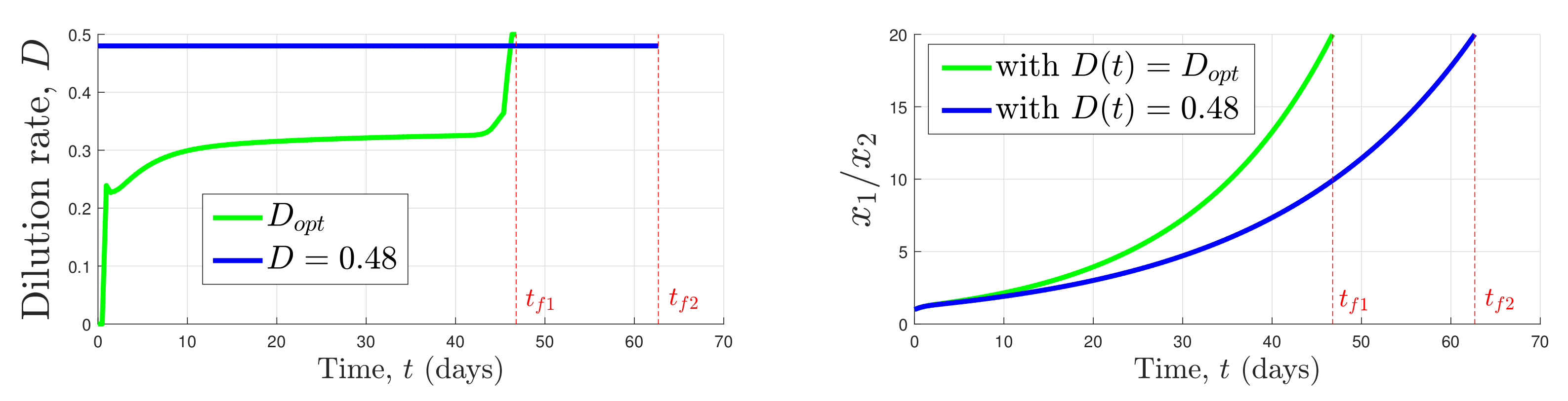
In that case, this (simple) strategy indeed allows for reaching the target. However, this convergence is asymptotic and depends on the value of D as in the competitive exclusion principle. Roughly speaking, if (where and are such that and ), then species 2 wins the competition, whereas, if , species 1 wins the competition. We refer to [12] for more details about the asymptotic behavior of (1) for a constant control D. Thus, the target set may not always be reachable with a constant control D. Our objective in this paper is precisely to propose a methodology to compute a control strategy to reach the target set faster, playing on the control as illustrated in Figure 2.
Example 1.
Let us consider the following parameters: , , , , , , , , . The contamination rate is fixed to . The initial conditions are given by: , and . As illustrated in Figure 2, the target is reached after days using the control , while dominates the culture after days using the constant control . Let us also point out that, using an arbitrary constant control , we are not even sure that wins the competition (trajectories do not reach the target in that case).
3. Necessary Conditions on Optimal Controls
We start this section by generalizing previously obtained results [22,29] characterizing optimal solutions of (6). For that, we apply the PMP which allows for obtaining necessary conditions satisfied by optimal controls of (6). We denote by and , respectively, the state and adjoint variables (also called co-state or covector). The Hamiltonian associated with the optimal control problem
is given by
Let and let be an optimal pair such that reaches the set in a time . Thanks to the PMP, there exist an absolutely-continuous map and such that:
- The pair is non-trivial, i.e., .
- The covector satisfies
- The Hamiltonian maximization condition writes
- At the terminal time, the transversality condition writes:
Here, stands for the normal cone to at some point , see [28]. The adjoint Equation (9) is equivalent to:
We define an extremal as a quadruplet such that is non zero and such that (1) and (9)–(11) is verified. Whenever , we say that the extremal is abnormal; if , then we say that the extremal is normal. Because (6) is autonomous (i.e., the system does not depend explicitly on time), the Hamiltonian computed along an extremal is constant. In addition, since the terminal time is not fixed, we classically obtain, following optimal control theory, that .
The transversality condition is crucial for obtaining properties on optimal controls by reasoning backward in time from the terminal time . We shall next extend earlier results [22] by taking into account explicitly the fact that is a half-space of and exploiting that belongs to the set (the boundary of the target set). Then, condition (11) can be transformed more explicitly as follows. At , the normal cone to writes
Therefore, inclusion (11) is then equivalent to
together with
and the inequalities and . Actually, one has and . Suppose indeed that . Then, (14) would imply , and, since (9) is linear w.r.t. , we would obtain over . Using the constancy of H, we would also obtain contradicting the PMP. We can then conclude that
Throughout the paper, we suppose that only normal extremals occur, i.e., , and, without any loss of generality, we may assume that (up to a renormalization of the necessary conditions that are linear w.r.t. ).
Remark 1.
Abnormal extremals are not generic. They correspond to the optimal path reaching the target set in some particular subset of the target set and are such that (and thus ). From the conservation of H, this implies that in such a way that is not uniquely defined in contrast with the normal case (see below). At such a singular point, the value function (the minimal time as a function of ) is also non-differentiable.
Going back to the normal case, i.e., , the covector at can be completely determined (thanks to the conservation of H) as follows:
Notice that the quantity is non-zero along a normal extremal. As a consequence, the transversality condition (11) coupled with the conservation of H are equivalent to (16). The computation of at is useful to integrate the state adjoint system backward in time from the target set.
We now wish to exploit the Hamiltonian condition (10). It is of particular interest to introduce the switching function, which allows us to determine the optimal control D according to the sign of the switching function. For that, let us denote by the switching function:
associated with the control function .
for a.e. . In the case where , resp. over a time interval , we say that the optimal control u is of bang type (denoted by , resp. ). When the control is non-constant in every neighborhood of a time , we say that is a switching time, and one must have . Next, when the switching function vanishes over a time-interval , we state that a singular arc occurs. In this case, the corresponding trajectory is singular over , and such an arc will be denoted by . Singular arcs are essential to optimize the time to steer an initial condition to the target set. Now, we are ready to state some main features of the switching function , and then investigate properties of the singular paths.
Lemma 1.
- (i)
- The function is continuously differentiable over and, moreover,
- (ii)
- At the terminal time , it holds:
Proof.
By differentiating w.r.t. t, we find that
Remark 2.
Following the formalism of geometric control theory, never involves D explicitly, but D is present in the expression of , , see [27]. If is the first integer for which the control is present in the expression of , we usually say that the singular arc is of order k.
At this step, an optimal control is a concatenation of bang and singular arcs:
with possibly infinitely many crossing times (in particular, if there is a singular arc of order 2 [27]). The occurrence and properties of singular arcs as well as the various (possible) structure for an optimal control of (6) will be precisely the matter of the next section. The goal is to reduce (if possible) the number of possible structures for an optimal control.
4. Singular Arcs and Insights into Optimal Solutions
4.1. Legendre–Clsebsch’s Necessary Condition and Computation of the Singular Control
The analysis of singular arcs requires to compute . Indeed, the Hamiltonian condition does not give any information about an optimal control during a singular phase. Thanks to the next computations, we shall also be able to deduce an expression of the singular control during a singular arc.
Doing so, let us define as
Hereafter, to simplify the layout, we do not write the dependency of , s, , , w.r.t. the time. To shorten the notation, we also do not write explicitly the dependency of certain functions w.r.t. some variables. Using (12)–(18), one can write
Lemma 2.
- (i)
- The derivative of can be expressed as:
- (ii)
- The second derivative of fulfills the equality:
Proof.
By differentiating w.r.t. t, we have
Note that these computations have been verified thanks to a symbolic computation software. The next step is to establish whether Legendre–Clebsch’s condition is verified or not along a singular arc. Recall that this condition is necessary for optimality and that it can be stated as follows (see, e.g., [27,30,31]).
Theorem 1
which is fulfilled over .
(Legendre–Clebsch’s condition [27]). Let be such that the trajectory is singular over . Then, one has:
Using the expression of the derivative given in (22), we provide in the next lemma the expression of the second derivative, .
Lemma 3.
Let be such that the trajectory is singular over . Then, one has:
Proof.
Proposition 3.
over and Legendre–Clebsch’s condition (with a strict inequality) is fulfilled over .
Along a singular arc that occurs over a time interval , it holds that:
Proof.
Because the trajectory is singular over , one has over this interval; thus, satisfies:
It follows that over . In a left neighborhood of , one has from (12) ; thus, since vanishes at , we necessarily have in a left neighborhood of . Because is zero over , we deduce that over (at , vanishes at , as well as ). Over , we note that
hence does not vanish over . Suppose that vanishes over at a time . Then, one must have since over . However, at , the adjoint equation implies that
because , over , , and over . This is a contradiction and thus does not vanish over . Assumption A1 implies that , thus over as desired. We can then conclude that Legendre–Clebsch’s condition (with a strict inequality) is fulfilled over the whole interval . □
A consequence of the previous proposition is that, when a singular arc occurs over some time interval , then it is of order 1. Based on this proposition, we shall only consider singular arcs of first order in the remaining of the paper. If Legendre–Clebsch’s condition holds true, the singular arc is said to be of turnpike type [26]. The expression defining the singular control can then be derived using (22). Next, let be defined by:
We now give an expression of the singular control as a feedback of the state and covector.
Proposition 4.
Proof.
This expression follows from (22) in which is replaced by and (since ). □
Corollary 1.
If the singular arc occurs over some time interval , expression (26) simplifies into
where is given by
and, in this case, simplifies also into because .
Remark 3.
- (i)
- Note that Legendre–Clebsch’s condition (with a strict inequality) is equivalent to (and that this condition is always verified over with close to .
- (ii)
- In view of the general expression giving the singular control, see (26), there is no guarantee a priori that the singular control is always with values in , i.e., that the singular arc is always admissible (even if Legendre–Clebsch’s condition is verified). This can bring additional difficulties; however, we may discard this point by choosing large enough.
- (iii)
- Notice that (27) is at least active at in the case where a singular arc steers the model trajectories towards the target , since the transversality conditions ensure that .
4.2. About the Occurrence of a Terminal Singular Arc at the Terminal Time
The aim of this section is to discuss the possibility of having a singular arc over some time interval (with ) and the structure of optimal controls. Our main questioning is as follows:
Does any optimal trajectory contain a singular arc over some time interval ?
To analyze this point, let us summarize properties of the switching function at (that are consequences of transversality conditions associated with the codimension 1 target):
- The switching function and its derivative vanish at :
- The second derivative of the switching function satisfies:
- In addition, Legendre–Clebsch’s condition (23) is always satisfied along a singular arc defined in a left neighborhood of the terminal time .
The necessary conditions (28) and (29) are a very good indication for the occurrence of a singular arc and are thus strong arguments to answer positively to the above question. Thus, we could now wonder whether or not conditions (28) and (29) are sufficient to ensure the occurrence of a singular arc in some time interval . It appears that this question is complex and falls into the setting of geometric optimal control theory. As far as we know, such conditions are not equivalent to the occurrence of a singular arc over some time interval (this may depend, in particular, on the initial condition). It is, however, worth mentioning that these conditions (in particular (28)) are commonly used numerically to implement a singular arc in shooting methods [32]. In our context of Droop model, it is very interesting to notice that singular arcs are the cornerstone of the optimal control, in particular for a large set of initial conditions that are biologically meaningful (typically for heterogeneous cultures where ). However, the answer to the above question is not always true and depends on the initial condition (as it has been confirmed using direct optimization methods, see Section 5). Indeed, as illustrated in Example 2—Section 5, when the initial conditions are taken very close to the target (, and , the singular arc does not appear or appears marginally at to satisfy the transversality conditions.
Recall that . Hence, the sign of depends on that is computed in the next lemma.
Lemma 4.
At the terminal time, one has
In addition, the second derivative of the switching function exists at and:
Proof.
We can now define the function:
From the previous lemma, we deduce the behavior of an optimal path near the terminal time:
- First, the target set can only be reached at some point such that (30) is fulfilled.
- In addition, if , then, in a left neighborhood of , the optimal control is of bang type and satisfies
- If a singular arc occurs in a left neighborhood of , then one must have , i.e., a singular arc reaches the target in the subset of defined as:
4.3. Toward an Optimal Synthesis Characterizing the Optimal Solutions
Reducing the number of switching times is in general non-tractable for nonlinear optimal control problems governed by a system in dimension greater than three. Nevertheless, thanks to the properties of singular arcs, we obtained previously and of the switching function at , we can expect a limited number of possible structures for an optimal control as we formulate in the next conjecture.
Conjecture 1.
Every initial condition in is steered optimally to the target set via a control D that has a finite number of switching times. In addition, for almost every initial condition, an optimal control presents the following structure:
For a large set of initial conditions in some subset (far from the target), there is a single bang arc and a terminal singular arc, whereas, for some initial conditions close to the target set, no singular arc occurs (i.e., is of zero duration).
This conjecture has been verified numerically for a large number of initial conditions (see Section 5). Our argumentation to confirm this conjecture is as follows.
- From the PMP, we have seen that, for every initial condition in , an optimal control is a concatenation of bang arcs and singular arcs .Moreover, since the switching function satisfies the strong requirements ,(from the transversality conditions) as well as Legendre–Clebsch’s condition, we conjecture that, for almost all initial conditions, an optimal control is singular in a left neighborhood of the terminal time. This implies in particular that the number of switchings is finite since we proved that any terminal singular arc is of first order. In addition, the number of switchings is minimal in general (apart when chattering occurs, see [27], which is not the case here). Thus, an optimal control should be of type with one or two bang arcs before the terminal singular arc.As we have seen, we also must have , which only involves state variables at the terminal time. This surprising condition mixing the first derivative of the basic functions in the Droop model, with the s variable on one side and the variables on the other side, is, however, hard to interpret biologically.
- For some marginal—-but admissible—initial conditions outside of , the structure of an optimal control of (6) may be of bang type for almost all , or , with very small (see, e.g., Example 2 in the next section). This is the case when typically , i.e., the initial condition is very close to the target set , with in addition . Thus, the requirement is easily satisfied. Thus, in this particular situation, it comes as no surprise that the fastest path to reach the target is the one exploiting the fact that (since ) along with , since it maximizes (we recall that ).
It is worth noticing that, when no singular arc occurs, the strategy mainly consists of “pushing” and as quickly as possible towards the target using , when the initial conditions and are very close to . Nevertheless, this strategy may not be the optimal one whenever and are “far” from satisfying . This is typically the case illustrated in Example 3 in the next section.
For an optimal control of type , the occurrence of a singular arc is related to the so-called turnpike phenomenon that we now explain in this framework. For a large subset of initial conditions that are biologically the most relevant, the structure of the optimal control is bang-singular. The singular arc is the control given in (27) that reaches the target . Moreover, this singular phase coincides with optimal trajectories that stay most of the time close to the critical point defined in Section 2.3 (related to the actual growth rates and the function ). Observe, for instance, the trajectories s, and in Figure 3a.We also believe that the concatenation of bang arcs before the major singular phase exclusively aims at moving towards . Then, the singular arc takes over at a switching-time instant and ensures that the associated singular trajectory, denoted , satisfies the so-called turnpike inequality (see, e.g., [33]),
This is, for instance, the case for optimal controls illustrated in Figure 4 (of type ) and in Figure 5a (of type ). The inequality (32) usually holds when the time interval is not excessively short [33,34,35], which is the generic case in the Droop model (1) associated with (6). Indeed, in practice, the most significant biological experiments aim to separate species and select starting from an homogeneous culture (a well-balanced initial culture with ) or even from with the challenging issue of selecting the minority species (), which is not naturally promoted. In these cases, Droop’s kinetics ensure that the minimum selection time cannot be excessively short and therefore singular arcs as well as the turnpike-type behavior appear systematically in the optimal strategy of (6).
5. Direct Optimization and Numerical Results
In this section, a direct-optimization approach is performed in order to solve (6) and illustrate the different cases discussed in Section 4.3. The numerical direct methods that we use throughout this paper are implemented in Bocop [36] (an optimal control toolbox), and they have the characteristic to transform the studied (6) into a nonlinear programming problem (NLP) in finite-dimension [37], through the discretization step of the control and the state variables [38]. Numerical results are organized as follows:
- An optimal control of type is developed throughout Example 1.
- An optimal control of type is developed throughout Example 2.
- An optimal control of type is developed throughout Example 3.
In all the numerical examples, we consider the model parameters given in Table 1, with the settings in Table 2.
Assumption 3 is verified when , namely because is precisely chosen above the maximum actual growth rates of the species. The contamination rate in all the examples is fixed to a significantly small value, .
In Bocop, the state variables (and even the time, in minimal-time OCPs) of the Droop model (1) are discretized with a Lobatto scheme based on Runge–Kutta methods of type Lobatto-IIIC of order 6, which uses an implicit trapezoidal rule. The main settings used in Bocop are given in Table 3.
Example 2.
In this example, we have a well-balanced initial culture since (see Section 4.3).
The direct optimization method allows us to determine the optimal control D, given in Figure 4, that steers the model trajectories towards (with ) in minimal-time days.
We check and analyze the evolution of the switching function , its derivatives, and the co-state of the substrate s (Figure 8) in order to characterize the switching instant . This time-instant coincides with (since the singular arc is the one reaching the target ), (thus activating , according to the PMP). We also notice that the condition is also satisfied. The optimal state and co-state trajectories are depicted in Figure 3, where we notice that , and evolve around the static critical point for almost all , see the turnpike-like property discussed in Section 4.3.
The optimal control strategy aims to maximize the difference between the actual growth rates (the function ) as illustrated in Figure 9. The initial arc bang(0) drives towards (we recall that , , , and, ). The quantity is maximized, with a delayed-dynamics, as a consequence of maximizing . At the final time of days, we have . Finally, we check in Figure 6 that, at , we have
The behavior of the optimal control and optimal trajectories described in Example 2 is definitively the most compelling one (with bang(0)-singular or bang()-singular arcs) from a biological standpoint, since it is the one that systematically appears when the final time is not extremely short. Indeed, in practice, initial conditions start more commonly sufficiently “far” from the target , leading to a final time that allows the singular arc and the turnpike-like behaviors to hold.
Example 3.
Now, let us consider the initial conditions in Table 5.
It is worth noticing that the initial conditions in Example 3 are intuitively favourable for reaching the target in a very short time, since and , while (very close to the target). The optimal control in this case is mainly a bang(0) over time, as illustrated in Figure 10 (see Section 4.3 for more details). The optimal state trajectories and co-state trajectories (that satisfy the transversality conditions) are illustrated in Figure 5.
Example 4.
In the last example, let us consider the initial conditions in Table 6.
In this situation, we notice that initial conditions are still favourable for reaching the target in a very short time because (with , so are very close to the target). However, we also note that , while should be positive at (see Section 3). Thus, the issue of minimal-time separation is slightly more complex than Example 3, and we obtain a structure for the optimal control of bang(0)-bang(1)-singular type, as illustrated in Figure 11. The corresponding model trajectories and optimal co-states are provided in Figure 12.
6. Conclusions
The minimal-time OCP for the competition between two microbial species accumulating nutrients is a key issue. Progressing along this problem will definitely help for experiments that nowadays last more than 6 months [14,15]. However, the competition described by the Droop model turns out to be significantly more complicated than for the Monod model in dimension 2 [17]. We have improved the preliminary results about this problem to be found in [22,29] in order to provide an optimal synthesis depending on the initial condition. In particular, we applied the PMP, we discussed the structure of the optimal control, and we identified the singular arc steering optimal paths to the desired target set in a minimal amount of time. This study also highlights the turnpike behavior [33] although an exact verification in our case is not possible in our setting since the problem is affine w.r.t. entries in contrast with [35] that, in general, requires coercive hypotheses on the Hamiltonian w.r.t. entries. As usual in optimal control problems that are affine in the control, the study of singular arcs via geometric methods is a crucial issue.
This study also raised a mathematical (open) question outside the scope of this paper on the existence or not of a terminal singular arc whenever the switching function, its derivative, and second derivative w.r.t. the input vanish on a terminal manifold of codimension 1 (see, e.g., [39]).
Future work will focus on the determination of closed loop (sub-optimal) controllers to be applied for bioreactor control subject to uncertainties that are inherently present in biological systems. Finally, the proposed strategy must now be tested experimentally to assess the gain in experimental time it can offer.
Author Contributions
Conceptualization, W.D., T.B. and O.B.; methodology, W.D., T.B. and O.B.; software, W.D.; validation, W.D., T.B. and O.B.; formal analysis, W.D., T.B. and O.B.; investigation, W.D. and T.B.; resources, W.D., T.B. and O.B.; data curation, W.D., T.B. and O.B.; writing—original draft preparation, W.D., T.B. and O.B.; writing—review and editing, W.D., T.B. and O.B.; visualization, W.D., T.B. and O.B.; supervision, W.D., T.B. and O.B.; project administration, W.D., T.B. and O.B.; funding acquisition, W.D., T.B. and O.B. All authors have read and agreed to the published version of the manuscript.
Funding
The authors would like to thank the Bio-MSA (Graine-ADEME) project, funded by the Agence Nationale de la Recherche (ANR) in France, for partially supporting this work.
Institutional Review Board Statement
Not applicable.
Informed Consent Statement
Not applicable.
Data Availability Statement
Not applicable.
Acknowledgments
The authors are grateful to J.-B. Caillau and J.-B. Pomet for fruitful exchanges about singular arcs.
Conflicts of Interest
The authors declare no conflict of interest.
References
- Masci, P.; Bernard, O.; Grognard, F. Continuous selection of the fastest growing species in the chemostat. IFAC Proc. Vol. 2008, 41, 9707–9712. [Google Scholar] [CrossRef] [Green Version]
- Angermayr, S.A.; Hellingwerf, K.J.; Lindblad, P.; de Mattos, M.J.T. Energy biotechnology with cyanobacteria. Curr. Opin. Biotechnol. 2009, 20, 257–263. [Google Scholar] [CrossRef] [PubMed]
- Ducat, D.C.; Way, J.C.; Silver, P.A. Engineering cyanobacteria to generate high-value products. Trends Biotechnol. 2011, 29, 95–103. [Google Scholar] [CrossRef] [PubMed]
- Wijffels, R.H.; Barbosa, M.J.; Eppink, M.H. Microalgae for the production of bulk chemicals and biofuels. Biofuels Bioprod. Biorefin. Innov. Sustain. Econ. 2010, 4, 287–295. [Google Scholar] [CrossRef] [Green Version]
- Mata, T.M.; Martins, A.A.; Caetano, N.S. Microalgae for biodiesel production and other applications: A review. Renew. Sustain. Energy Rev. 2010, 14, 217–232. [Google Scholar] [CrossRef] [Green Version]
- Thangavel, M.; Pugazhendhi, A. Utilization of algae for biofuel, bio-products and bio-remediation. Biocatal. Agric. Biotechnol. 2019, 17, 326–330. [Google Scholar]
- Morales, M.; Collet, P.; Lardon, L.; Hélias, A.; Steyer, J.P.; Bernard, O. Life-cycle assessment of microalgal-based biofuel. In Biofuels from Algae; Elsevier: Amsterdam, The Netherlands, 2019; Chapter 20; pp. 507–550. ISBN 9780444641922. [Google Scholar]
- Cervantes-Gaxiola, M.E.; Hernández-Calderón, O.M.; Rubio-Castro, E.; Ortiz-del-Castillo, J.R.; González-Llanes, M.D.; Rios-Iribe, E.Y. In silico study of the microalgae-bacteria symbiotic system in a stagnant pond. Comput. Chem. Eng. 2020, 135, 106740. [Google Scholar] [CrossRef]
- De-Luca, R.; Trabuio, M.; Barolo, M.; Bezzo, F. Microalgae growth optimization in open ponds with uncertain weather data. Comput. Chem. Eng. 2018, 117, 410–419. [Google Scholar] [CrossRef]
- Malek, A.; Alamoodi, N.; Almansoori, A.S.; Daoutidis, P. Optimal dynamic operation of microalgae cultivation coupled with recovery of flue gas CO2 and waste heat. Comput. Chem. Eng. 2017, 105, 317–327. [Google Scholar] [CrossRef]
- Nhat, P.V.H.; Ngo, H.H.; Guo, W.S.; Chang, S.W.; Nguyen, D.D.; Nguyen, P.D.; Bui, X.T.; Zhang, X.B.; Guo, J.B. Can algae-based technologies be an affordable green process for biofuel production and wastewater remediation? Bioresour. Technol. 2018, 256, 491–501. [Google Scholar] [CrossRef]
- Smith, H.L.; Waltman, P. The Theory of the Chemostat, Dynamics of Microbial Competition; Press of Cambridge University: Cambridge, UK, 1995. [Google Scholar]
- Grognard, F.; Masci, P.; Benoît, E.; Bernard, O. Competition between phytoplankton and bacteria: Exclusion and coexistence. J. Math. Biol. 2015, 70, 959–1006. [Google Scholar] [CrossRef] [PubMed] [Green Version]
- Bonnefond, H.; Grimaud, G.; Rumin, J.; Bougaran, G.; Talec, A.; Gachelin, M.; Boutoute, M.; Pruvost, E.; Bernard, O.; Sciandra, A. Continuous selection pressure to improve temperature acclimation of Tisochrysis lutea. PLoS ONE 2017, 12, e0183547. [Google Scholar]
- Gachelin, M.; Boutoute, M.; Carrier, G.; Talec, A.; Pruvost, E.; Guihéneuf, F.; Bernard, O.; Sciandra, A. Enhancing PUFA-rich polar lipids in Tisochrysis lutea using adaptive laboratory evolution (ALE) with oscillating thermal stress. Appl. Microbiol. Biotechnol. 2021, 105, 301–312. [Google Scholar] [CrossRef]
- Nolasco, E.; Vassiliadis, V.S.; Kähm, W.; Adloor, S.D.; Al Ismaili, R.; Conejeros, R.; Espaas, T.; Gangadharan, N.; Mappas, V.; Scott, F.; et al. Optimal control in chemical engineering: Past, present and future. Comput. Chem. Eng. 2021, 155, 107528. [Google Scholar] [CrossRef]
- Bayen, T.; Mairet, F. Optimization of the separation of two species in a chemostat. Automatica 2014, 50, 1243–1248. [Google Scholar] [CrossRef] [Green Version]
- Bayen, T.; Mairet, F. Optimization of strain selection in evolutionary continuous culture. Int. J. Control 2017, 90, 2748–2759. [Google Scholar] [CrossRef] [Green Version]
- Droop, M.R. Vitamin B12 and marine ecology. (IV). The kinetics of uptake growth and inhibition in Monochrysis lutheri. J. Mar. Biol. Assoc. 1968, 48, 689–733. [Google Scholar] [CrossRef]
- Droop, M.R. Some thoughts on nutrient limitation in algae. J. Phycol. 1973, 9, 264–272. [Google Scholar] [CrossRef]
- Djema, W.; Giraldi, L.; Bernard, O. An Optimal Control Strategy Separating Two Species of Microalgae in Photobioreactors. In Proceedings of the Conference on Dynamics and Control of Process Systems, including Biosystems—12th DYCOPS, Florianopolis, Brazil, 23–26 April 2019; Volume 52, pp. 910–915. [Google Scholar]
- Djema, W.; Bernard, O.; Giraldi, L. Separating Two Species of Microalgae in Photobioreactors in Minimal Time. J. Process Control (JPC) 2020, 87, 120–129. [Google Scholar] [CrossRef]
- Andrés-Martínez, O.; Biegler, L.T.; Flores-Tlacuahuac, A. An indirect approach for singular optimal control problems. Comput. Chem. Eng. 2020, 139, 106923. [Google Scholar] [CrossRef]
- Pontryagin, L.S. Mathematical Theory of Optimal Processes; Springer: Berlin/Heidelberg, Germany, 1964. [Google Scholar]
- Caperon, J.; Meyer, J. Nitrogen-limited growth of marine phytoplankton—II. Uptake kinetics and their role in nutrient limited growth of phytoplankton. Deep Sea Res. Oceanogr. Abstr. 1972, 19, 619–632. [Google Scholar] [CrossRef]
- Boscain, U.; Piccoli, B. Optimal Syntheses for Control Systems on 2D Manifolds; Springer: Berlin/Heidelberg, Germany, 2004; Volume 43. [Google Scholar]
- Schättler, H.; Ledzewicz, U. Geometric Optimal Control; Springer: New York, NY, USA, 2012. [Google Scholar]
- Vinter, R. Optimal Control, Systems and Control: Foundations and Applications; Birkhauser: Basel, Switzerland, 2000. [Google Scholar]
- Djema, W.; Bernard, O.; Bayen, T. Optimal control separating two microalgae species competing in a chemostat. In Proceedings of the 59th IEEE Conference on Decision and Control (CDC), IEEE Proceedings 2020, Jeju, Korea, 14–18 December 2020; pp. 2368–2373. [Google Scholar]
- Bayen, T.; Cots, O. Tangency Property and Prior-Saturation Points in Minimal Time Problems in the Plane. Acta Appl. Math. 2020, 170, 515–537. [Google Scholar] [CrossRef]
- Bonnard, B.; Chyba, M. Singular Trajectories and Their Role in Control Theory; Springer: Berlin/Heidelberg, Germany, 2003; Volume 40. [Google Scholar]
- Aronna, M.S.; Bonnans, J.F.; Martinon, P. A Shooting Algorithm for Optimal Control Problems with Singular Arcs. J. Optim. Theory Appl. 2013, 158, 419–459. [Google Scholar] [CrossRef] [Green Version]
- Djema, W.; Giraldi, L.; Maslovskaya, S.; Bernard, O. Turnpike features in optimal selection of species represented by quota models. Automatica 2021, 132, 109804. [Google Scholar] [CrossRef]
- Porretta, A.; Zuazua, E. Long time versus steady state optimal control. SIAM J. Cont. Opti. 2013, 51, 4242–4273. [Google Scholar] [CrossRef]
- Trélat, E.; Zuazua, E. The turnpike property in finite-dimensional nonlinear optimal control. J. Differ. Equ. 2015, 258, 81–114. [Google Scholar] [CrossRef]
- Bonnans, F.J.; Giorgi, D.; Grelard, V.; Heymann, B.; Maindrault, S.; Martinon, P.; Tissot, O.; Liu, J. BOCOP: An Open Source Toolbox for Optimal Control—A Collection of Examples; Technical Reports, Project-Team Commands; Centre Inria de Saclay: Palaiseau, France, 2017. [Google Scholar]
- Biegler, L.T. Nonlinear Programming: Concepts, Algorithms, and Applications to Chemical Processes; Series MPS-SIAM on Optimization (Book Number 10); SIAM: Philadelphia, PA, USA, 2010; p. 415. [Google Scholar]
- Betts, J.T. Practical Methods for Optimal Control and Estimation Using Nonlinear Programming, 2nd ed.; Advances in Design & Control; SIAM: Philadelphia, PA, USA, 2010; Volume 19, p. 427. [Google Scholar]
- Bonnard, B.; Rouot, J. Towards Geometric Time Minimal Control without Legendre Condition and with Multiple Singular Extremals for Chemical Networks; Applied Mathematics, Advances in Nonlinear Biological Systems: Modeling and Optimal Control; American Institute of Mathematical Sciences: San Jose, CA, USA, 2020; pp. 1–34. [Google Scholar]
Figure 1.
The illustrated absorption functions and growth rates lead to a generic form of the actual growth rates where both species may win the competition. The maximum dilution rate is a fixed constant value above the maximum of the functions for , as stated in Assumption 3.
Figure 1.
The illustrated absorption functions and growth rates lead to a generic form of the actual growth rates where both species may win the competition. The maximum dilution rate is a fixed constant value above the maximum of the functions for , as stated in Assumption 3.

Figure 2.
It is possible to find a constant feeding strategy that could favor one species or the other. However, this is a risky time-consuming process, while the target is reached much faster using an optimized control , thus saving several days of costly cultures.
Figure 2.
It is possible to find a constant feeding strategy that could favor one species or the other. However, this is a risky time-consuming process, while the target is reached much faster using an optimized control , thus saving several days of costly cultures.

Figure 3.
(a) Optimal state in Droop model, (b) the resulting optimal co-state trajectories, which satisfy in particular all the transversality conditions of the PMP.
Figure 3.
(a) Optimal state in Droop model, (b) the resulting optimal co-state trajectories, which satisfy in particular all the transversality conditions of the PMP.

Figure 4.
The optimal control in Example 2 (, , ) is of bang(0)-singular type.

Figure 5.
(a) The optimal state trajectories s, and (associated with the optimal control D in Figure 6) get closer over time to the critical point . The target , with , is reached quickly, without resorting to the singular arc. The transversality conditions are satisfied, and in particular , as illustrated in (b).

Figure 6.
Evolution of the quantity along the optimal trajectories given in Figure 3a.
Figure 6.
Evolution of the quantity along the optimal trajectories given in Figure 3a.

Figure 7.
Growth and absorption (uptake) functions, respectively and , , produced using the model parameters given in Table 1, and used throughout the Examples 1–3. We note that the value of s that maximizes the function is given . This point maximizes the difference between the actual growth rates (as discussed in Section 2.3) and defines the unique static solution . All the assumptions that ensure the well-posedness of the generic (6) are satisfied in this case. In particular, we highlight that can be positive and negative, and both species may win the competition using an appropriate control D (see Section 2.4).

Figure 8.
Characterization of the switching instant and of the singular arc in Example 2. (a) The switching function and its derivatives. (b) The co-state of the substrate s.
Figure 8.
Characterization of the switching instant and of the singular arc in Example 2. (a) The switching function and its derivatives. (b) The co-state of the substrate s.

Figure 9.
(a) Evolution of and along the optimal trajectories. The optimal control aims to maximize the function . We also check in (b), using the optimal model trajectories given in Figure 3, that converges towards (see Section 2.4).
Figure 9.
(a) Evolution of and along the optimal trajectories. The optimal control aims to maximize the function . We also check in (b), using the optimal model trajectories given in Figure 3, that converges towards (see Section 2.4).

Figure 10.
The optimal control given in (a) is bang(0) almost everywhere over . It achieves species separation (b) and selects the species at days, since and .
Figure 10.
The optimal control given in (a) is bang(0) almost everywhere over . It achieves species separation (b) and selects the species at days, since and .

Figure 11.
The optimal control given in (a) is bang(0)-bang()-singular over , where days. A first switching instant from bang(0) to bang() occurs around days, then occurs when , as illustrated in (b), starting the singular arc that steers the model trajectories towards , with .
Figure 11.
The optimal control given in (a) is bang(0)-bang()-singular over , where days. A first switching instant from bang(0) to bang() occurs around days, then occurs when , as illustrated in (b), starting the singular arc that steers the model trajectories towards , with .

Figure 12.
The optimal model trajectories (a), and the optimal co-state trajectories (b) that satisfy the transversality conditions.
Figure 12.
The optimal model trajectories (a), and the optimal co-state trajectories (b) that satisfy the transversality conditions.


Table 1.
The model parameters used in Section 5.
Table 1.
The model parameters used in Section 5.
| Species/strain 1 | 7 | 0.3 | 1.7 | 1.75 |
| Species/strain 2 | 8 | 0.6 | 1.8 | 1.80 |
Table 2.
Model and OCP settings. The contamination rate characterizes the target set .
| Control D | Contamination Rate | |
|---|---|---|
| 6 | 0.08 |
Table 3.
Bocop settings used in Section 5.
Table 3.
Bocop settings used in Section 5.
| Discretization Method | Lobatto IIIC (Implicit, 4-Stage, Order 6) |
|---|---|
| Time steps | 130 |
| NLP tolerance | <10 |
Table 4.
The initial conditions used in Example 2.
| 4 | 1.9 | 0.3 | 1.9 | 0.3 |
Table 5.
The initial conditions used in Example 3.
| 1 | 2.5 | 1.2 | 2 | 0.1 |
Table 6.
The initial conditions used in Example 4.
| 5 | 1.8 | 2.2 | 5 | 0.18 |
Publisher’s Note: MDPI stays neutral with regard to jurisdictional claims in published maps and institutional affiliations. |
© 2022 by the authors. Licensee MDPI, Basel, Switzerland. This article is an open access article distributed under the terms and conditions of the Creative Commons Attribution (CC BY) license (https://creativecommons.org/licenses/by/4.0/).
Share and Cite
MDPI and ACS Style
Djema, W.; Bayen, T.; Bernard, O. Optimal Darwinian Selection of Microorganisms with Internal Storage. Processes 2022, 10, 461. https://0-doi-org.brum.beds.ac.uk/10.3390/pr10030461
AMA Style
Djema W, Bayen T, Bernard O. Optimal Darwinian Selection of Microorganisms with Internal Storage. Processes. 2022; 10(3):461. https://0-doi-org.brum.beds.ac.uk/10.3390/pr10030461
Chicago/Turabian StyleDjema, Walid, Térence Bayen, and Olivier Bernard. 2022. "Optimal Darwinian Selection of Microorganisms with Internal Storage" Processes 10, no. 3: 461. https://0-doi-org.brum.beds.ac.uk/10.3390/pr10030461
Note that from the first issue of 2016, this journal uses article numbers instead of page numbers. See further details here.