
Influence Mechanism of Gas–Containing Characteristics of Annulus Submerged Jets on Sealing Degree of Mixing Zone


1
State Key Laboratory of Mining Response and Disaster Prevention and Control in Deep Coal Mines, College of Material Science and Engineering, Anhui University of Science and Technology, Huainan 232001, China
2
Department of Chemical Engineering, Monash University, Clayton, VIC 3800, Australia
*
Authors to whom correspondence should be addressed.
Processes 2022, 10(3), 593; https://0-doi-org.brum.beds.ac.uk/10.3390/pr10030593
Submission received: 28 February 2022
/
Revised: 12 March 2022
/
Accepted: 13 March 2022
/
Published: 18 March 2022
(This article belongs to the Special Issue Computational Modeling of Multiphase Flow (II))
Abstract
:The introduction of air into a submerged annular jet will result in dispersion of the jet, which will affect the degree of enclosure of the gas–water mixing zone in the annular jet nozzle, and then have a significant impact on air suction and the formation of the foam system in the floatation process. A numerical simulation method is used to analyze the characteristics of the distribution of the axial flow velocity of annular jets, gas–phase volume, and turbulence intensity in the gas–water mixing zone in the nozzle with different air–liquid ratios, and thereby reveal the mechanism whereby gas–containing in annular jets affects the degree of enclosure of the gas–water mixing zone. The results show that as the air–liquid ratio increases, the degree of air–liquid mixing will increase and the radial flow velocity will decrease gradually, resulting in the effective enclosure of the gas–water mixing zone. Meanwhile, the dissipation of jet energy, the range of turbulent flow and the vorticity intensity will increase, but the turbulence intensity will decrease. When the gas–water mixing zone is fully enclosed, as gas–containing continues to increase, the degree of dispersion of the annular jet will further increase. Consequently, the area of the gas–water mixing zone with bounced–back water will become larger, resulting in a higher axial flow velocity, larger local turbulence intensity and larger vorticity intensity. This will lead to the dissipation of jet energy, which is not favorable for air suction.
1. Introduction
The annular jet foaming method has been widely used in jet–type floatation machines and columns [1,2,3]. A considerable amount of progress has been made in the research on the structures and foaming mechanisms of jet foaming devices, with many notable achievements [4,5,6]. As the forms representing the pressure field, the shearing, cutting and negative−pressure segregation effects of annular jets can effectively change the size and the degree of spatial dispersion of foams and reduce the air–liquid mixing time [7,8,9]. Foams serve as important carriers of hydrophobic minerals in the separation process, and the characteristics and motion behaviors of the foam system have a significant impact on floatation performance [10,11,12]. Due to the constraints of the surrounding medium, entrainment, and shear force in the submerged jetting process, water jets will be dispersed. The degree of dispersion varies as the surrounding medium changes [13,14,15]. Due to the entrainment effect of the annular jet nozzle, the gas and liquid phases coexist in the gas–water mixing zone in the nozzle, which will affect the dispersion of water jets [16,17,18]. Researchers have extensively explored this phenomenon. Dapelo et al. [19] shows that, under the condition of gas–liquid mixing, the main factors to change the flow pattern of the flow mixing nozzle are the inertia force of the two phases and the density difference between the two phases. Jin et al. [20] combined numerical simulation and PIV test technology, and finally concluded that in the process of gas–liquid mixed flow, the movement of fluid is driven by the momentum transfer from bubble to liquid. The study shows that the flow pattern of annular jet will affect the degree of sealing of the gas and water mixing zone in the nozzles, and the degree of closure will have a significant impact on the air suction performance and the formation of the foam system [21]. Therefore, studying the influence of the mechanism of gas content on the sealing degree of the gas–liquid mixing zone in submerged annular jets is of great significance for understanding the inspiratory behavior of the annular jet nozzle and ensuring the effective formation of the foam system. Moreover, the degree of dispersion of annular jets will affect the degree of enclosure of the gas–water mixing zone in the nozzle, while such a degree of enclosure has a significant impact on air suction performance and the formation of the foam system [19]. Therefore, studying the mechanism of influence of Gas–Containing in submerged annular jets on the degree of enclosure of the gas–water mixing zone is of great significance for understanding the air suction behaviors of the annular jet nozzle and ensuring the effective formation of the foam system.
This study aims to reveal the mechanism whereby Gas–Containing in submerged annular jets affects the degree of enclosure of the gas–water mixing zone by analyzing the characteristics of distribution of the axial flow velocity of annular jets, gas–phase volume, and turbulence intensity in the gas–water mixing zone in the nozzle with different air–liquid ratios, thereby providing theoretical support for determining the most reasonable foam system and improving the flotation efficiency.
2. Test Device and Numerical Model
2.1. Test Device
As shown in Figure 1a, the test system mainly consists of an annular jet nozzle (shown in Figure 1b) and a submerged jet circulation unit. The main components of the test system included (1) jet tank, (2) overflow tank, (3) overflow pipe, (4) circulation tank, (5) circulation pump, (6) electromagnetic flowmeter, (7) pressure gauge, (8) annular jet nozzle, (9) diverter valve, (10) air flowmeter, (11) lifting platform, and (12) ruler. As shown in Figure 1b, the annular jet nozzle consists of (13) feed tube, (14) aspirating tube, (15) nozzle exit, (16) inspiratory turbulent zone, (17) gas–water mixing zone, (18) metallic gasket, and (19) connection tube.
Figure 1c is a sectional view of the annular jet nozzle. Nozzle thickness M is 2 mm. The length of the straight pipe section, expressed by n, is 30 mm. The length of the reducer section, expressed by , is 30 mm. Shrinking angle is 17°. The length of the straight pipe section at the outlet, expressed by , is 20 mm, and the outlet diameter is 12 mm. The wall thickness of the feed tube, expressed by m, is 1.5 mm, and its outlet diameter is 4 mm. The diameter of the aspirating tube, expressed by H, is 8 mm, and the distance between the aspirating tube and the reducer section, expressed by K, is 9.5 mm. The inner diameter of the connection tube, expressed by k, is 19 mm, and the nozzle distance L is 20 mm.
The pressure gauge is manufactured by China Hongqi Instrument Co., Ltd. (Wenzhou, China). Its model is YB–150 and its measuring range is 0~0.25 MPa. The air flowmeter is manufactured by China Hongqi Instrument Co., Ltd. (Wenzhou, China), and its model is LZB–4; the measuring range of the air flowmeter is 25~250 L/h. The inflow pressure P of the inflow pipe can be adjusted by the shunt valve in the range of 0.06~0.16 MPa. The jet tank is made of highly transparent glass of 70 cm, 15 cm, and 40 cm in length, width, and height, respectively. The overflow tank is located at the overflow outlet end of the jet tank, with a length, width and height of 50 cm, 15 cm and 20 cm, respectively, and the diameter of outlet hole of the overflow pipe is 32 mm. The material of the annular jet nozzle is steel, with the elastic modulus of 1.75 × 10⁵ MPa. The density is set to 7.870 g/cm3.
2.2. Test Process
Deionized water was used as the test medium, and the ambient temperature was set to 25 ℃. During the test, the annular jet nozzle was submerged at a depth of 150 mm, the submerged jet tank and circulation tank were filled with water, and a circulation pump was used to supply water to the annular jet nozzle. Negative pressures were generated at the outlet of the feed tube, and air was suctioned via the aspirating tube and mixed with water in the gas–water mixing zone, generating a large number of foams. After the system operated stably for about one minute, the air flow rate at the inlet of the annular jet nozzle and the flow rate at the outlet were measured with the air flowmeter and electromagnetic flowmeter. The inlet flow rate was regulated by adjusting the diverter valve, and the air flow rate was regulated by adjusting the opening degree of the air flowmeter.
The suction behavior of the annular jet nozzle can be evaluated using curve , which represents the relationship between the air–liquid ratios and suction volumes:
where and are the volume flow rates of air and water, respectively. Suction volume can be obtained from the air flow meter, and volume flow rate can be obtained from the electromagnetic flow meter.
3. Numerical Model
Model Establishment
Three–dimensional models of the annular jet nozzle and the observation tank were built. To improve the quality of the model grids, structured grids were used for the feed tube, nozzle, gas–water mixing zone, and observation tank, and unstructured tetrahedral grids were used for other parts of the annular jet nozzle, such as the intersection between the observation tank and the nozzle. The 3D model consists of 863,945 grids, and the y+ values range from 0 to 180.
Figure 2a shows the grid model of the combination of the annular jet nozzle and the observation tank. Figure 2b shows the grid model of the annular jet nozzle.
The boundary conditions were as follows: the turbulent intensity was 5%, and the turbulent viscosity ratio was 10. The turbulent viscosity ratio refers to the ratio of turbulent viscosity to dynamic viscosity; when performing the simulation calculation with different a gas–liquid ratio, it was set as the velocity inlet. The gas–liquid ratio was controlled by adjusting the gas inlet velocity. All pressures were set to relative pressures, which are the gauge pressure. The inflow pressure of the feed tube was 0.14 MPa and the inflow pressure of the aspirating tube was 0 MPa. The upper end of the jet tank was set as the pressure outlet, and the outlet pressure was 0 MPa. The wall of the nozzle was a stationary wall and a no–slip shear condition. The numerical calculation of the annular jet device used a standard k−epsilon model; the pressure velocity coupling term used the SIMPLEC algorithm [22,23,24]. For the multi–phase flow model, the VOF model can be used for the system where air and water cannot be integrated with each other. In this paper, the VOF model simulated the gas–liquid two−phase flow [25,26,27]. The coordinate origin of the geometric model was located in the center of the intersection of the nozzle and the ejector tube, with the exit direction of the ejector tube as the positive x direction. Meanwhile, the Z–axis was parallel to the suction tube and perpendicular to the X–axis.
For the research on the dependence of the grid, five kinds of grids with different densities were divided and simulated under the condition of a gas–liquid ratio of 0.08. In the grid partition, the minimum grid used in this manuscript was 3.0 mm. The velocity error is obtained by using a dimensionless equation:
where is the simulated velocity corresponding to a grid size of 3.0 mm, and is the simulated velocity corresponding to different grid sizes. The value range of is 3.0, 3.5, 4.0, 5.0, and 6.0 mm.
The axial velocity comparison diagram of three different radial points, “A (0.0650,0,0.0050)”, “B (0.0650,0,0.0058)” and “C (0.0650,0,−0.0042)”, of the same section under different grid densities is obtained, as shown in Figure 3. These three points are taken at the cross–section of 0.065 m, as shown in point A, B, and C in Figure 2c. Figure 3 shows that, with the increase in grid density, the velocity error of the three points obtained by numerical calculation gradually decreases. For example, when the grid density reaches 4.0 mm, the maximum velocity error is less than 5%, and when it reaches 3.5 mm, the maximum velocity error is 1.97%, and the simulated velocity values gradually approaches. The research shows that the grid density used in the manuscript has reached a degree that does not affect the simulation results.
4. Analysis of Results
4.1. Evaluating the Reliability of Numerical Simulation
When the nozzle distance was set to 20 mm, the air flow rates and air–liquid ratios at different inflow pressures were measured using the test system and compared with the results of the numerical simulation. The results of the test and numerical simulation are listed in Table 1.
The equation between inflow pressure and suction capacity is obtained via cubic polynomial regression analysis:
The cubic polynomial regression equation between inflow pressure and gas–liquid ratio q is as follows:
The subscript sums represent the numerical analysis value and the experimental value, respectively. The prediction error of the numerical calculation and experiment is obtained by using a dimensionless equation:
The inflow pressure ranged from 0.06 to 0.18 MPa, the corresponding value was about 9.82%, and the value was about 6.32%. Consequently, it can be stated that the numerical model had a high reliability.
Figure 4 shows the comparison between the numerical simulation and experimental test. It is observed that with the inflow pressure increase, the suction capacity and gas–liquid ratio also increase. The data measured during the test show that, as the inflow pressure increases from 0.06 MPa to 0.18 MPa, the air flow rate increases by 310.13% from 0.079 m3/h to 0.324 m3/h, and the air–liquid ratio increases by 135.57% from 0.194 to 0.457. It can be seen from the air–liquid ratio curve that as the inflow pressure reaches 0.14 MPa, the rate at which the air–liquid ratio increases gradually decline, and when the inflow pressure reaches 0.18 MPa, the air–liquid ratio begins to decrease, indicating that inflow pressure has a great impact on air flow rate and air–liquid ratio. In addition, it can also be seen that the degree of enclosure of the gas–water mixing zone at the outlet of the nozzle significantly affects the air–liquid ratio.
4.2. Analysis of Internal Flow Field
4.2.1. Variation Characteristics of Velocity Field under Different Gas–Liquid Ratios
Figure 5 shows the distribution of flow velocity in the annular jet nozzle with different air–liquid ratios on plane Y = 0 and cross–sections X = 0.055 m, 0.060 m, and 0.065 m.
It can be seen from Figure 5 that, as the air–liquid ratio increases, gas–containing increases, the flow velocity in the gas–water mixing zone decreases, and the difference between the radial flow velocity and the velocity of the core jet further increases. Taking the velocity at the same point on the cross–section X = 0.060 m as an example, when the air–liquid ratio is 0.08, the velocity at point “A(0.065, 0, 0.005)” is 2.65 m/s, but when the air–liquid ratio increases to 0.40, the velocity at this point decreases to 0.84 m/s.
The average value of velocities in the circle with a diameter (D) of 0.005 m on cross–section X = 0.055 m is obtained. When the air–liquid ratio is 0.08, the average velocity of a circle “H” is 1.77 m/s, which is 15.92 m/s lower than the velocity of the core jet, and when the air–liquid ratio increases to 0.40, the velocity of the same circle decreases to 0.82 m/s, which is 15.49 m/s lower than the velocity of the core jet.
These results show that when the velocity of the core jet remains unchanged, as the gas–containing in the gas–water mixing zone increases, the suction area of the core jet will increase, and the degree of dispersion of the water jet will increase significantly, resulting in the effective enclosure of the gas–water mixing zone.
Figure 6 shows the distribution of flow velocity at the intersections between plane Y = 0 and cross–sections X = 0.055 m, 0.060 m, and 0.065 m with different air–liquid ratios. The values of flow velocity of the core jet, i.e., the flow velocity in the circle with a diameter of 0.03 m, have been removed from the velocity curves in Figure 6 to improve the velocity resolution in the gas–water mixing zone.
It can be seen from Figure 6 that, as the air–liquid ratio increases, the flow velocity of various cross–sections first decreases and then increases. Taking X = 0.065 m, which is close to the outlet of the nozzle, as an example, as the air–liquid ratio increases, the radial flow velocity of various cross–sections gradually decreases. At the same radial point, such as Z = 0.004 m, the flow velocity is 2.45 m/s when the air–liquid ratio is 0.08. As the air–liquid ratio increases to 0.24, the degree of dispersion of the jet increases, and the flow velocity decreases to 1.37 m/s. When the air–liquid ratio reaches 0.40, the flow velocity increases to 1.51 m/s. The reason is that after the gas–water mixing zone is fully enclosed, the axial flow velocity will gradually become stable as the gas–containing increases. In addition, the degree of dispersion of the jet will further increase, resulting in an increased range of bounced–back water. Consequently, turbulence intensity will decrease locally, resulting in the dissipation of jet energy.
4.2.2. Distribution of Air and Liquid Volumes with Different Air–Liquid Ratios
Figure 7a shows the distribution of gas−phase volume fractions on plane Y = 0 with different air–liquid ratios. As the air–liquid ratio increases, the Gas–Containing will increase gradually, and the original phase between the outer surface of the feeder tube and the inner surface of the nozzle will be gradually replaced by the air phase. For example, the Gas–Containing at an air–liquid ratio of 0.08 in zone “a” is much lower than that at an air–liquid ratio of 0.32 in the same zone. The distribution of gas–phase volume fractions on cross–section X = 0.065 m is shown in Figure 7b. When the air–liquid ratio is 0.08, the volume fraction of the gas phase distributed in the gas–water mixing zone is relatively small. As the air–liquid ratio increases to 0.32, the volume fraction of the gas phase distributed in the gas–water mixing zone increases rapidly, and the gas phase is effectively mixed with the liquid phase. As the air–liquid ratio increases to 0.40, the range of the gas–water mixing zone where the gas phase is distributed becomes smaller, and the range of the liquid phase becomes larger. The reason for this is that, as the degree of dispersion of the water jet increases, the area with bounced–back water in the gas–water mixing zone will become larger, causing more water in the tank to be suctioned into the nozzle.
4.2.3. Distribution of Turbulence Intensity with Different Gas–Liquid Ratios
Figure 8a shows the distribution of turbulence intensity in the annular jet nozzle on plane Y = 0 at different gas–liquid ratios. From the changes in turbulence intensity at the varying air–liquid ratios, as shown in Figure 9, it can be observed that air is suctioned into the nozzle after the pressure of water in the observation tank is overcome, and air is mixed with water in the gas–water mixing zone. As the air–liquid ratio increases, the gas content in the water jet, the degree of dispersion of the water jet, and the range of turbulent flow will increase. For example, the turbulence intensity at an air–liquid ratio of 0.08 in zone “b” is remarkably higher than that at an air–liquid ratio of 0.40 in the same zone, but the maximum turbulence intensity decreases gradually. Figure 8b shows the distribution curves of the values of turbulence intensity at the intersection between plane Y = 0 and cross–section X = 0.065 m with different air–liquid ratios. On the same cross–section, the turbulence intensity reaches its minimum in the core jet zone.
The turbulence intensity first increases and then gradually decreases in the direction of the nozzle’s inner surface.
As the air–liquid ratio increases from 0.08 to 0.16, the maximum turbulence intensity changes greatly from 18.59 m2/s2 to 51.58 m2/s2. The reason is that as the dispersion degree of the jet increases, the mixture of air and liquid becomes more intense, resulting in greater turbulence intensity. When the air–liquid ratio reaches 0.40, the turbulence intensity decreases to 35.64 m2/s2, and the further increase in the dispersion degree of the jet leads to the increase in reflected flow area in the mixing zone, the intensification of energy dissipation, the reduction in the gas–liquid mixing effect, and the reduction in the local turbulence degree. This trend change is consistent with the trend in the gas phase volume fraction in the mixing zone.
4.2.4. Distribution of Turbulence Intensity with Different Gas–Liquid Ratios
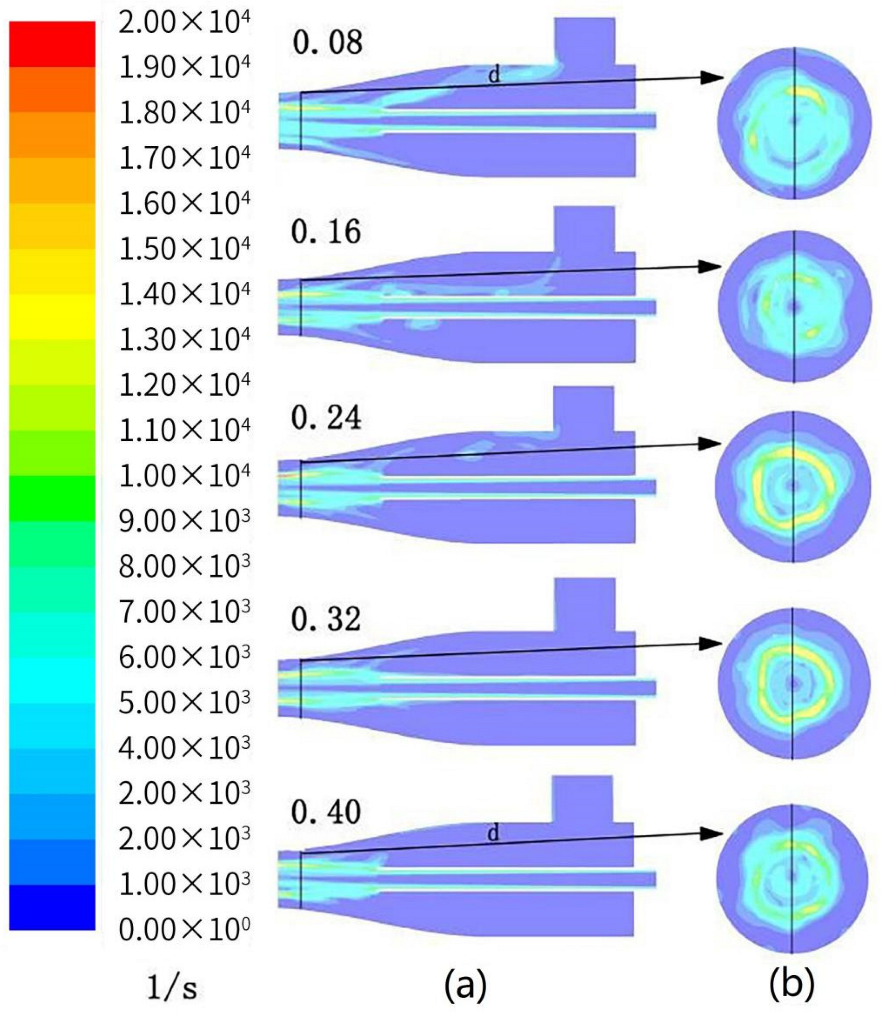
Figure 10a shows the distribution of vorticity magnitude on plane Y = 0 with different air–liquid ratios. In the inspiratory turbulent zone, Gas–Containing will increase gradually, and the original phase between the outer surface of the feeder tube and the inner surface of the nozzle will gradually be replaced by the air phase as the air–liquid ratio increases. For example, the vorticity intensity at an air–liquid ratio of 0.08 in zone “d” is much lower than that at an air–liquid ratio of 0.32 in the same zone. The distribution of vorticity magnitude on cross–section X = 0.065 m is shown in Figure 10b. With the increase in gas–liquid ratio, the vorticity intensity first increases and then decreases in the gas–water mixing zone.
When the air–liquid ratio is 0.08, the maximum vorticity intensity is 16,000 s−1. As the air–liquid ratio increases to 0.24, the maximum vorticity intensity increases to 18,000 s−1, and the gas phase is effectively mixed with the liquid phase. As the air–liquid ratio increases to 0.40, the maximum vorticity intensity decreases to 13,992 s−1.
5. Conclusions
The results of this study show that the air–liquid ratio has a significant impact on the enclosure and control of the gas–water mixing zone in the annular jet nozzle.
- For submerged annular jets, the degree of enclosure of the gas–water mixing zone in the annular jet nozzle increases with the increase in the air–liquid ratio. The main reason for this is that, as Gas–Containing increases, the degree of air–liquid mixing increases, and as a result, the core jet will be gradually dispersed in the radial direction to effectively enclose the gas–water mixing zone. As the air–liquid ratio further increases, the core jet will be further dispersed, causing water to bounce off the inner surface of the nozzle, and the degree of enclosure will remain unchanged. However, this phenomenon may cause energy dissipation, which is unfavorable for air suction;
- From the figure showing the distribution of gas–phase volume fraction, it can be observed that the increase in air–liquid ratio will result in a larger range of air–liquid mixture in the gas–water mixing zone. As the degree of dispersion of the water jet increases, the area of the gas–water mixing zone where water is bounced back will become larger, the energy of the water flow involved in enclosure will be attenuated, and more water in the tank will be suctioned into the nozzle. As a result, the area of the gas–water mixing zone where the gas phase is distributed will become smaller, and the range of the liquid phase will increase accordingly. This phenomenon is unfavorable for air suction and the effective utilization of jet energy;
- From the figure showing the distribution of turbulence intensity with different air–liquid ratios, it can be observed that as the air–liquid ratio increases, the water jet will be further dispersed, and the range of turbulence will gradually become larger. However, with the increase in the dispersion degree of the jet, the gas–liquid mixing becomes stronger, resulting in increases in turbulence intensity and vorticity intensity. As the degree of dispersion of the jet further increases, the area of the gas–water mixing zone with bounced−back water will become larger, resulting in lower local turbulence intensity and vorticity intensity. This effectively explains the mechanism whereby Gas–Containing affects the degree of enclosure of the gas–water mixing zone.
Author Contributions
Conceptualization, C.W. (Chao Wang); Data curation, C.W. (Chao Wang) and C.W. (Chuanzhen Wang); Formal analysis, C.W. (Chuanzhen Wang); Funding acquisition, C.W. (Chao Wang) and C.W. (Chuanzhen Wang); Investigation, C.W. (Chao Wang) and J.X.; Methodology, C.W. (Chao Wang); Project administration, C.W. (Chuanzhen Wang) and M.S.K.; Software, C.W. (Chao Wang) and J.X.; Supervision, J.X. and M.S.K.; Writing—original draft, C.W. (Chao Wang); Writing—review and editing, C.W. (Chao Wang) and J.X. All authors have read and agreed to the published version of the manuscript.
Funding
This work was financially supported by the research fund of the Provincial Natural Science Foundation of Anhui Province (Grant No. 1908085QE189), the Postdoctoral Research Project of Anhui (Grant No. 2019B356), the Cltivation Fund of Excellent Top—notch Talents in Colleges and Universities of Anhui Provincial Department of Education (Grant No. gxyqZD2021109), and the Provincial University Natural Science Research of Anhui (Grant No. KJ2021A0429).
Institutional Review Board Statement
Not applicable.
Informed Consent Statement
Not applicable.
Data Availability Statement
The data presented in this study are available on request from the corresponding author. The data are not publicly available due to continuous research.
Conflicts of Interest
The authors declare no conflict of interest.
References
- Ji, Y.; Song, A.; Li, C.; Cao, Y. Role of Sparger Configuration in Determining Flotation Performance under Oscillatory Air Supply. Processes 2021, 9, 638. [Google Scholar] [CrossRef]
- Santander, M.; Rodrigues, R.; Rubio, J. Modified jet flotation in oil (petroleum) emulsion/water separations. Colloids Surf. A Physicochem. Eng. Asp. 2011, 375, 237–244. [Google Scholar] [CrossRef]
- Yan, X.; Yao, Y.; Meng, S.; Zhao, S.; Wang, L.; Zhang, H.; Cao, Y. Comprehensive particle image velocimetry measurement and numerical model validations on the gas–liquid flow field in a lab-scale cyclonic flotation column. Chem. Eng. Res. Des. 2021, 174, 1–10. [Google Scholar] [CrossRef]
- Wang, X.; Shuai, Y.; Zhang, H.; Sun, J.; Yang, Y.; Huang, Z.; Jiang, B.; Liao, Z.; Wang, J.; Yang, Y. Bubble breakup in a swirl-venturi microbubble generator. Chem. Eng. J. 2021, 403, 126397. [Google Scholar] [CrossRef]
- Murai, Y.; Tasaka, Y.; Oishi, Y.; Ern, P. Bubble fragmentation dynamics in a subsonic Venturi tube for the design of a compact microbubble generator. Int. J. Multiph. Flow 2021, 139, 103645. [Google Scholar] [CrossRef]
- Li, L.; Liu, J.; Wang, L.; Yu, H. Numerical simulation of a self-absorbing microbubble generator for a cyclonic-static microbubble flotation column. Min. Sci. Technol. 2010, 20, 88–92. [Google Scholar] [CrossRef]
- Wu, M.; Yuan, S.; Song, H.; Li, X. Micro-nano bubbles production using a swirling-type venturi bubble generator. Chem. Eng. Process. Process Intensif. 2021, 170, 108697. [Google Scholar] [CrossRef]
- Foronda-Trillo, F.J.; Rodríguez-Rodríguez, J.; Gutiérrez-Montes, C.; Martínez-Bazán, C. Deformation and breakup of bubbles interacting with single vortex rings. Int. J. Multiph. Flow 2021, 142, 103734. [Google Scholar] [CrossRef]
- Li, M.; Li, W.; Hu, L. Jet formation and breakup inside highly deformed bubbles. Int. J. Heat Mass Transf. 2020, 163, 120507. [Google Scholar] [CrossRef]
- Wang, S.; Tao, X. Comparison of the adhesion kinetics between air or oily bubble and long flame coal surface in flotation. Fuel 2021, 291, 120139. [Google Scholar] [CrossRef]
- Farrokhpay, S.; Filippova, I.; Filippov, L.; Picarra, A.; Rulyov, N.; Fornasiero, D. Flotation of fine particles in the presence of combined microbubbles and conventional bubbles. Miner. Eng. 2020, 155, 106439. [Google Scholar] [CrossRef]
- Islam, M.T.; Nguyen, A.V. Effect of microturbulence on bubble-particle collision during the bubble rise in a flotation cell. Miner. Eng. 2020, 155, 106418. [Google Scholar] [CrossRef]
- Ruiz-Rus, J.; Bolaños-Jiménez, R.; Sevilla, A.; Martínez-Bazán, C. Bubble formation regimes in forced co-axial air-water jets. Int. J. Multiph. Flow 2020, 128, 103296. [Google Scholar] [CrossRef] [Green Version]
- Gutiérrez-Montes, C.; Bolaños-Jiménez, R.; Sevilla, A.; Martínez-Bazán, C. Experimental and numerical study of the periodic bubbling regime in planar co-flowing air–water sheets. Int. J. Multiph. Flow 2013, 50, 106–119. [Google Scholar] [CrossRef]
- Jamali, M.; Rostamijavanani, A.; Nouri, N.M.; Navidbakhsh, M. An experimental study of cavity and Worthington jet formations caused by a falling sphere into an oil film on water. Appl. Ocean Res. 2020, 102, 102319. [Google Scholar] [CrossRef]
- Song, H.; Chang, S.; Yu, W.; Wu, K. Experimental statistics of micrometer-sized water droplet deformation and breakup behavior in continuous air jet flow. Int. J. Multiph. Flow 2021, 135, 103529. [Google Scholar] [CrossRef]
- Deng, J.; Zhang, F.X.; Tian, Z.; Xu, W.L.; Liu, B.; Wei, W.R. Laboratory model study of the effect of aeration on axial velocity attenuation of turbulent jet flows in plunge pool. J. Hydrodyn. 2015, 27, 913–918. [Google Scholar] [CrossRef]
- Park, S.K.; Yang, H.C. Experimental investigation on mixed jet and mass transfer characteristics of horizontal aeration process. Int. J. Heat Mass Transf. 2017, 113, 544–555. [Google Scholar] [CrossRef]
- Dapelo, D.; Alberini, F.; Bridgeman, J. Euler-Lagrange CFD modelling of unconfined gas mixing in anaerobic digestion. Water Res. 2015, 85, 497–511. [Google Scholar] [CrossRef] [Green Version]
- Zhao, J.; Ning, Z.; Lv, M.; Lü, M. Large eddy simulation of the two-phase flow pattern and bubble formation process of a flow mixing nozzle under a gas–liquid mode. Fluid Dyn. Res. 2019, 51, 055510. [Google Scholar] [CrossRef]
- Wang, C.; Wang, C.; Yu, A.; Zheng, M.; Khan, M. Effect of Closure Characteristics of Annular Jet Mixed Zone on Inspiratory Performance and Bubble System. Processes 2021, 9, 1392. [Google Scholar] [CrossRef]
- Zheng, H.; Su, Y.; Zheng, L.; Ke, H. Numerical simulation of CO2 and dye separation for supercritical fluid in separator. Sep. Purif. Technol. 2020, 236, 116246. [Google Scholar] [CrossRef]
- Zolfagharnasab, M.H.; Salimi, M.; Aghanajafi, C. Application of non-pressure-based coupled procedures for the solution of heat and mass transfer for the incompressible fluid flow phenomenon. Int. J. Heat Mass Transf. 2021, 181, 121851. [Google Scholar] [CrossRef]
- Almitani, K.H.; Alzaed, A.; Alahmadi, A.; Sharifpur, M.; Momin, M. The influence of the geometric shape of the symmetrical twisted turbulator on the performance of parabolic solar collector having hybrid nanofluid: Numerical approach using two-phase model. Sustain. Energy Technol. Assess. 2022, 51, 101882. [Google Scholar] [CrossRef]
- Garoosi, F.; Hooman, K. Numerical simulation of multiphase flows using an enhanced Volume-of-Fluid (VOF) method. Int. J. Mech. Sci. 2021, 215, 106956. [Google Scholar] [CrossRef]
- Garoosi, F.; Merabtene, T.; Mahdi, T.-F. Numerical simulation of merging of two rising bubbles with different densities and diameters using an enhanced Volume-of-Fluid (VOF) model. Ocean Eng. 2022, 247, 110711. [Google Scholar] [CrossRef]
- Cerqueira, R.F.; Paladino, E.E.; Evrard, F.; Denner, F.; van Wachem, B. Multiscale modeling and validation of the flow around Taylor bubbles surrounded with small dispersed bubbles using a coupled VOF-DBM approach. Int. J. Multiph. Flow 2021, 141, 103673. [Google Scholar] [CrossRef]
Figure 1.
Experimental test system. (a) Diagram of test system; (b) Structural diagram of annular jet nozzle. (c) Sectional view of annular jet nozzle.
Figure 1.
Experimental test system. (a) Diagram of test system; (b) Structural diagram of annular jet nozzle. (c) Sectional view of annular jet nozzle.

Figure 2.
Meshing diagram of nozzle and observation tank. (a) Combined meshing diagram of observation tank and annular jet nozzle. (b) Meshing diagram of annular jet nozzle. (c) Cross– section mesh of the annular nozzle on X = 0.065 m.
Figure 2.
Meshing diagram of nozzle and observation tank. (a) Combined meshing diagram of observation tank and annular jet nozzle. (b) Meshing diagram of annular jet nozzle. (c) Cross– section mesh of the annular nozzle on X = 0.065 m.

Figure 3.
Radial velocity error under different grid density.

Figure 4.
Comparison of numerical model and experiment.

Figure 5.
Velocity vector diagram of gas–water mixing zone in nozzle with different air–liquid ratios.
Figure 5.
Velocity vector diagram of gas–water mixing zone in nozzle with different air–liquid ratios.

Figure 6.
Velocity change curve of gas–water mixing zone with different gas–liquid ratios.

Figure 7.
Distribution of gas volume fraction with different gas–liquid ratios. (a) Distribution of gas–phase volume fractions on plane Y = 0. (b) Distribution of gas–phase volume fractions on cross–section X = 0.065 m.
Figure 7.
Distribution of gas volume fraction with different gas–liquid ratios. (a) Distribution of gas–phase volume fractions on plane Y = 0. (b) Distribution of gas–phase volume fractions on cross–section X = 0.065 m.

Figure 8.
Distribution diagram of turbulence intensity with different gas–liquid ratios. (a) Distribution of turbulence intensity in the annular jet nozzle on plane Y = 0. (b) Distribution curves of the values of turbulence intensity at the intersection between plane Y = 0 and cross–section X = 0.065 m.

Figure 9.
Schematic diagram of turbulence changes with different gas–liquid ratios.

Figure 10.
Distribution diagram of vorticity magnitude with different gas–liquid ratios. (a) Distribution of vorticity magnitude on plane Y = 0. (b) Distribution of vorticity magnitude on cross–section X = 0.065 m.
Figure 10.
Distribution diagram of vorticity magnitude with different gas–liquid ratios. (a) Distribution of vorticity magnitude on plane Y = 0. (b) Distribution of vorticity magnitude on cross–section X = 0.065 m.


Table 1.
Numerical calculation design and the results.
| m3/h MPa | 20 mm (EXP) | 20 mm (CFD) | ||||||||||||
|---|---|---|---|---|---|---|---|---|---|---|---|---|---|---|
| 0.06 | 0.08 | 0.10 | 0.12 | 0.14 | 0.16 | 0.18 | 0.06 | 0.08 | 0.10 | 0.12 | 0.14 | 0.16 | 0.18 | |
| 0.079 | 0.124 | 0.168 | 0.233 | 0.304 | 0.324 | 0.336 | 0.086 | 0.135 | 0.184 | 0.253 | 0.333 | 0.352 | 0.375 | |
| 0.408 | 0.508 | 0.561 | 0.615 | 0.674 | 0.709 | 0.789 | 0.423 | 0.527 | 0.576 | 0.638 | 0.699 | 0.735 | 0.808 | |
| 0.194 | 0.244 | 0.299 | 0.379 | 0.451 | 0.457 | 0.426 | 0.203 | 0.256 | 0.320 | 0.397 | 0.477 | 0.479 | 0.464 | |
Publisher’s Note: MDPI stays neutral with regard to jurisdictional claims in published maps and institutional affiliations. |
© 2022 by the authors. Licensee MDPI, Basel, Switzerland. This article is an open access article distributed under the terms and conditions of the Creative Commons Attribution (CC BY) license (https://creativecommons.org/licenses/by/4.0/).
Share and Cite
MDPI and ACS Style
Wang, C.; Wang, C.; Xie, J.; Khan, M.S. Influence Mechanism of Gas–Containing Characteristics of Annulus Submerged Jets on Sealing Degree of Mixing Zone. Processes 2022, 10, 593. https://0-doi-org.brum.beds.ac.uk/10.3390/pr10030593
AMA Style
Wang C, Wang C, Xie J, Khan MS. Influence Mechanism of Gas–Containing Characteristics of Annulus Submerged Jets on Sealing Degree of Mixing Zone. Processes. 2022; 10(3):593. https://0-doi-org.brum.beds.ac.uk/10.3390/pr10030593
Chicago/Turabian StyleWang, Chao, Chuanzhen Wang, Jun Xie, and Md Shakhaoath Khan. 2022. "Influence Mechanism of Gas–Containing Characteristics of Annulus Submerged Jets on Sealing Degree of Mixing Zone" Processes 10, no. 3: 593. https://0-doi-org.brum.beds.ac.uk/10.3390/pr10030593
Note that from the first issue of 2016, this journal uses article numbers instead of page numbers. See further details here.