A Feedback Control Strategy for a Fed-Batch Monoclonal Antibody Production Process Utilising Infrequent and Irregular Sampled Measurements

Abstract

The ability to take non-invasive Raman measurements presents a unique opportunity to use one Raman probe across multiple vessels in parallel, reducing costs but making measurements infrequent. Under these conditions, infrequent and irregular feedback signals can result in poor closed-loop control performance. This study addressed the issue of infrequent and irregular Raman measurements using a linear dynamic model developed from interpolated data to predict more frequent measurements of the controlled variable. The simulated monoclonal antibody production was sampled hourly with white noise added to the simulated glucose concentration to replicate real Raman measurements. The hourly samples were interpolated into 15 min intervals and a linear dynamic model was developed to predict the glucose concentration at 15 min intervals. These predicted values were then used in a feedback control loop by using model predictive control or a conventional proportional and integral controller to control the glucose concentration at 15 min sampling intervals. For setpoint tracking, the model predictive control reduced the integral of absolute errors to 14,600 from 15,900 (with a 1 h sampling time) or 8.2% reduction. With adaptive model predictive control, the integral of absolute errors was reduced from 14,500 (1 h sampling time) to 14,200 for setpoint tracking and from 13,500 (1 h sampling time) to 13,300 for disturbance rejection. A final comparison demonstrated that the proposed method can also cope with random variations in the sampling time.

1. Introduction

The rise in biopharmaceuticals in recent years has seen the fermentation process applied in the production of therapeutic proteins including monoclonal antibodies (mAbs) and some vaccines [1]. As well as their use in oncology, several companies are currently developing mAbs to be used in the treatment of COVID-19 patients [2]. Where used in medicine, the product quality must be ensured for the treatment to have the desired effect, and more importantly, to avoid further harm [3].

To ensure product quality, rapid and reliable fermentation control is essential. Even small disturbances in fermenter conditions will result in a lag phase as the cells adjust, and in more extreme cases, it can lead to irreversible cell death [4]. Despite this, process control in the pharmaceutical industry has historically lagged behind its chemical manufacturing counterpart. This is often attributed to a lack of suitable real-time measurement techniques, referred to as process analytical technologies (PATs) [5,6,7]. The issue was addressed by the U.S. Food and Drug Administration (FDA) in their 2004 report, which encouraged the pharmaceutical industry to adopt a quality by design (QbD) approach. This means measuring the critical process parameters (CPPs) in real-time and maintaining them to ensure product quality, as opposed to testing the product quality after the fact [8].

The guidance issued by the FDA led to renewed interest in the development of PATs, particularly spectrometry. When paired with a multivariate method, spectrometry can be used for real-time measurements of multiple CPPs [9]. In addition, measurements can be taken non-invasively through a glass window, removing the risk of contamination [2]. Of the spectroscopic methods considered, Raman is generally preferred as it does not suffer interference from water, and therefore has a higher signal-to-noise ratio (SNR) [5]. Several recent case studies have shown its successful application for real-time fermentation measurements [10,11].

Where Raman spectroscopy is used as the PAT, the frequency of measurements is limited by a long exposure time, and sampling intervals are in the order of minutes rather than seconds [8,9]. Furthermore, a Raman probe is often used across a number of fermenters for cost saving. Under these conditions, infrequent and irregular feedback signals can cause poor feedback control performance. When proportional integral derivative (PID) control is used in such cases, the response can either be too oscillatory or undesirably sluggish [12]. The ability to take Raman measurements non-invasively presents a unique opportunity to use one probe across multiple vessels in parallel and reduce the costs. Under these conditions, the frequent measurements used by Craven et al. [5] and Rodrigues et al. [13] are not possible, and the control performance will suffer as a result.

Some approaches have been reported in the literature to cope with infrequent measurements in feedback control, but very few have dealt with batch process control. Wang and Georgakis [14] proposed a dynamic response surface methodology approach for the identification of Hammerstein–Wiener models from infrequent measurements in the batch processes. The identified Hammerstein–Wiener model was then used in a model predictive control (MPC) framework and better performance than linear MPC was obtained. However, the construction of such a model needs the design of experiments, which would perturb the production process. Other approaches involve inferential estimation or inferential control using the extended Kalman filter [15], dual rate modelling [16], or unscented Kalman filter [17], where accurate state space modelling is required. Furthermore, irregular sampling intervals are not considered in these approaches.

This paper proposes using interpolation on infrequent (and irregular sampled) measurements and then constructing a linear autoregressive with exogenous input (ARX) model to estimate the controlled variable at a much shorter interval. These estimations are then used in feedback control. The motivation of the proposed approach is to address the practical situations where a Raman probe is used across a number of fermenters or reactors for cost saving. In such cases, the Raman measurement is mainly for product quality monitoring. With the method proposed in this paper, these infrequent (and irregular sampled) Raman measurements can be used in closed-loop control. This ARX model can be updated each time when a new Raman sample is available. The novelty of the proposed approach is that it does not rely on accurate state space modelling and its implementation is straightforward. Furthermore, it can also handle irregular samples, as demonstrated in this paper.

A simulation of a fed-batch monoclonal antibody production process was created in MATLAB/Simulink and white noise was added to the hourly samples to represent the real Raman measurements. The noisy measurements were then filtered and interpolated into 15 min intervals, and these values were used to develop a linear ARX model for use in the MPC algorithm. The effect of ARX prediction was shown through a comparison of the MPC performance with and without interpolation. In both cases, the factorial design method described by Box et al. [18] was used to find the tuning parameters that minimised the integral absolute error (IAE).

The rest of the paper is organised as follows. Section 2 presents the materials and methods, where the reactor simulation and scale up, data sampling and interpolation, ARX model development and adaptation, and control algorithms are detailed. Section 3 presents the results and discussions. Some concluding remarks are given in Section 4.

2. Materials and Methods

2.1. Reactor Simulation and Scale-Up

A model of mAb production was created using Equations (1)–(17). Taken from [19], the equations were solved in MATLAB/Simulink using ODE45 and the constant values in

Table 1. The constants and initial conditions used in replicating the results in [19].

Constants
Parameter	Value	Unit
KG,GLC	14.655	mM
KG,GLU	0.534	mM
KI,AMM	4.682	mM
KI,LAC	55.562	mM
KLAG	10.624	n/a
KLYS	0.0026	h−1
KMET	5.853	mM
KQ,GLN	0.0013	mM
mMAB	4.02 × 10−11	Mg (mM)−1 cell−1 h−2
QMAX, GLN	6.99517 × 10−9	mM cell−1 h−1
YAMM,GLN	1.21	mM (mM)−1
YLAC,GLC	1.253	mM (mM)−1
YX,GLC	163,894	Cells mM−1
YX,GLU	1.20763 × 106	Cells mM−1
YX,MAB	577,914	mg L−1 cell−1
$\mathsf{\mu }$d,max	0.188	h−1
$\mathsf{\mu }$MAX,GLC	0.073	h−1
$\mathsf{\mu }$MAX,GLU	0.454	h−1
Initial conditions
V0	200	mL
XV,0	2 × 105	Cells (mL)−1
XD,0	1 × 104	Cells (mL)−1
[mAb]0	5.65	mg (L)−1
[GLC]0	20	mM
[GLU]0	0.8	mM

. A trial simulation replicated the results presented by Kiparissises et al. [19], confirming that the simulation was successful.

$$\mathsf{\mu }={\mathsf{\mu }}_{\mathrm{GLC}}+{\mathsf{\mu }}_{\mathrm{GLU}}$$

(1)

$${\mathsf{\mu }}_{\mathrm{GLU}}={\mathsf{\mu }}_{\mathrm{MAX},\mathrm{GLU},\mathsf{\varphi }}\frac{{\left[\mathrm{GLU}\right]}^2}{{\mathrm{K}}_{\mathrm{G},\mathrm{GLU}}^2+{[\mathrm{GLU}]}^2}$$

(2)

$${\mathsf{\mu }}_{\mathrm{GLC}}=\left(1-{\mathrm{Q}}_{\mathrm{met}}\right){\mathsf{\mu }}_{\mathrm{MAX},\mathrm{GLC}}\frac{{\left[\mathrm{GLC}\right]}^2}{{\mathrm{K}}_{\mathrm{G},\mathrm{GLC}}^2+{[\mathrm{GLC}]}^2}\frac{1}{1+{\mathrm{K}}_{\mathrm{I},\mathrm{AMM}}\left[\mathrm{AMM}\right]}$$

(3)

$${\mathrm{Q}}_{\mathrm{MET}}=\frac{\left[\mathrm{GLU}\right]}{{\mathrm{K}}_{\mathrm{MET}}+\left[\mathrm{GLU}\right]}$$

(4)

$${\mathrm{Q}}_{\mathrm{LAC}}={\mathrm{Q}}_{\mathrm{GLC}}{\mathrm{Y}}_{\mathrm{LAC},\mathrm{GLC}}$$

(5)

$${\mathrm{Q}}_{\mathrm{GLN}}=\left(1-{\mathrm{Q}}_{\mathrm{MET}}\right){\mathrm{Q}}_{\mathrm{MAX},\mathrm{GLN}}\frac{{\left[\mathrm{GLN}\right]}^2}{{\mathrm{K}}_{\mathrm{Q},\mathrm{GLN}}^2+{[\mathrm{GLN}]}^2}$$

(6)

$${\mathsf{\mu }}_{\mathrm{d}}=\frac{{\mathsf{\mu }}_{\mathrm{d},\max }}{1+{({\mathrm{K}}_{\mathrm{I},\mathrm{lac}}/\mathrm{LAC})}^2}$$

(7)

$${\mathrm{Q}}_{\mathrm{GLC}}=\frac{{\mathsf{\mu }}_{\mathrm{GLC}}}{{\mathrm{Y}}_{\mathrm{x},\mathrm{GLC}}}$$

(8)

$$\mathrm{For}\left[\mathrm{GLU}\right]<0,{\mathrm{Q}}_{\mathrm{GLU}}=0;[\mathrm{GLU}]>0,{\mathrm{Q}}_{\mathrm{GLU}}=\frac{\mathsf{\mu }}{{\mathrm{Y}}_{\mathrm{X},\mathrm{GLU}}}$$

(9)

$$\frac{\mathrm{d}\left(\left[\mathrm{LAC}\right]\mathrm{V}\right)}{\mathrm{dt}}={\mathrm{Q}}_{\mathrm{LAC}}{\mathrm{X}}_{\mathrm{v}}\mathrm{V}-{\mathrm{F}}_{\mathrm{OUT}}\left[\mathrm{LAC}\right]$$

(10)

$$\frac{\mathrm{d}\left[\mathrm{GLN}\right]}{\mathrm{dt}}={\mathrm{Q}}_{\mathrm{GLU}}{\mathrm{X}}_{\mathrm{v}}-{\mathrm{Q}}_{\mathrm{GLN}}{\mathrm{X}}_{\mathrm{v}}$$

(11)

$$\frac{\mathrm{d}\left(\left[\mathrm{mAb}\right]\mathrm{V}\right)}{\mathrm{dt}}=\left(\frac{{\mathsf{\mu }}_{\mathrm{GLU}}}{{\mathrm{Y}}_{\mathrm{x},\mathrm{mAb}}}+{\mathrm{m}}_{\mathrm{mAb}}\frac{\left[\mathrm{GLC}\right]}{\mathsf{\mu }}\right){\mathrm{X}}_{\mathrm{v}}\mathrm{V}-{\mathrm{F}}_{\mathrm{OUT}}\left[\mathrm{mAb}\right]$$

(12)

$$\frac{\mathrm{d}\left({\mathrm{VX}}_{\mathrm{v}}\right)}{\mathrm{dt}}=\left(\mathsf{\mu }-{\mathsf{\mu }}_{\mathrm{d}}\right){\mathrm{X}}_{\mathrm{v}}\mathrm{V}-{\mathrm{F}}_{\mathrm{out}}{\mathrm{X}}_{\mathrm{v}}$$

(13)

$$\frac{\mathrm{d}\left({\mathrm{VX}}_{\mathrm{D}}\right)}{\mathrm{dt}}={\mathsf{\mu }}_{\mathrm{d}}{\mathrm{X}}_{\mathrm{v}}\mathrm{V}-{\mathrm{k}}_{\mathrm{lys}}{\mathrm{X}}_{\mathrm{D}}\mathrm{V}-{\mathrm{F}}_{\mathrm{out}}{\mathrm{X}}_{\mathrm{D}}$$

(14)

$$\frac{\mathrm{d}\left(\left[\mathrm{GLC}\right]\mathrm{V}\right)}{\mathrm{dt}}=-{\mathrm{Q}}_{\mathrm{GLC}}{\mathrm{X}}_{\mathrm{v}}\mathrm{V}+{\mathrm{F}}_{\mathrm{in}}{[\mathrm{GLC}]}_{\mathrm{IN}}-{\mathrm{F}}_{\mathrm{out}}\left[\mathrm{GLC}\right]$$

(15)

$$\frac{\mathrm{d}\left(\left[\mathrm{GLU}\right]\mathrm{V}\right)}{\mathrm{dt}}=-{\mathrm{Q}}_{\mathrm{GLU}}{\mathrm{X}}_{\mathrm{v}}\mathrm{V}+{\mathrm{F}}_{\mathrm{in}}{[\mathrm{GLU}]}_{\mathrm{in}}-{\mathrm{F}}_{\mathrm{out}}\left[\mathrm{GLU}\right]$$

(16)

$$\frac{\mathrm{dV}}{\mathrm{dt}}={\mathrm{F}}_{\mathrm{in}}-{\mathrm{F}}_{\mathrm{out}}$$

(17)

In the above equations, μ is the growth rate (h⁻¹); ${\mathsf{\mu }}_{\mathrm{d}}$ is the death rate (h⁻¹); ${\mathsf{\mu }}_{\mathrm{glc}}$ and ${\mathsf{\mu }}_{\mathrm{glu}}$ are the growth rates from glucose and glutamate consumption (h⁻¹), respectively; AMM, GLC, GLN, GLU, and LAC represent ammonia, glucose, glutamine, glutamate, and lactate, respectively, [ ] represents the concentration (mM); Q represents the specific uptake rate (m Mh⁻¹); V is the culture volume (L); F_in and F_out are the input and output volumetric flow rate (L/h). The parameters of the model are given in Table 1.

The results presented by in [19] were validated using a lab-scale experiment where pulses in the feed flowrate varied between 0.5–4 mL h⁻¹. A controller design on this scale would be redundant, and instead, a scaled-up version of the simulation to represent the production scale was considered.

In the following study, a total reactor volume of 2500 L [20] was assumed to have a starting volume of 70% [21] and a maximum working volume of 80% [22]. The scaled-up simulation assumed that the reaction kinetics and initial conditions remained the same, with the exception of the feed concentration of glucose and glutamine, which were increased to reflect a practical scale-up and to prevent excessive feed flowrates [20]. Concentrations of 555 mM and 200 mM for glucose and glutamine, respectively, were taken from Sigma Aldrich to reflect those available on the market.

2.2. Imitation of Raman Sampling

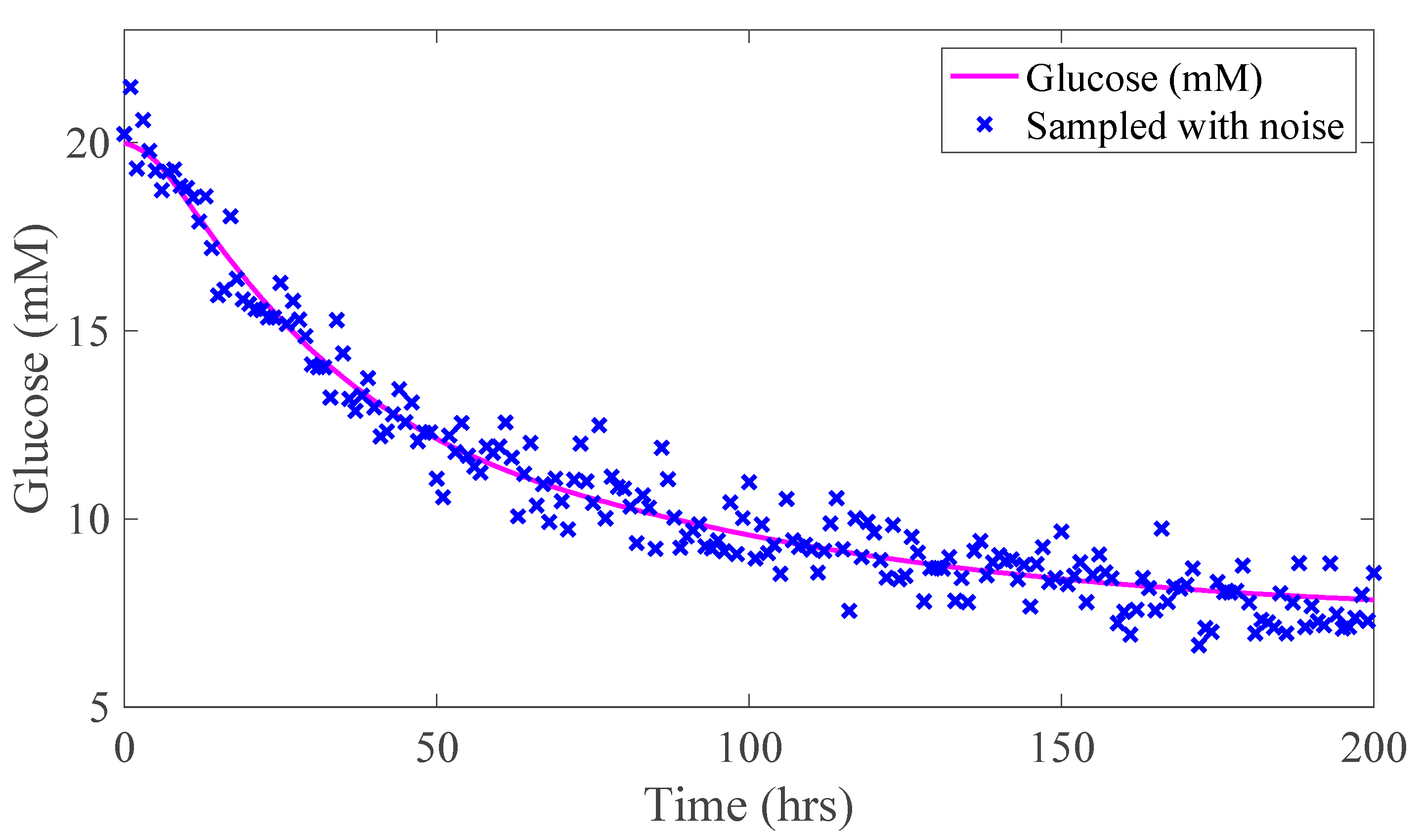
When Raman spectroscopy is used to measure glucose concentration, it is unreasonable to expect measurements to be without noise. Instead, white noise with a SNR of 25 [5] was added to the hourly samples taken from the simulation. The effect of this noise on the control variable, glucose concentration, is shown in Figure 1.

2.3. ARX Model Development

MPC requires a dynamic model of the process, which can be used to optimize future values of the control variable. In this case, the linear ARX model, shown in Equation (18) [23], was used.

$$A\left(z^{-1}\right)y\left(t\right)=B\left(z^{-1}\right) u\left(t-1\right)+\epsilon \left(t\right)$$

(18)

where

$$(z^{-1})=1+a_1{z}^{-1}+a_2{z}^{-2}+\cdots +a_{Na}{z}^{-Na}$$

and

$$B(z^{-1})=b_1{z}^{-1}+b_2{z}^{-2}+\cdots +b_{Nb}{z}^{-Nb}$$

In the above equation, y(t) is the control variable, glucose concentration; u(t) is the manipulated variable, feed flowrate; $\epsilon \left(t\right)$ is an exogeneous input; N_a and N_b are the orders of regressors $A(z^{-1})$ and $B(z^{-1}),$ respectively; [a₁, a₂ …] and [b₁, b₂ …] are coefficients of regressors $A(z^{-1})$ and $B(z^{-1})$ respectively, chosen so that the current output, y(t), is a weighted average of previous values.

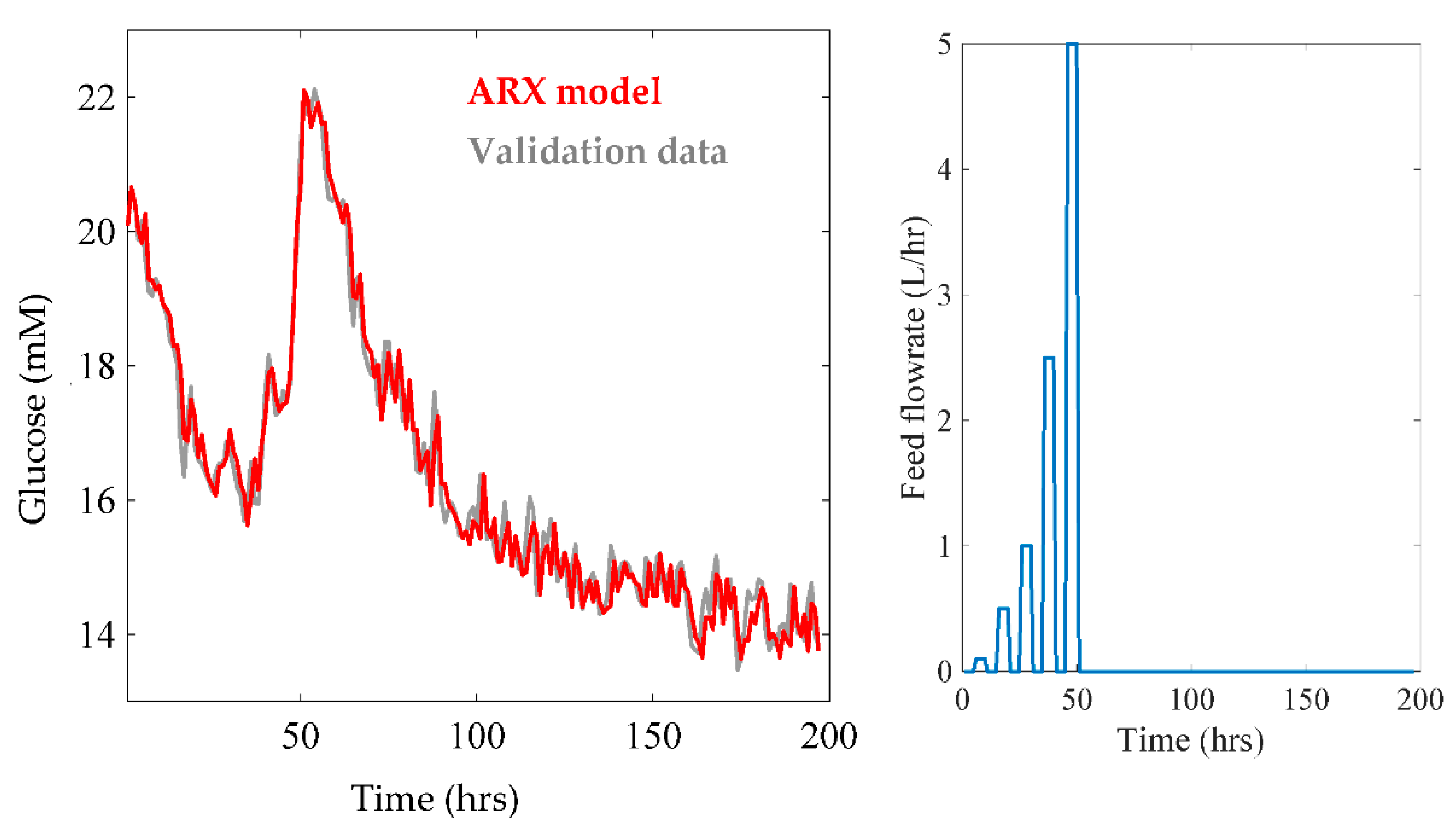
The coefficients [a₁, a₂ …] and [b₁, b₂ …] were estimated using the ‘arx’ function in MATLAB, which uses the least squares method to find values of a and b, which minimize the one step ahead prediction error. The training data, given in Figure 2, were produced using feed flowrates between 0.1 and 5 L h⁻¹.

The simulated glucose concentration measurement with noise was smoothed to further remove noise. The smoothed data were interpolated into 15 min intervals, and these interpolated data were used to develop a secondary ARX model, which was used in predicting and controlling the glucose concentration at a shorter sampling interval. The final model order was decided through a comparison of the control performance for setpoint tracking and disturbance rejection, as discussed in the Results Section.

2.4. Online Adaptation of the ARX Model

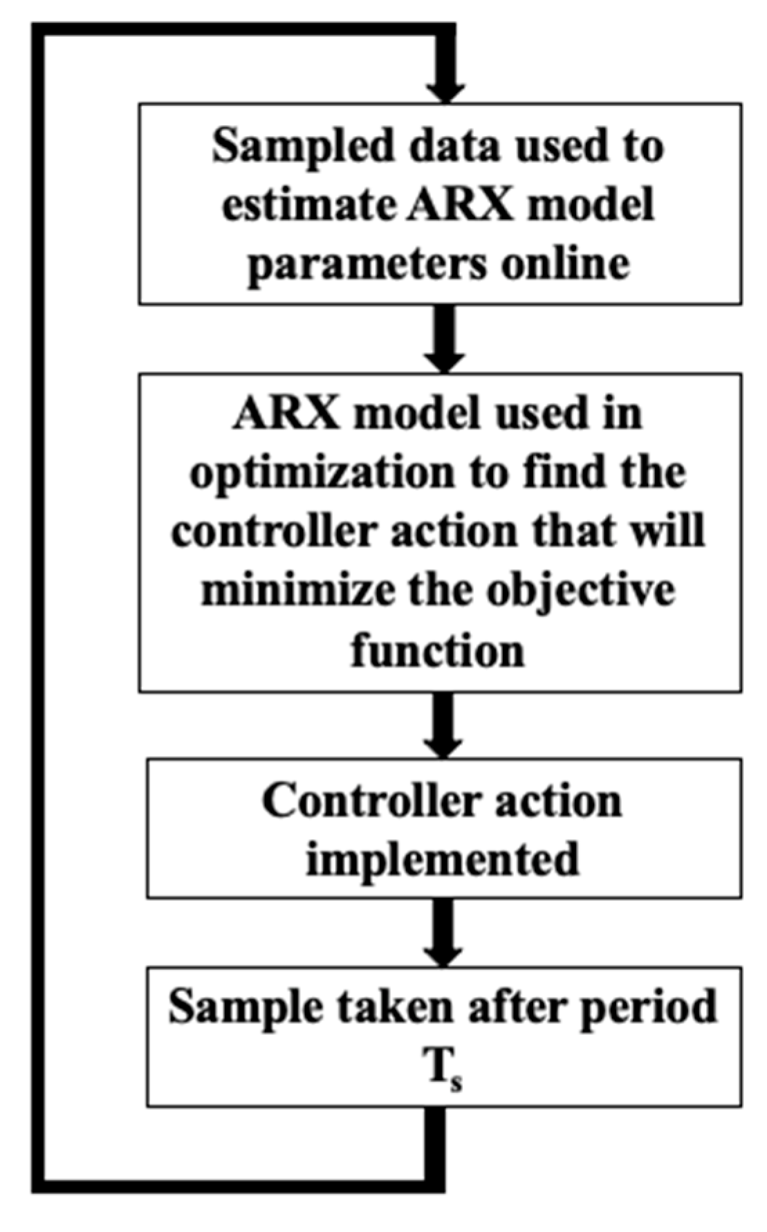
In adaptive configuration, the ARX model parameters were re-estimated at each sampling interval, as shown in Figure 3. The recursive estimation was carried out using the ‘recursive polynomial model estimator block’ in Simulink, with a forgetting factor algorithm. The algorithm, shown in Equation (19), was used to discount old estimates of the ARX parameters across a given number of samples (T_o).

$$T_o=\frac{1}{1-\delta }$$

(19)

where $T_o$ is the sample number and $\delta$ is the forgetting factor. The value of $\delta$ can be specified within the Simulink block. It is recommended that $\delta$ < 1 be used when the ARX parameters are time varying. Otherwise, a value of 1 can be used to create a recursive estimator that accounts for all of the previous values (i.e., no forgetting).

2.5. The Feedback Controllers

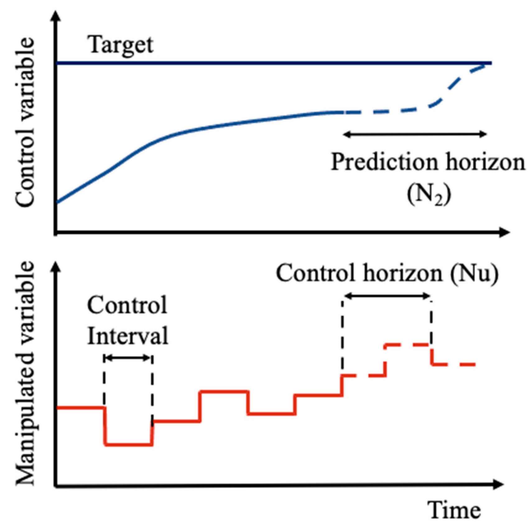
The MPC uses a dynamic model of the process to predict future outputs (y) for a given change in the manipulated variable (u). The model was used in an optimisation problem at each sampling interval to find the controller actions that will minimize the objective function (J) across a prediction horizon, N₂, as shown in Figure 4 [24]. The first controller action was then implemented, and the process repeated at each sampling interval.

Early implementation of MPC used linear models and was widely applied in the petrochemical industry [24]. However, when applied to processes such as fermentation, the same MPC algorithms had limited success [25]. This is because the linear models used in these algorithms cannot accurately represent the non-linearities of fermentation. Instead, more recent studies have focused on the use of non-linear models [24].

Among others, non-linear MPC (NMPC) has been applied in fermentation control by Craven et al. [5], who used Raman spectrometry to measure the glucose concentration with a sample time of 6 min. Despite some success in research, NMPC is yet to be widely applied in industry. This is because, unlike linear models, which have a clear global minima in optimisation, non-linear dynamic models create an optimisation problem with many local minima. Iterative solutions are required to find the global minima, making the optimisation slow and computationally expensive [26].

Online adaptation of a linear model can be used in some cases to control a non-linear process with reduced computational expense. Known as adaptive MPC, this method assumes that a non-linear process can be approximated by a linear model for a small time interval. By updating the linear model parameters at each sample interval, the non-linear process is represented as a series of linear models [13].

Where online adaptation of the model is required, generalised predictive control (GPC), created by Clarke et al. [23], is generally the preferred algorithm. GPC uses a variation of the linear ARX model, which has few parameters and is therefore easily adapted online [18]. Adaptive-GPC has been applied in fermentation control by Rodrigues et al. [16], who initially used a sampling time of 6 min. When this was later increased to 12 min, Rodrigues et al. [13] remarked on how longer sampling intervals caused quick deterioration of the MPC performance.

The model predictive control in the form of GPC [23] was used here to control the glucose concentration in the reactor. The adaptive MPC shown in Figure 3 was also implemented. For the purpose of comparison, a traditional PID controller was also used.

The derivative action of a PID controller gives a fast response to small changes in the manipulated variable. In noisy systems such as the one considered here, this can cause excessive noise in the manipulated variable [27]. As such, the discrete PI controller shown in Equation (20) [28] was used instead.

$$\frac{u\left(s\right)}{e\left(s\right)}=k_c+\frac{k_c}{T_I}(\frac{1}{1-s^{-1}})$$

(20)

where s is the Laplace operator, e(s) is the control error, k_c is the controller gain, and T_i is the integral time constant.

Controller parameters (k_c, T_i) were found by the conversion of the second-order ARX model to a continuous time transfer function using the ‘c2d’ function in MATLAB. Through a comparison of the resulting transfer function with Equation (21), its parameters were fully defined and used in Equations (22) and (23) [29].

$$G_P\left(s\right)=\frac{K_m\left(1+T_{m3}s\right)e^{-s{\tau }_m}}{T_{ml}{}^2{s}^2+2{\xi }_m{T}_{ml}s+1}$$

(21)

$$K_c=\frac{2{\xi }_m{T}_{ml}+0.5{\tau }_m}{k_m\left(2\lambda +{\tau }_m\right)}$$

(22)

$$T_i=2{\xi }_m{T}_{ml}+0.5{\tau }_m$$

(23)

where K_m is the gain of the process model, $T_{ml}$ and $T_{m3}$ are the time constants associated with the lag and lead terms of the process model respectively, ${\tau }_m$ is the time delay (min), ${\xi }_m$ is the damping factor, and $\lambda$ is a robustness parameter of a compensated system.

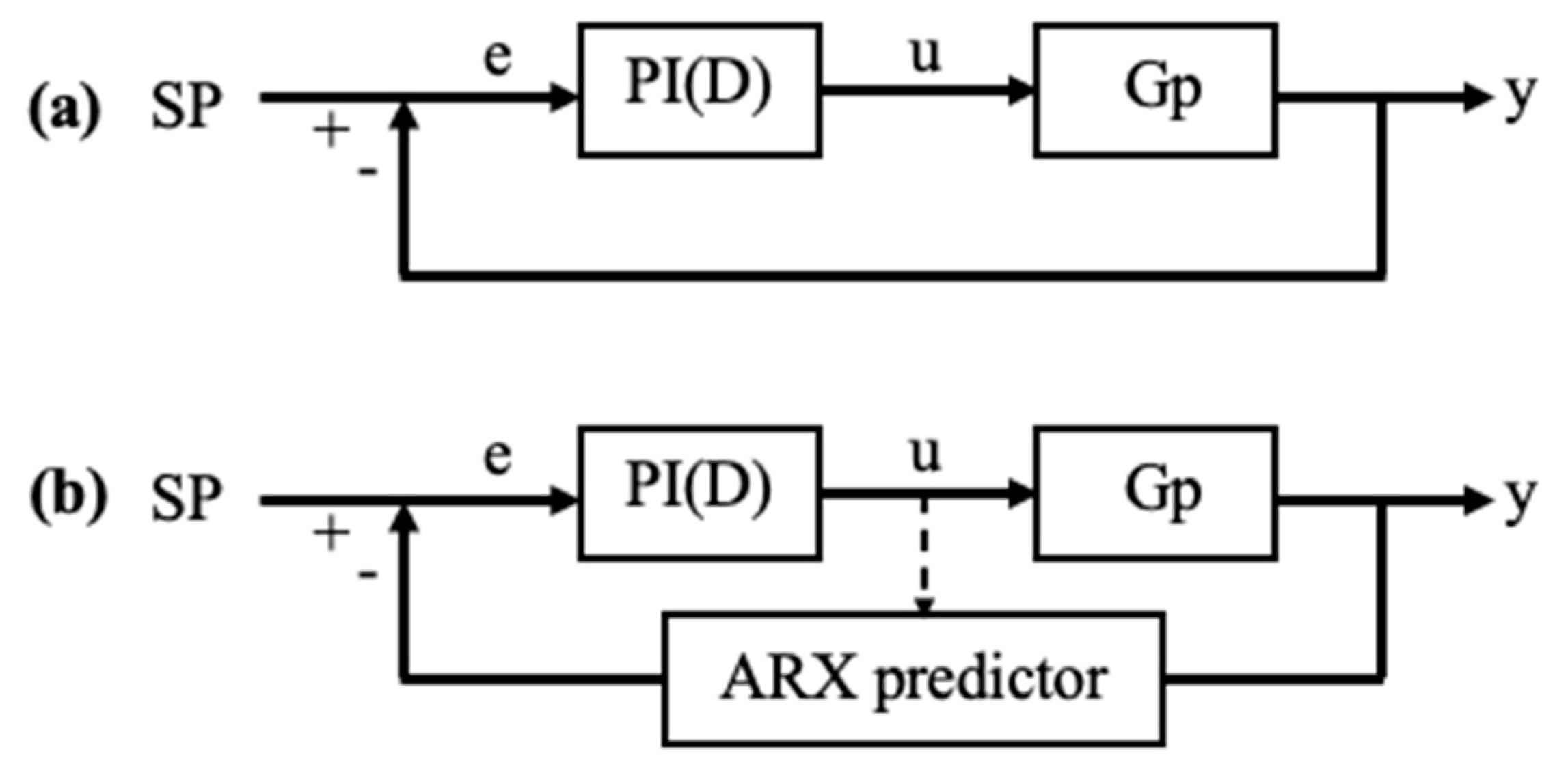
The PI or GPC controller was then implemented in one of the two configurations shown in Figure 5. The first (a) operates as a standard PI or GPC control loop, where error calculations are carried out at each sampling interval. The second, (b), uses an ARX model to predict more frequent values of y within the same sampling interval to give more frequent feedback errors.

2.6. Irregular Sampling

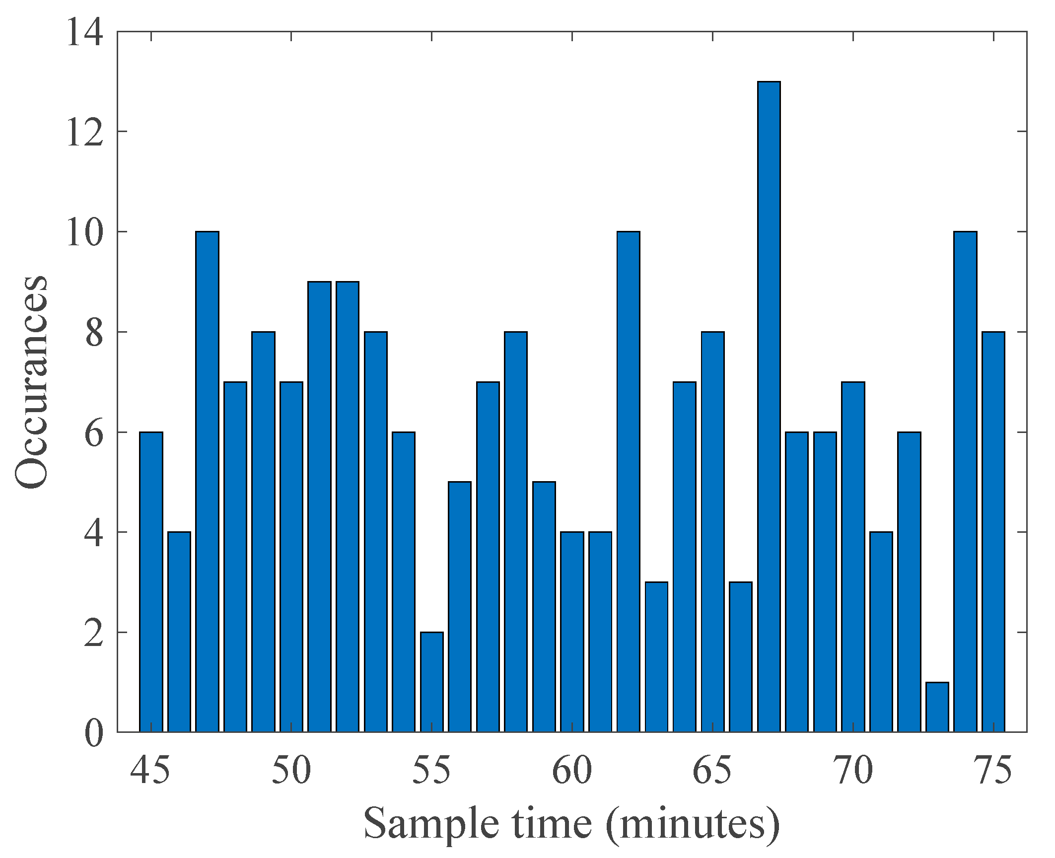
When a Raman probe is used across multiple vessels in parallel, it is unlikely that the sampling time would be consistent. To observe the effects of this on the controller performance, a simulation was created in which the sampling time was varied randomly between two limits. The sample intervals were found using a random number generator in MATLAB (see Figure 6) and used to trigger the Simulink subsystem where the relevant controller calculations were carried out. When irregular sampling is used, conventional filtering is not appropriate. Instead, measurements were interpolated into 15 min intervals prior to smoothing. Note that this method was not used in the controller development, only in the final robustness analysis.

2.7. Controller Performance Criteria

The performance of each controller was compared by looking at the IAE, integral squared error (ISE), and the control effort (Δu^TΔu), as shown in Equations (24)–(26) [27].

$$IAE={{\displaystyle \int }}_0^t\left|e\left(t\right)\right|$$

(24)

$$ISE={{\displaystyle \int }}_0^{t}e{\left(t\right)}^2$$

(25)

$$\Delta u^T\Delta u={\displaystyle \sum }_0^t{(u\left(t\right)-u\left(t-1\right))}^2$$

(26)

The IAE weights each error equally and is widely used to compare the overall performance of controllers. Conversely, the square in ISE means that larger control errors are weighted more heavily [27], making it useful for comparisons to setpoint tracking and disturbance rejections.

Finally, the work by the manipulated variable was checked to make sure that it was not excessive. Rapid changes in the feed flowrate will cause wear on a valve over time, which will need more frequent replacements as a result. As well as looking at Δu^TΔu, any large and sudden changes should be noted, as these may not be achievable in practice.

3. Results and Discussion

3.1. MPC Controller Design

3.1.1. Non-Adaptive MPC

To start, a third-order ARX model was assumed to be appropriate, and its parameters were found using the ‘arx’ function as previously described. The resulting parameters for a glucose sampling interval of 60 min were a₁ = −0.975, a₂ = 0.444, a₃ = −0.461, b₁ = 1.31 × 10⁻⁴, b₂ = 9.92 × 10⁻⁵, and b₃ = 6.64 × 10⁻⁵.

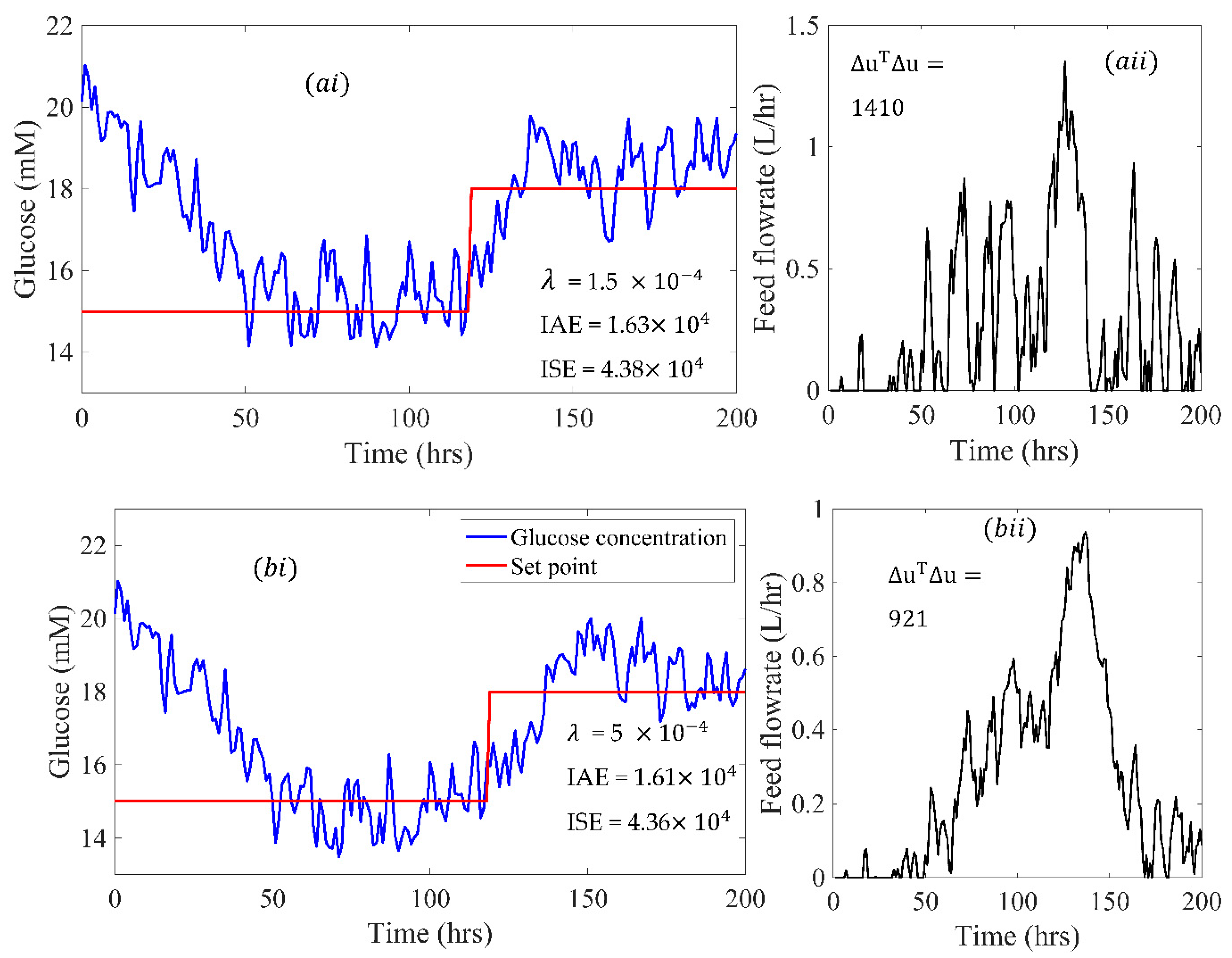
Controller tuning was carried out using the factorial design method described by Box et al. [16] and previously used by Rodrigues et al. [13]. This is a simple, though thorough, tuning method where every parameter is given a range of possible values, and then the performance of all possible combinations of these parameters compared. The minimum and maximum values, given in

Table 2. The minimum and maximum tuning parameters considered in the factorial design.

	λ	N2	Nu
Min	0.1 × 10−4	5	1
Max	6 × 10−4	15	3

, were found through trial and error, and then compared for the step change in setpoint shown in Figure 7.

Figure 7 shows the effect of λ on the controller performance. When a small value of λ is chosen, the response is rapid, but the noise in the manipulated variable is high. Increasing λ restricts the changes in the feed flowrate, as shown in Figure 7bii, but the response becomes sluggish with a significant overshoot. Similar observations have been made by Craven et al. [5]. However, where these results differ is that a small value of λ in this case resulted in the excess feeding of glucose in the final 50 h. This could be caused by the slowing of the reaction with time, which cannot be accounted for with a non-adaptive and linear ARX model. It can be seen that the response shown in Figure 7 qualitatively matched those reported in [5], which was on a mammalian cell fed-batch process but with a dedicated Raman probe.

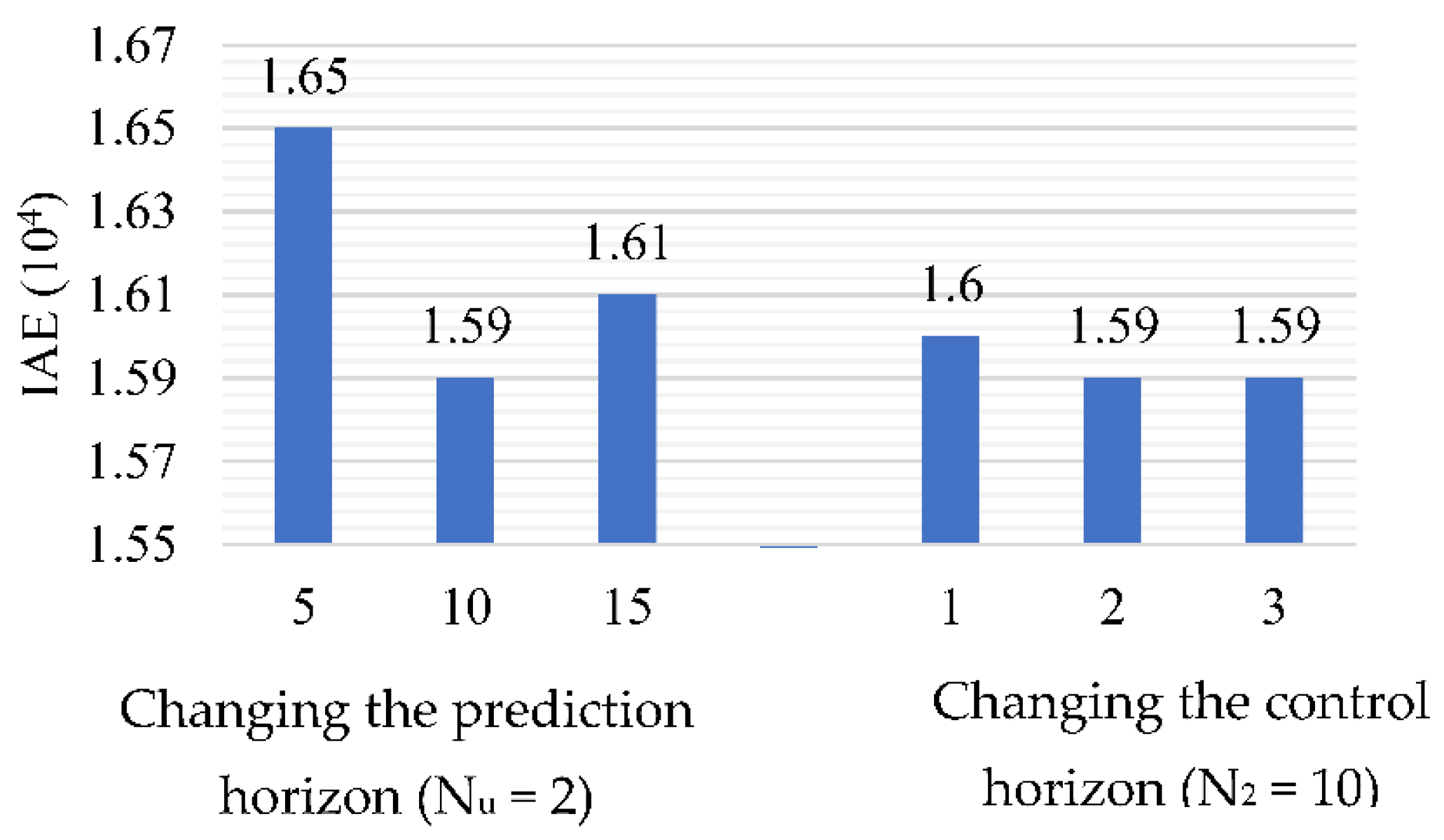
The optimal value of λ was chosen as a compromise of the two extremes, and the same procedure was carried out for different values of N₂ and N_u. The results, given in Figure 8, show that an increase in the prediction horizon from 5 to 10 significantly improved the controller performance. A further increase in N₂ caused a slight increase in IAE, likely due to a decrease in the prediction accuracy of the ARX model. Since a larger N₂ also increased the computation at each sample interval [23], a final value of N₂ = 10 was chosen.

As shown in Figure 4, the second MPC configuration used the MATLAB smoothing function to further reduce the noise in the manipulated variable. The smoothed data were then interpolated into 15 min intervals, which were used to develop a new third-order ARX model with the parameters of a₁ = −1.008, a₂ = 5.464, a₃ = 8.88, b₁ = 6.40 × 10⁻⁴, b₂ = −2.18 × 10⁻⁵, and b₃ = 2.16 × 10⁻³. The new ARX model was used in the GPC algorithm to predict measurements in the controlled variable every 15 min. Unlike conventional MPC, where only the first controller action is implemented, this method requires the first four controller actions to be implemented before the next sample is taken, and interpolation can take place again. As such, the minimum control horizon was 4.

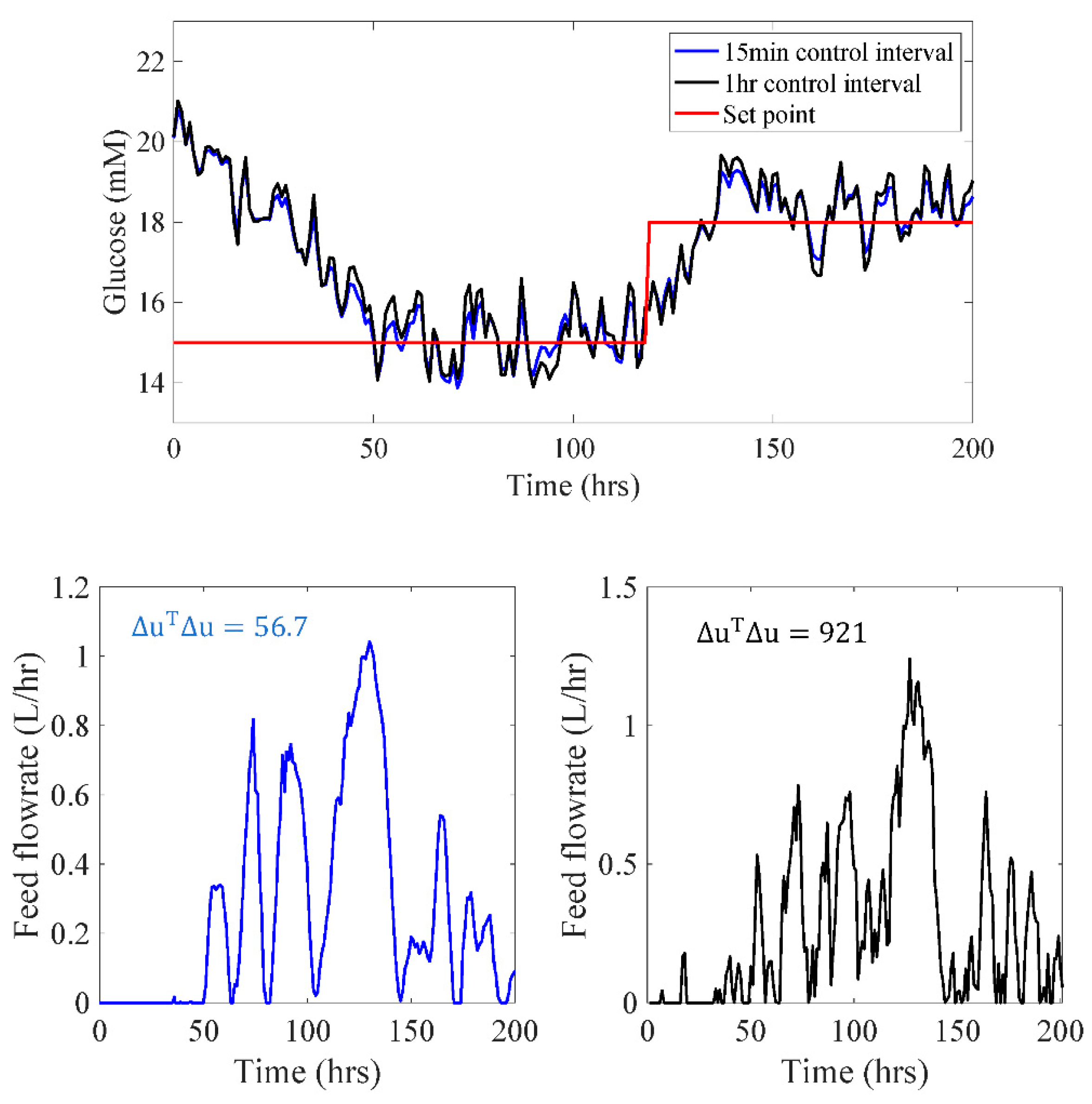
Tuning the MPC, as previously described, provided the optimal tuning parameters N₂ = 40 and N_u = 4 (given in terms of interpolated measurements rather than original samples). The results in Figure 9 show that this method is effective in removing noise from the manipulated variable, decreasing Δu^TΔu from 921 (mL min⁻¹)² to 56.7 (mL min⁻¹)². The overfeeding of glucose in the first and final 50 h was also reduced with a lower IAE (14,600 vs. 15,900). To improve the performance, a 15 min control interval was used in further comparisons.

3.1.2. Adaptive MPC

The recursive ARX model parameters were updated after each Raman sample became available to reflect the online estimates. A similar approach was previously used by Kovarova-Kovar et al. [30] to improve the data training of a data-driven model, which cannot be expected to predict data that has not been used in its training [24]. The final ARX parameters for model orders 1–3 are given in

Table 3. The ARX model parameters for model orders 1, 2, and 3 (control interval of 15 min).

Na, Nb	a1	a2	a3	b1	b2	b3
1, 1	0.998			5.55 × 10−3
2, 2	1.007	−9.1 × 10−3		5.20 × 10−4	5.05 × 10−3
3, 3	1.007	−7.16 × 10−6	−8.65 × 10−3	−4.64 × 10−2	0.100	−4.99 × 10−2

.

The disturbance being considered was a 30% increase in the theoretical cell death rate between 100 and 150 hours and the setpoint was 15 mM. In practice, a similar increase in death rate could be caused by a deviation in the fermenter temperature [31].

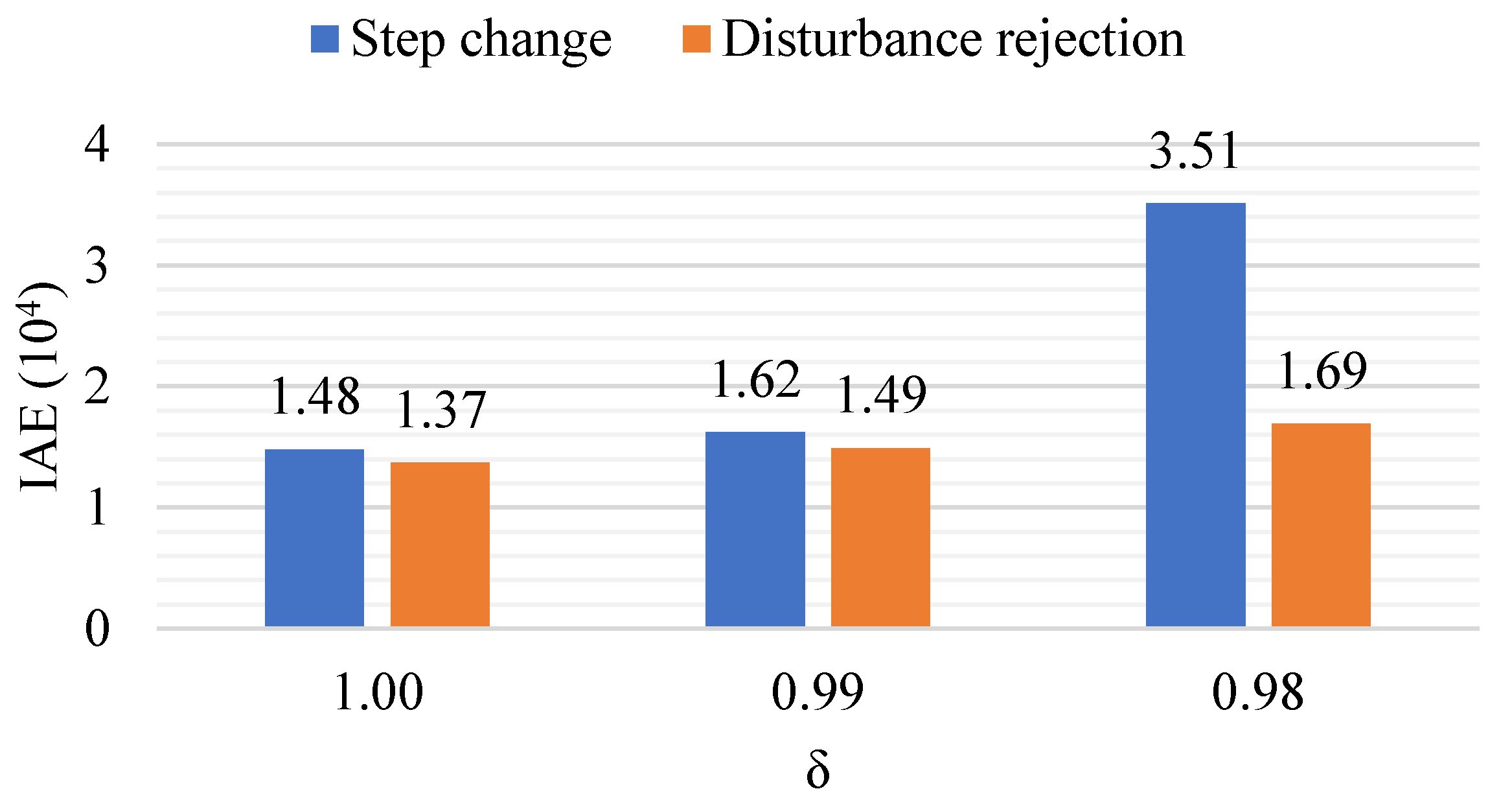
Setting the forgetting factor (δ) to 1, an initial comparison of the adaptive and non-adaptive MPC was carried out. The results showed that an adaptive controller in this configuration is ineffective, having a higher IAE for both a setpoint of 15 mM (13,500 vs. 13,600) and disturbance rejection (13,500 vs. 13,700). Decreasing δ, as shown in Figure 10, caused further deterioration in the controller performance.

Further investigation of the issue showed that the online estimation of parameters b₁ to b₃ had a wide variation, and as a result, information from the initial training was being lost.

Under a consistent feed rate, the parameters B(z⁻¹) should not be time varying. A(z⁻¹), on the other hand, represents the continuously changing reaction kinetics, for which δ < 1 would theoretically be best. As a compromise, the effect of restricting B(z⁻¹) to its initial value and having only A(z⁻¹) estimated online was considered.

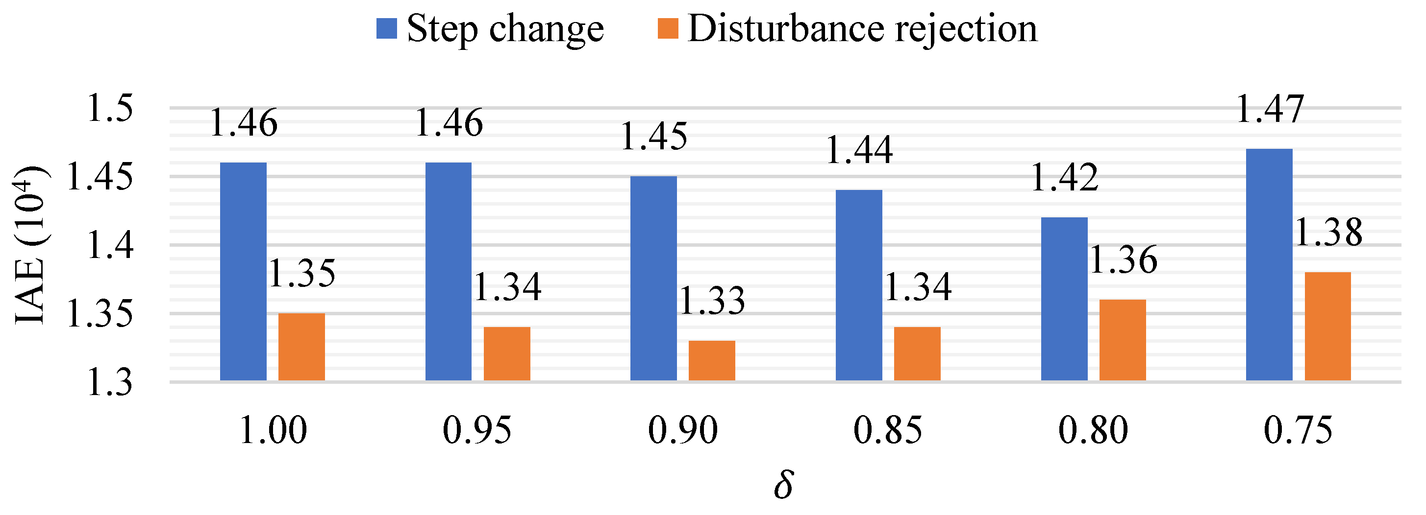
When only A(z⁻¹) was adapted online, Figure 11 shows the effect of δ on the controller response for a step change and disturbance rejection. As expected, a controller that was only adaptive in A(z⁻¹) provided a lower IAE than one that was adaptive in both A(z⁻¹) and B(z⁻¹). Decreasing δ further reduced the IAE, up to a point. A final value of δ = 0.9 was chosen for its ability to reject a disturbance with the lowest IAE.

Although the step response would suggest a smaller value be used, the objective of adaptive control is to represent the non-linearities of the reaction, as seen by a disturbance in the kinetics. The use of a step response in Figure 11 was only to confirm that data from the initial training had not been lost.

Having only A(z⁻¹) adapted online could leave the controller susceptible to disturbances in the feed composition. This was verified with a simulation using a 20% disturbance in glucose feed concentration. The results, given in

Table 4. The controller performance for a 20% increase in the glucose feed concentration between 100 and 150 h.

	IAE	ISE	ΔuTΔu
Non-adaptive	13,600	38,200	55.1
Adaptive in A and B	13,700	38,500	52.4
Adaptive in A	13,400	37,900	34.8

, show that the controller that was only adaptive in A(z⁻¹) had a lower IAE (13,400) than the one that was adaptive in both A(z⁻¹) and B(z⁻¹) (IAE = 13,700).

3.1.3. The ARX Model Order

The MPC controller design has so far assumed that a third-order model is most appropriate. This assumption can now be re-evaluated through a comparison of their adaptive and non-adaptive performance.

The results for a step change, given in

Table 5. The controller performance criteria for a step change in glucose setpoint (15 mM to 18 mM).

	Non-Adaptive MPC			Adaptive MPC
Na, Nb	IAE	ISE	$\mathsf{\Delta }{\mathit{u}}^{\mathit{T}}\mathsf{\Delta }\mathit{u}$	IAE	ISE	$\mathsf{\Delta }{\mathit{u}}^{\mathit{T}}\mathsf{\Delta }\mathit{u}$
1, 1	14,700	40,200	37.8	14,600	40,000	45.8
2, 2	14,500	40,000	40.1	14,200	39,700	43.5
3, 3	14,600	40,000	57.4	14,500	40,100	43.4

, show that using the first-order model gave the highest IAE in both the adaptive and non-adaptive configuration. The improvement seen by increasing the model order to 2, suggest that the first-order ARX model was underspecified [32].

As shown in

Table 6. The controller performance criteria for a 30% disturbance in the cell death rate.

	Non-Adaptive MPC			Adaptive MPC
Na, Nb	IAE	ISE	$\mathsf{\Delta }{\mathit{u}}^{\mathit{T}}\mathsf{\Delta }\mathit{u}$	IAE	ISE	$\mathsf{\Delta }{\mathit{u}}^{\mathit{T}}\mathsf{\Delta }\mathit{u}$
1, 1	13,500	38,100	33.5	13,600	38,100	41.2
2, 2	13,500	38,000	36.6	13,300	37,800	24.4
3, 3	13,500	38,100	54.1	13,400	37,900	34.1

, the non-adaptive second- and third-order ARX models provided a similar IAE for disturbance rejection. However, when adapted online, the second order model provided a lower IAE, ISE, and control effort. A possible cause for this is that, when adapted online, the third-order ARX model is taking on the noise of the control variable [32]. To improve its performance, a second-order ARX model will be used going forward.

3.2. PI Controller Tuning

3.2.1. PI Control without ARX Prediction

Inverse z transform of the second-order ARX model in MATLAB provided the time domain transfer function in Equation (27).

$$G_P\left(s\right)=\frac{0.0184\left(0.649s+1\right)e^{-1s}}{\left({6.81}^2\right)s^2+\left(6.81\right)\left(12.8\right)s+1}$$

(27)

Through a comparison with Equation (21), the transfer function parameters, given below, were found. These were used in Equations (22) and (23) to calculate K_c and T_i for a given value of $\lambda$.

K_m = 0.0184, T_m3 = 0.649, T_m1 = 6.81, 𝜉_𝑚 = 12.8, 𝜏_𝑚= 1.00

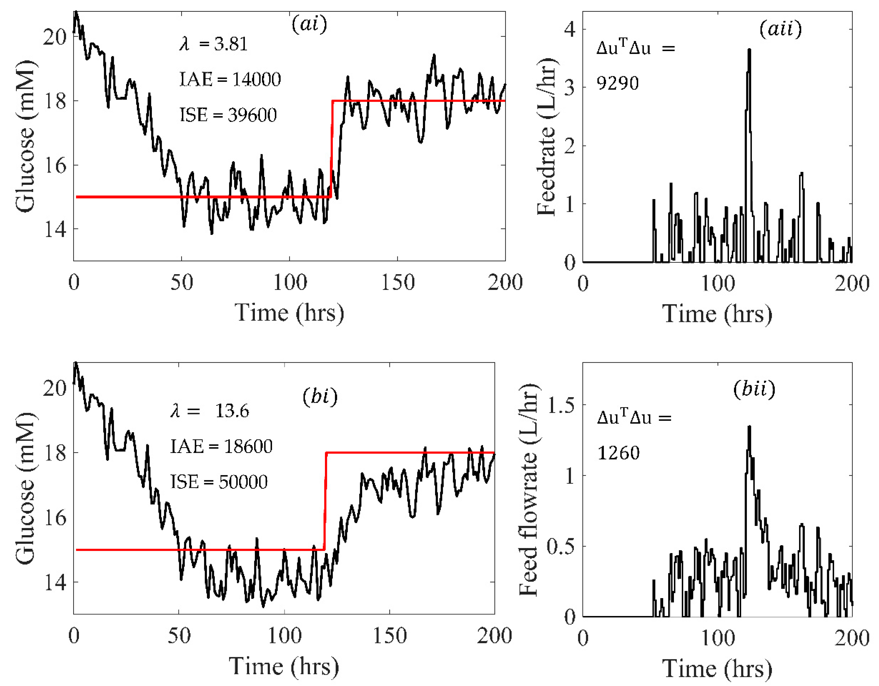
As shown in Figure 12, a small value of $\lambda$ can be used for very good controller performance to a step change in setpoint. However, this requires frequent and rapid changes in the manipulated variable. As well as causing wear on the control valve over time, such rapid changes in the manipulated variable may be unachievable in practice. Increasing $\lambda$ as shown in part b reduced Δu^TΔu, but at the expense of a sluggish response.

3.2.2. PI Control with ARX Prediction

We also considered a second PI controller configuration (see Figure 5). Here, an ARX model was used to predict future values of the control variable at 15 min intervals, allowing more frequent feedback error and changes in feed flowrate.

The PI controller was tuned using the time domain transfer function in Equation (28).

$$\mathrm{G}=\frac{0.00519\left(96.12s+1\right){\mathrm{e}}^{-15s}}{\left({17.98}^2\right)s^2+\left(17.98\right)\left(3.01\right)s+1}$$

(28)

K_m = 0.005188, T_m3 = 96.106, T_m1 = 17.983, 𝜉_𝑚 = 3.0103, 𝜏_𝑚 = 15.

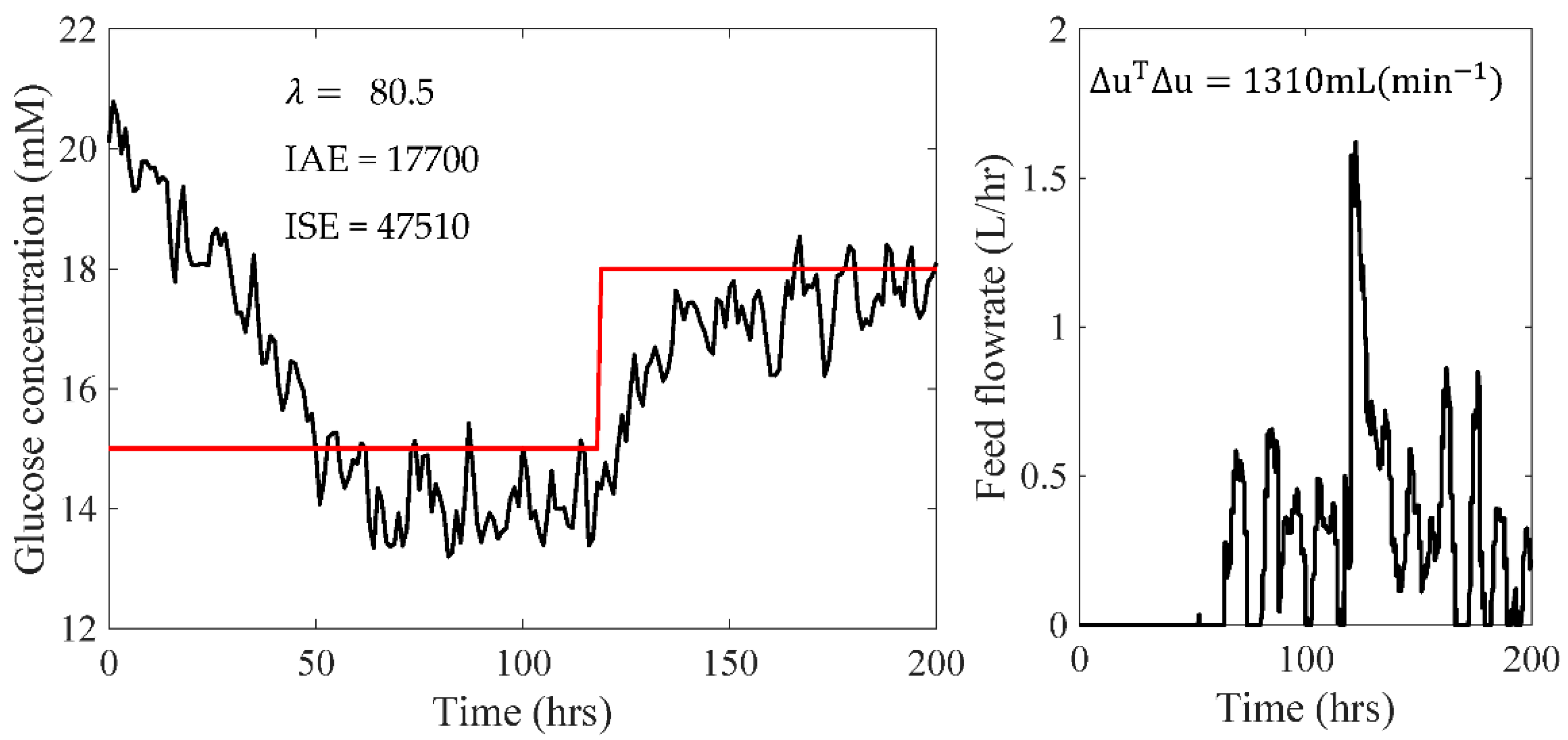
Similar to the PI control that did not use prediction, this method initially provided a low IAE (14,900), but high Δu^TΔu (5000 mL min⁻¹). Again, $\lambda$ was increased to reduce the strain on the manipulated variable. The final results, given in Figure 13, showed that for a similar change in the manipulated variable (1310 L h⁻¹ vs. 1260 L h⁻¹) the PI controller that used the ARX prediction had a lower IAE (17,700 vs. 18,600).

3.3. Robustness Analysis

3.3.1. Disturbance Rejection

The robustness of the final three controllers were evaluated by their response to disturbances in the feed composition and reaction kinetics. For the disturbance in the feed, a 20% increase in glucose concentration between 100 and 150 hours was used. In practice, a similar disturbance could be caused by poor mixing.

The results, given in

Table 7. The effect of disturbances in the feed and reaction kinetics on the IAE. (1) Setpoint 15 mM without disturbance (for reference); (2) a 20% increase in the glucose feed concentration between 100 and 150 h; (3) a 50% increase in the lag constant (Klag).

	Non-Adaptive MPC IAE	Adaptive MPC IAE	PI with Prediction IAE
1	13,500	13,300	15,900
2	13,600	13,300	15,700
3	13,600	13,400	16,000

, show that the disturbance increased the IAE of the non-adaptive MPC (13,500 vs. 13,600), but had no effect on the adaptive controller performance. The increased glucose concentration worked in favour of the PI controller, helping remove its sluggish response and therefore decreasing the IAE.

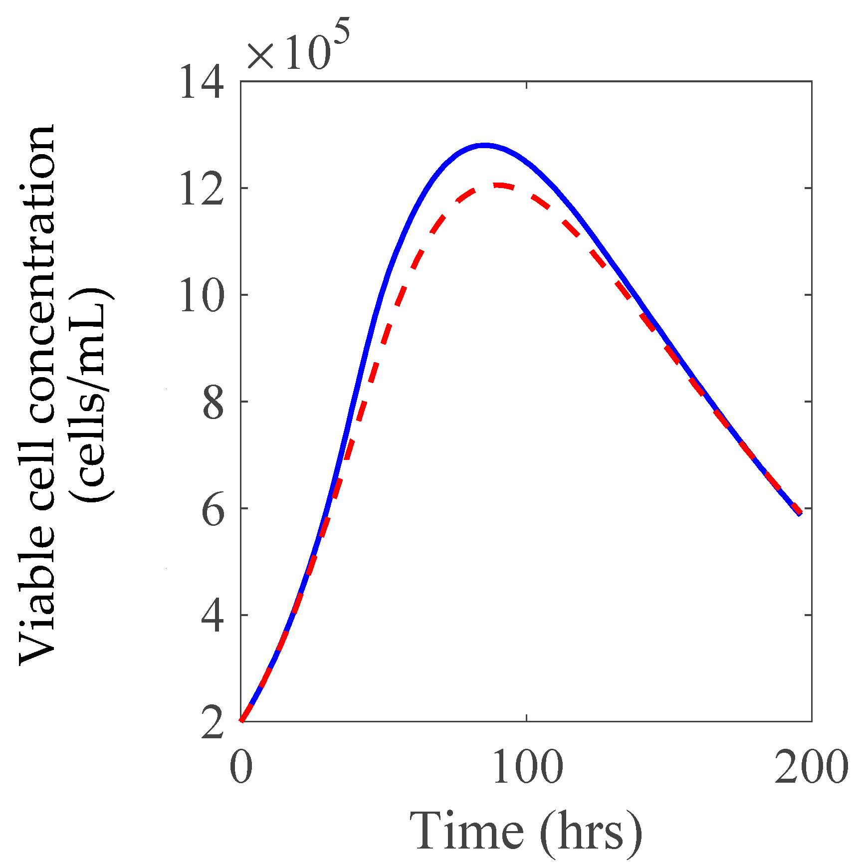
Table 7 also shows the results for a 50% increase in the lag constant (k_lag). This decreases the number of viable cells, as shown in Figure 14, and is relevant to fermentation reactions with a variable lag phase such as the one considered here [4]. The change in k_lag had a similar effect on all controllers, which saw the IAE increased by approximately 100.

Similar to the results presented by Rodrigues et al. [13], the MPC outperformed the PI control in all cases. The adaptive MPC used here consistently provided a lower IAE than its non-adaptive counterpart. This is expected for a non-linear fermentation process, which cannot be accurately represented by a linear model.

3.3.2. Changing the Sampling Time

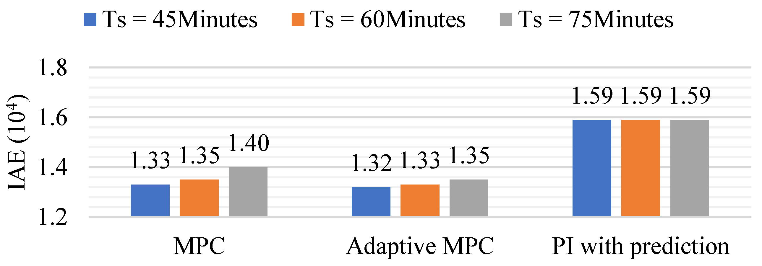
As shown in Figure 15, as the Raman sampling time increased, so did the IAE of the adaptive and non-adaptive MPC. This is similar to results presented by Rodrigues et al. [13] and is likely to have been caused by a decrease in the prediction accuracy of the ARX model at a longer sampling interval.

A change in the sampling interval was also observed to have had no effect on the PI control. The PI control works by re-calculating the controller action for each feedback error. When the change in the manipulated variable at any one time has been restricted using ω, the rapidity of changes in the manipulated variable depends only on the frequency of the feedback error. Since an ARX predictor was used for error calculations in 15 min intervals regardless of the sample time, a change in the sample interval had no effect on the PI control.

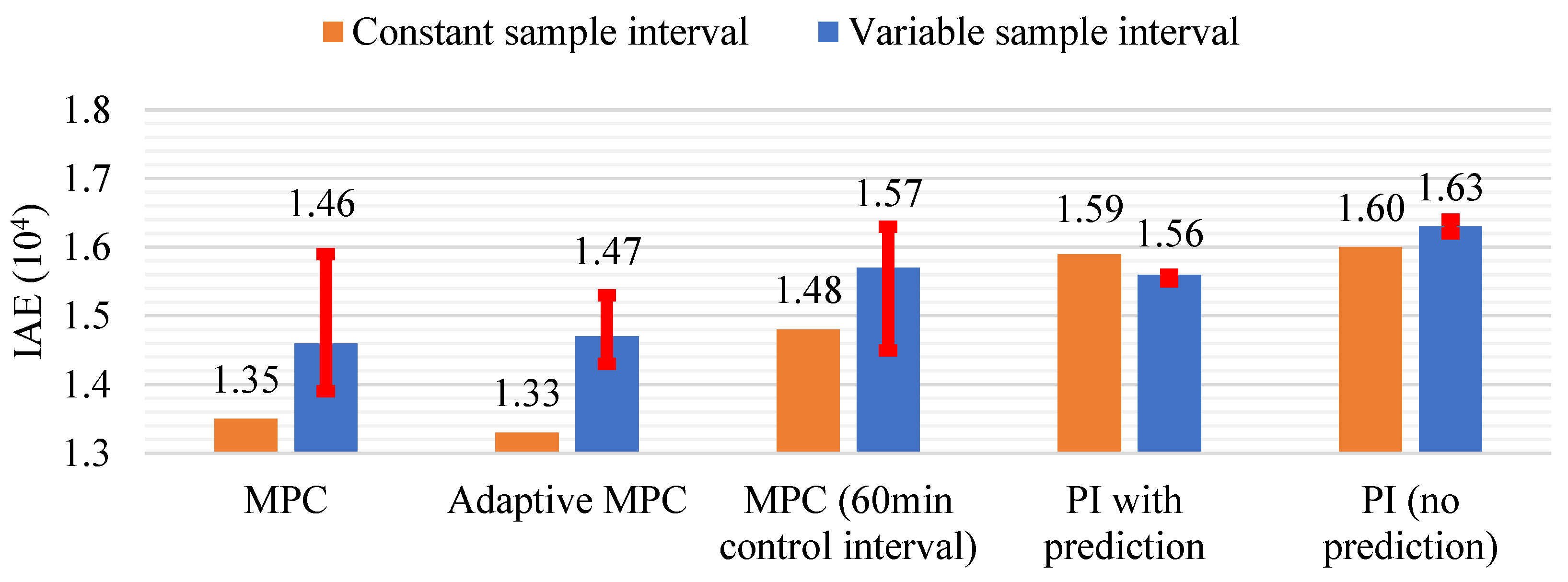
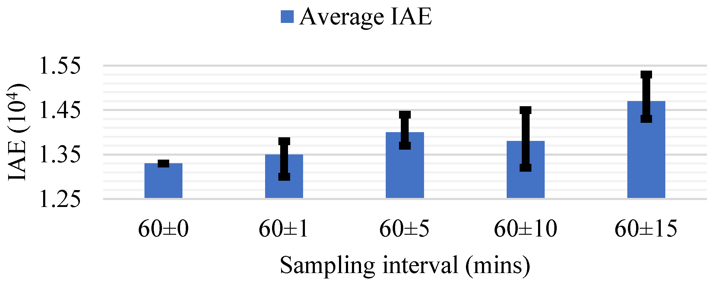
While Figure 15 would suggest the shortest possible sample interval should be used in MPC, in reality, the use of one Raman probe across multiple vessels will result in irregular sampling. To reflect this, a simulation was created in which the sampling time was varied randomly between 45 and 75 min (see Figure 6). Due to the different mode of filtering when the sample time is irregular, the comparison with a constant sample interval used the IAE, which was calculated prior to any filtering. The results through this method were taken as an average of five runs and error bars were used to show the variation in results across these runs.

The results, given in Figure 16, showed that the use of irregular sample intervals increased the average IAE for MPC. This is because the ARX model assumes that the input and output are constant between samples. When the sampling time is not restricted to a constant interval, the prediction accuracy of the ARX model decreases.

Research carried out by Khan et al. [33] was the first to address this issue by using a sampling interval that varied randomly between two values. In this, the system was modelled as a polytopic uncertain system. Unlike the ARX model, this allowed for variations in sample time as an integral part of the model. Though effective, Khan et al. [33] concluded that the high computational expense of this method may stop it from being implemented in practice, and instead, a simpler model would be required.

The results in Figure 16 show that the method proposed here, which uses an ARX model to predict the glucose concentration in 15 min intervals, reduced the error introduced by irregular sampling when compared to the MPC using a 60 min control interval. In addition, it did so without the increased computational expense of a polytopic uncertain system.

The results for PI with prediction showed that a variable sample time decreased the IAE slightly. This is because random sampling times inadvertently lead to more frequent feedback error, and therefore more frequent changes in the feed flowrate. When the feed flowrate can be changed more rapidly, the sluggish response of the PI controller improves. This idea is supported by an increase in Δu^TΔu from 673 mL min⁻¹ to 1459 mL min⁻¹ when the sampling interval was varied. Figure 17 also shows that the use of ARX prediction in PI control decreased the IAE from 16,300 to 15,600.

Despite an increase in IAE, the adaptive and non-adaptive MPC using a 15 min control interval had a lower IAE than the PI controller on average, and a significantly lower strain on the manipulated variable in all cases. The adaptive MPC had the smallest increase in average IAE when an irregular sampling interval was used, although some variation in the results remained. When used in practice, this variation should be minimised by restricting the variation in the sampling time (see Figure 17).

As well as variations in sampling time, process model mismatch (PPM) between the model used in MPC development and a real process is a potential source of controller error. Although the model was validated with laboratory experiments by Kiparissides et al. [19], the assumption that the reaction kinetics remain constant when scaled up may not be true in practice. The implementation of the MPC on an industrial fermentation process would be required to see if this is the case. If the controller performance deteriorates in this situation, the MPC should be re-tuned, as seen in the study by Craven et al. [5].

4. Conclusions

This study shows how a linear ARX model can be used to predict more frequent measurements of the controlled variable and improve the controller performance when Raman measurements are taken infrequently. The proposed method was applied to glucose concentration control in a simulation of mAb production, with hourly measurements interpolated into 15 min intervals and smoothed to reduce noise. When used in the GPC algorithm, these more frequent measurements reduced the IAE from 15,900 to 14,600. As expected, the online adaptation of the linear ARX model further reduced the IAE for setpoint tracking (14,200 vs. 14,500) and disturbance in the reaction kinetics (13,300 vs. 13,500).

The same method of ARX prediction improved the conventional PI control, reducing the IAE from 18,600 to 17,700 for a step change in glucose concentration. Despite this, both adaptive and non-adaptive MPC outperformed the PI controller, having a lower IAE, ISE, and control effort (Δu^TΔu) for setpoint tracking.

A final comparison showed the effect of irregular sampling on the control performance with and without ARX prediction. For both MPC and the PI control, the use of an ARX predictor improved controller performance. Adaptive MPC had the lowest IAE on average, though the results varied run-to-run. If adaptive MPC is to be implemented in practice, this variation should be minimised by restricting the variation in the sample interval as much as possible. In future works, non-linear adaptive dynamic models implemented through neural networks such as extreme learning machine will be investigated to cope with the non-linearities commonly existing in batch processes. Extreme learning machine is shown to have fast training and is suitable for online model adaptation.

References

- Budzinski, K.L.; Koenig, S.G.; O’Connor, D.A.; Wu, T.S. A call for industry to embrace green biopharma. Nat. Biotechnol. 2016, 34, 234–235. [Google Scholar] [CrossRef] [PubMed]
- Maruthamuthu, M.K.; Rudge, S.R.; Ardekani, A.M.; Ladisch, M.R.; Verma, M.S. Process analytical technologies and data analytics for the manufacture of monoclonal antibodies. Trends Biotechnol. 2020, 38, 1169–1186. [Google Scholar] [CrossRef] [PubMed]
- World Health Organization. Medicines: Good Manufacturing Practices. 2015. Available online: https://www.who.int/news-room/q-a-detail/medicines-good-manufacturing-processes (accessed on 26 June 2022).
- Vermeersch, L.; Perez-Samper, G.; Cerulus, B.; Jariani, A.; Gallone, B.; Voordeckers, K.; Steensels, J.; Verstrepen, K.J. On the duration of the microbial lag phase. Curr. Genet. 2019, 65, 721–727. [Google Scholar] [CrossRef] [Green Version]
- Craven, S.; Whelan, J.; Glennon, B. Glucose concentration control of a fed-batch mammalian cell bioprocess using a nonlinear model predictive controller. J. Process Control 2014, 24, 344–357. [Google Scholar] [CrossRef]
- Wallocha, T.; Popp, O. Off-Gas-Based Soft Sensor for Real-Time Monitoring of Biomass and Metabolism in Chinese Hamster Ovary Cell Continuous Processes in Single-Use Bioreactors. Processes 2021, 9, 2073. [Google Scholar] [CrossRef]
- Nguyen, N.B.T.; Lin, G.-H.; Dang, T.-T. Fuzzy multi-criteria decision-making approach for online food delivery (OFD) companies evaluation and selection: A case study in Vietnam. Processes 2021, 9, 1274. [Google Scholar] [CrossRef]
- FDA. Guidance for Industry PAT—A Framework for Innovative Pharmaceutical Development, Manufacture and Quality Assurance. 2004. Available online: https://www.fda.gov/regulatory-information/search-fda-guidance-documents/pat-framework-innovative-pharmaceutical-development-manufacturing-and-quality-assurance (accessed on 26 June 2022).
- Becker, T.; Hitzmann, B.; Muffler, K.; Portner, R.; Reardonm, K.F.; Stahl, F.; Roland, U. Future aspects of bioprocess monitoring. In Advances in Biochemical Engineering/Biotechnology; Scheper, T., Ulber, R., Sell, D., Eds.; Springer: Berlin, Germany, 2007; pp. 251–255. [Google Scholar]
- Abu-Absi, N.R.; Kenty, B.M.; MCuellar, M.E.; Borys, M.C.; Sakhamuri, S.; Strachan, D.J.; Hausladen, M.C.; Li, Z.J. Real time monitoring of multiple parameters in mammalian cell culture bioreactors using an in-line Raman spectroscopy probe. Biotechnol. Bioeng. 2011, 108, 1215–1221. [Google Scholar] [CrossRef]
- Whelan, J.; Craven, S.; Glennon, B. In situ Raman spectroscopy for simultaneous monitoring of multiple process parameters in mammalian cell culture bioreactors. Biotechnol. Prog. 2012, 28, 1355–1362. [Google Scholar] [CrossRef]
- Mohd, N.; Aziz, N. Performance and robustness evaluation of nonlinear autoregressive with exogenous input model predictive control in controlling industrial fermentation process. J. Clean. Prod. 2016, 136, 42–50. [Google Scholar] [CrossRef]
- Rodrigues, J.A.; Toledo, E.C.; Filho, R.M. A tuned approach of the predictive–adaptive GPC controller applied to a fed-batch bioreactor using complete factorial design. Comput. Chem. Eng. 2002, 26, 1493–1500. [Google Scholar] [CrossRef]
- Wang, Z.; Georgakis, C. Identification of Hammerstein-Weiner models for nonlinear MPC from infrequent measurements in batch processes. J. Process Control 2019, 82, 58–69. [Google Scholar] [CrossRef]
- Gopalakrishnan, A.; Kaisare, N.S.; Narasimhan, S. Incorporating delayed and infrequent measurements in Extended Kalman Filter based nonlinear state estimation. J. Process Control 2011, 21, 119–129. [Google Scholar] [CrossRef]
- Li, D.; Shah, S.L.; Chen, T.; Qi, K.Z. Application of dual-rate modeling to CCR octane quality inferential control. IEEE Trans. Control Syst. Technol. 2003, 11, 43–51. [Google Scholar] [CrossRef] [Green Version]
- Mosalanejad, M.; Arefi, M.M. UKF-based soft sensor design for joint estimation of chemical processes with multisensor information fusion and infrequent measurements. IET Sci. Meas. Technol. 2018, 12, 755–763. [Google Scholar] [CrossRef]
- Box, G.P.; Hunter, W.G.; Hunter, J.S. Statistics for Experiments: An Introduction to Design, Data Analysis, and Model Building; John Wiley & Sons: Hoboken, NJ, USA, 1978. [Google Scholar]
- Kiparissides, A.; Pistokopoulos, E.N.; Mantalaris, A. On the model-based optimization of secreting mammalian cell (GS_NS0) cultures. Biotechnol. Bioeng. 2014, 112, 536–548. [Google Scholar] [CrossRef]
- Yang, J.D.; Lu, C.; Stasny, B.; Henley, J.; Guinto, W.; Gonzalez, C.; Gleason, J.; Fung, M.; Collopy, B.; Benjamino, M.; et al. Fed-batch bioreactor process scale-up from 3L to 2,500L scale for monoclonal antibody production from cell culture. Biotechnol. Bioeng. 2007, 98, 141–154. [Google Scholar] [CrossRef]
- Hu, W.S. Cell Culture Bioprocess Engineering; CRC Press: Boca Raton, FL, USA, 2020. [Google Scholar]
- Mahdinia, E.; Cekmecelioglu, D.; Demirci, A. Bioreactor scale-up. In Essentials in Fermentation Technology; Berenjian, A., Ed.; Springer: Berlin/Heidelberg, Germany, 2019; pp. 213–236. [Google Scholar]
- Clarke, D.W.; Mohtadi, C.; Tuffs, P.S. Generalised predictive control—Part I: The basic algorithm. Automatica 1987, 23, 137–148. [Google Scholar] [CrossRef]
- Qin, S.J.; Badgwell, T.A. A survey of industrial model predictive control technology. Control Eng. Pract. 2003, 11, 733–764. [Google Scholar] [CrossRef]
- Zhang, H.; Lennox, B. Integrated condition monitoring and control of fed-batch fermentation processes. J. Process Control. 2004, 14, 41–50. [Google Scholar] [CrossRef]
- Camacho, E.F.; Bordons, C. Model Predictive Control; Springer: London, UK, 2007. [Google Scholar]
- King, M. Process Control—A Practical Approach, 2nd ed.; John Wiley & Sons: Hoboken, NJ, USA, 2016. [Google Scholar]
- Rohani, S. Coulson and Richardson’s Chemical Engineering, Volume 3B—Process Control, 4th ed.; Elsevier: Amsterdam, The Netherlands, 2017. [Google Scholar]
- O’Dwyer, A. Handbook of PI and PID Controller Tuning Rules, 3rd ed.; World Scientific: Singapore, 2009. [Google Scholar]
- Kovarova-Kovar, K.; Gehlen, S.; Kunze, A.; Keller, T.; Daniken, R.V.; Kolb, M.; van Loon, A.P. Application of model-predictive control based on artificial neural networks to optimize the fed-batch process for riboflabin production. J. Biotechnol. 2000, 79, 39–52. [Google Scholar] [CrossRef]
- Atala, D.I.; Costa, A.C.; Maciel, R.; Maugeri, F. Kinetics of ethanol fermentation with high biomass concentration considering the effects of temperature. Appl. Biochem. Biotechnol. 2001, 91, 353–365. [Google Scholar] [CrossRef]
- Zhu, Y. Extensions of the least-squares method. In Multivariable System Identification for Process Control; Pergamon: Oxford, UK, 2001; pp. 97–157. [Google Scholar]
- Khan, O.; Mustafa, G.; Khan, A.Q.; Abid, M. Robust observer-based model predictive control of non-uniformly sampled systems. ISA Trans. 2020, 98, 37–46. [Google Scholar] [CrossRef] [PubMed]
Figure 1.
The true glucose concentration and infrequent measurement with noise when Fin = 0 L h−1.
Figure 2.
The glucose concentration and feed flowrate in the ARX data training.
Figure 3.
The adaptive MPC.
Figure 4.
Illustration of the MPC.
Figure 5.
The two feedback control configurations: (a) standard feedback control, (b) with prediction of more frequent values.
Figure 6.
The sample time variations between 45 and 75 min.
Figure 7.
The control performance for a step change in setpoint (N2 = 10, Nu = 2): (ai), λ = 5 × 10⁻⁴, controlled variable (blue) and setpoint (red); (aii), λ = 5 × 10⁻⁴, manipulated variable; (bi), λ = 5 × 10⁻⁴, controlled variable (blue) and setpoint (red); (bii), λ = 5 × 10⁻⁴, manipulated variable.
Figure 8.
The effect of the prediction and control horizons on IAE.
Figure 9.
A comparison of the MPC performance for control intervals of 1 h and 15 min.
Figure 10.
The effect of the forgetting factor () on the adaptive controller performance.
Figure 11.
The effect of on the MPC performance that was adaptive only in A(z−1).
Figure 12.
The effect of λ on the PI controller performance: (ai), λ = 3.81, controlled variable (black) and setpoint (red); (aii), λ = 3.81, manipulated variable; (bi), λ = 13.6, controlled variable (black) and setpoint (red); (bii), λ =13.6, manipulated variable.
Figure 13.
The setpoint tracking performance of a PI controller with ARX prediction: (left): controlled variable (black) and setpoint (red); (right): manipulated variable.
Figure 14.
The effect of a 50% increase in Klag on the viable cell concentration, blue: no disturbance, red: with disturbance.
Figure 15.
The effect of sampling time on the controller performance.
Figure 16.
The effect of a variable sampling time (60 ± 15 min) on the controller performance. Results taken as an average of five runs and error bars (red) included to show the variation in IAE.
Figure 17.
The effect of increased variation in the sampling time on the controller performance. The results taken as an average of five runs and error bars (black) were included to show the variation in the IAE in these runs.