
A Development of an Induction Heating Process for a Jewelry Factory: Experiments and Multiphysics


Computer Simulation in Engineering Research Group, College of Advanced Manufacturing Innovation, King Mongkut’s Institute of Technology Ladkrabang, Bangkok 10520, Thailand
*
Author to whom correspondence should be addressed.
Processes 2023, 11(3), 858; https://0-doi-org.brum.beds.ac.uk/10.3390/pr11030858
Submission received: 17 January 2023
/
Revised: 27 February 2023
/
Accepted: 8 March 2023
/
Published: 13 March 2023
(This article belongs to the Special Issue Green Manufacturing and Sustainable Supply Chain Management)
Abstract
:This article reports a successful development of the induction heating process (IHP) in a jewelry factory based on experiments and multiphysics consisting of electromagnetic and thermal simulations. First, two experiments were set to measure essential parameters for result validation and multiphysics boundary condition settings. Then, the essential parameters were applied to multiphysics, and both simulation results revealed heat transfer, magnetic flux density (B) generated by the coil, and temperature (T) of the product. B and T were consistent with the experimental results and theory, confirming the reliability of the multiphysics and methodology. After that, all simulation results were analyzed to assess and optimize IHP in terms of the number of coil turns (N), positional placement of the product (P), and coil thickness (Th). Multiphysics revealed that the current operating condition with N = 3 is proper; however, the IHP can be improved more with coil and operating condition optimizations. Finally, completing the optimizations, decreasing 40% of Th with N = 6, and the same P, increased B on the product by 21.62%, leading to IHP efficacy enhancement. The research findings are the optimum coil model and methodology for developing the IHP, which were practically employed in the jewelry factory.
1. Introduction
Thailand is the world’s major gem and jewelry manufacturing base. In 2016, Thailand was the number one exporter in Asia, with an export value of more than 14.2 billion dollars. The main export products were gold (rank 20), silver jewelry (rank 2), gold jewelry (rank 13), and gemstone cutting (rank 2) [1]. The numbers in parentheses are the world rankings for each category reported in 2016. In 2021, the export value was approximately 6.2 billion dollars, down from 2016 because of COVID-19. However, it is growing more every month in 2022 than last year as the disease eases and the Thai baht decreases; therefore, Thai manufacturers have a bright export prospect [1]. With a large production volume, as mentioned above, Thai manufacturers must have modern and effective technology that is cost-efficient, fast in manufacturing, and creates high-quality products. Accordingly, the induction heating process (IHP) is one of the technologies that Thai manufacturers have successfully developed on their own.
The IHP in a jewelry factory is the process of joining different types of precious metals together to form a product by melting solder under the heat generated by induction, called induction heating. Figure 1 shows gold and silver necklaces as product examples from a jewelry factory. Dash boxes present components produced by the IHP. In detail, industrial applications of induction heating can be divided into five groups: heat treating, mass heating, melting, welding, and special applications [2]. All relate to metallurgical processes. For example, in heat treatment, induction is used in processes such as hardening, tempering, annealing, sintering, etc., to change the metallurgical properties. Mass heating is employed in wire and cable heating to dry post-cleaning or remove water and solvent from the coating. Additionally, it is used in slug heating for semisolid forming, etc. Melting applies induction to raise the temperature of metal or ore to its melting point and hold that temperature to perform metallurgical processes such as smelting, alloying, mixing, casting, etc. Welding mainly uses induction to connect the same type of products joined together. Lastly, special applications use brazing, bonding, soldering, etc., to join different types of products together by melting solder. The IHP in a jewelry factory is one of the benefits of the last application, special applications. With so many benefits, IHP has been studied and developed rapidly for many purposes nowadays [2,3].
Before the 2010s, engineers at the factory preferred to use a trial-and-error method to investigate and develop the IHP. However, unfortunately, this method consumes budget and time. In addition, electromagnetic fields, currents, temperatures, etc., and physical phenomena related to IHP are challenging to investigate with the naked eye. These are the main obstacles to developing IHP. Nowadays, computers and software are becoming more powerful, so developers and researchers prefer to apply multiphysics, a simulation method that relies on a computer’s and software’s high capabilities, to develop the IHP [4,5,6,7,8,9]. For example, Kranjc et al. [4], Chen et al. [5], and Luozzo et al. [6] initiated multiphysics to study induction heating. Unfortunately, their sample products were a solid cylinder [4], a thin bar [5], and tubes [6], the simplest shapes, studied by applying simple operating conditions; therefore, their simulation results were accurate but had a limit on practical application. However, all contribute to understanding induction heating, leading to other research later. Subsequently, multiphysics was applied to products with more complex shapes, such as Jianliang et al. [7] for heavy cylinders, Choi et al. [8] for AISI1045 cylinders, and Ahn et al. [9] for cylindrical concretes, under realistic operating conditions. All confirmed that operating conditions suitable for the product properties would provide the most efficient IHP; therefore, both are vital factors to be considered and designed before actual uses. However, all that is mentioned above is basic and cannot be applied to actual jewelry manufacturing.
This article reports on the successful use of experiments and multiphysics for developing IHP in a Thai manufacturer’s jewelry factory, which is more advanced than the research mentioned above [4,5,6,7,8,9], aimed to resolve a product defect problem, improve the manufacturing process to be more efficient, and understand IHP. First, an operating condition and a specification of the induction heating machine implemented in the actual IHP were collected. Next, experiments to mimic the actual IHP were set in a laboratory. Then, the IHP was tested by using the same operating conditions as in the factory to gather parameters for setting in multiphysics and validation. Afterward, the multiphysics consisting of electromagnetic and thermal simulations was employed to investigate the magnetic field, heat transfer, and an implication with the defect. Finally, all experimental and simulation results were analyzed and optimized, developing IHP to achieve all mentioned aims.
Since the outcomes of this research must be applied to the factory and the products are tiny, assembled with many types of materials, the research methodology is more complicated and realistic. Accordingly, the focus of this research is the experimental and multiphysics settings designed exclusively to get reliable and practical results.
2. Theoretical Background
This section is a brief on the principles of induction, IHP mechanisms, and multiphysics, which consist of governing finite element equations for electromagnetic and thermal simulations.
2.1. Principles of Induction Heating
Induction heating is a process for heating metals or electrically conductive materials. It is commonly used in jewelry factories because of its precision, cost-effectiveness, repeatability, and safety with a noncontact method. However, it must be carefully controlled since it involves a high current that generates a harsh temperature. The principles of induction heating include Maxwell’s equation, Joule’s heating, the skin effect, and heat transfer, which are described below.
2.1.1. Maxwell’s Equation
Figure 2 shows the equipment for induction heating, including currents and magnetic fields, viewed from (a) the side and (b) the top to link with the IHP. The important equipment consists of a product to be heated and a coil. In (a), when an alternating current (yellow) is applied to the coil, it results in a time-varying applied magnetic field (green) with a direction obeying a right-hand rule. After that, if the product is placed stationary in the applied magnetic field, it causes an induced current (also called eddy current, red) and an induced magnetic field (blue) inside the product in the direction opposing the applied current and magnetic field due to Lenz’s law. In (b), the directions of the mentioned magnetic fields and currents are revealed in detail. Accordingly, this eddy current produces heat by the Joule’s effect (also known as the Joule’s heating), and the product is heated.
In detail, the currents and magnetic fields described above can be determined by solving Maxwell’s equations given in [6].
where is the volume electric charge density, is the electric current density, is the permittivity, is the permeability, is the electric field, and is the magnetic field. The Equations (1)–(4) are recognized as Gauss’s law for electricity, Gauss’s law for magnetism, Faraday’s law, and Ampere’s law, respectively. The bold means a vector.
From Equation (4), it can be proved that for a circular wire with a radius R, the B at a center position is:
where N is the number of coil turns, B is the magnetic flux density, and μ0 is the permeability of free space. This equation, called the Biot–Savart’s law, is used to help with analysis and discussion.
2.1.2. Joule’s Heating
The governing equation of Joule’s heating can be expressed by:
where is the power, is the eddy current, and is the coil’s resistance.
In a simple summary of Equations (1)–(6), the greater the applied current, the greater the eddy current, resulting in a great temperature inside the product. Moreover, a coil design, product shape, and material properties affect heat induction.
2.1.3. Skin Effect
Since the product is an electrically conductive material, the eddy current tends to concentrate on the outer surface rather than the inner surface. Accordingly, the heat prefers dissipating on the outer surface at a distance not greater than δ from the surface, called the skin depth. It can be calculated by [10]:
where is the electrical resistivity, is the frequency of the alternating current, and is the magnetic permeability.
From Equation (7), the higher the frequency, the smaller the skin depth. In multiphysics, the skin depth helps to define boundary conditions. The skin depth involving boundary conditions will be discussed again in Section 3.3, multiphysics.
2.1.4. Heat Transfer
As mentioned above, the skin effect makes the eddy current distributed near the product’s outer surface; also, heat would be high in that region. Thus, the outer region acts as a heat source to transfer heat to the inner region, that is, occurring heat transfer.
Accordingly, inside the product, the temperature of an isotropic material can be calculated by solving [6]:
where is the mass density, is the material conductivity, is the specific heat capacity, is the temperature, is the volumetric power density or internal heat source, and is the time.
In addition, the radiation and convection of the product surface are governed by:
where is the convection coefficient, is the normal unit vector, is the material emissivity, and is the Stefan–Boltzman constant. The subscription amb is for the ambient value.
2.2. IHP Mechanism
The material types and rough dimensions to manufacture necklaces in the marked area of Figure 1 can be modified and presented in a 2D cross-section, material types, and rough dimensions, as seen in Figure 3. In this research, the silver necklace is a case study because of its mass production in Thailand. The materials consist of a chain (blue), solder (yellow), end capsule (grey), and jig (green). The chain and end capsule are composed of 90% silver and 10% copper, while the solder is 70% silver and 30% copper. Please note that the percentage of materials and shape design depend on the manufacturer. Some manufacturers may mix it with other metals and change the percentages for durability and specific purposes. The end capsule is hollow with a hook on the bottom. The jig is composed of ceramic to hold the materials mentioned above stationary. It has an open hole allowing air (white) to help the temperature distribute entirely all over the end capsule’s surface.
First, the IHP mechanism begins with an operator of a jewelry factory inserting the end capsule into the jig and then moving the jig to the induction heating machine. Then, a solder was placed into the hollow of the end capsule. Next, the chain was pressed down onto the solder, switched on to the induction heating machine, and waited for approximately 7 s. Finally, the operator removed the product from the induction heating machine and removed the jig. Accordingly, the solder melted at approximately 779 °C based on the physics principle of induction heating described in Section 2.1, filling and spreading all over the hollow to connect the chain and end capsule together.
If the IHP was complete, all materials would be perfectly aligned, as shown in Figure 3. However, if the IHP was incomplete, the solder did not melt completely; therefore, the defect occurred. For this product, the temperature should not exceed 870 °C to prevent the end capsule and chain from melting, including not below 779 °C in the hollow region to melt the solder. Noticeably, the defect was caused by unsuitable heat transfer from the induction heating machine, higher or lower than the mentioned temperature. Excessive heat on the product leads to a burn defect resulting from silver to charcoal degradation on the product surface. On the contrary, insufficient heat on the product causes an unbinding defect from the solder unmelting; therefore, the chain and end capsule are disconnected. Thereby, investigating and developing the IHP based on multiphysics can solve the defects. In addition, comparing the products in [4,5,6,7,8,9], our product is so tiny with more material types; thus, it makes this research more challenging.
Why is this research more challenging? It is because we are employing multiphysics. The relevance of the skin depth, the end capsule’s thickness, and the material types employed in this case study to generate the induction heating affect multiphysics settings. From the authors’ experience, the end capsule’s thickness for this product is 1.0 mm, marked as red text in Figure 3; therefore, using Equation (7), the skin depth should not exceed 1.0 mm either. In this case, it was 0.26 mm. If the skin depth is less than 1.0 mm, multiphysics is a one-way simulation with coupling between electromagnetic and thermal simulations. On the other hand, if the skin depth is deeper than 1.0 mm, higher than the end capsule’s thickness, the electromagnetic wave penetrates longer into the solder, hole, or chain. This leads to only electromagnetic simulation, requiring complicated experiments to support boundary condition settings, more computation resources, and more time.
2.3. Multiphysics
Or multiphysics simulation is generally referred to as the process of computer simulation of a couple or more physical phenomena. In industrial factories, multiphysics is very useful in improving and developing the manufacturing process [11,12,13,14,15,16,17,18]. For example, in multiphysics usage, Thongsri et al. [11,12] employed thermal, electric, and structural simulations to investigate heat transfer for improving the reflow soldering process in a hard disk drive factory. Likewise, computational fluid dynamics and harmonic response analysis were applied by Tangsopa et al. [13,14] to design industrial factories’ proper ultrasonic cleaning tanks. Furthermore, structural and acoustic simulations were applied by Srathonghuam et al. [15] to develop a submersible ultrasonic transducer for an application in the inhibitory activity of pathogenic bacteria for a transducer factory. Again, Phophayu et al. [16] employed both simulations to develop industrial ultrasonic cleaning tanks and investigate the material building tank effect on cleaning efficacy. Recently, fluid flow, heat transfer, and structural simulations were applied by Thongsri et al. [17] to solve a housing damage problem in a gas turbine power plant and an excessive ablation problem inside a supersonic rocket nozzle [18] for a weapon factory.
However, multiphysics for induction heating entirely differs from the work mentioned above [11,12,13,14,15,16,17,18]. As described in Section 2.1, it consists of electromagnetic and thermal simulations; therefore, this research employs Ansys Maxwell 2022 R1 and thermal simulations. Ansys Maxwell is one of the famous commercial software for electromagnetic simulation [19,20,21,22]. For example, Tikhonova et al. [19,20] used it to design induction motors to achieve high efficiency. Furthermore, Özüpak [21] applied it to find an optimal design for a transformer. Pawar et al. [22] recently used Ansys Maxwell to develop an electromagnetic forming process. Ansys Maxwell is a widely applied transformer, coil, and motor design. However, it is still very rarely used in the study of induction heating, especially when a process has the complexity depicted in Figure 3. Evidently, using Ansys Maxwell challenges us; therefore, a brief description of Ansys Maxwell and its governing equations is provided below.
Ansys Maxwell 2022 R1 is a computer simulation software based on the finite element method (FEM). The FEM converts electromagnetic, Maxwell’s Equations (1)–(4) to [23].
where , , and are the stiffness, magnetic field, and electric current density matrices, respectively.
The crucial benefit of this software includes its adaptive mesh capability. In fact, the mesh model for electromagnetic simulation, a process to create elements and nodes in the FEM, relates to frequency. Accordingly, the mesh needs at least six elements per wavelength to predict an accurate physical phenomenon [13,14,15,16]. This consumes enormous computational resources and time, but Ansys Maxwell automatically provides the adaptive mesh capability as a default setting, facilitating users.
The adaptive mesh is a capability that automatically changes the elements’ size and node numbers to match the complexity of the physical phenomena. However, without the adaptive mesh capability, users must write computational codes by themselves, significantly depending on topics, as seen in [24], or using a mesh-independent analysis method, as employed in [11,12,13,14,15,16,17,18]. For the convenience of users is why we use this software. In addition, since Equation (10) represents all four of Maxwell’s Equations (1)–(4), it needs more computational resources to succeed. Thus, a multiphysics setting by calculating Equation (10) with the least computational resources is the way to succeed in this research, which is a one-way simulation, a coupling between electromagnetic and thermal simulations. After completing Equation (10), the Ansys Maxwell can present many results, such as electric field, magnetic field, ohmic loss, etc. Unfortunately, this software cannot present thermal results; therefore, a one-way simulation, coupling the Ansys Maxwell and thermal simulations, was employed.
As described in Section 2.2, the calculated results from Equation (10) are applied as loads to Ansys’s thermal simulation for the one-way simulation. This simulation transforms heat transfer Equations (8) and (9) to [17,18]:
where is the thermal capacitance matrix, is the thermal stiffness matrix, is the external-thermal vector load, is the change in nodal vector temperature, and is the nodal vector temperature.
In summary, multiphysics numerically solves Equations (10) and (11) to find the product temperature and magnetic fields in materials and space.
3. Methodology
This section is divided into IHP (red), experiments (yellow), and multiphysics (green), presented as a flowchart of methodology in Figure 4. All are briefly summarized and reported below.
3.1. IHP in a Jewelry Factory
This section describes the induction heating machine and the essential parameters for a simulation’s success. All were collected from the jewelry factory as information to design experiments and simulations with multiphysics.
3.1.1. Induction Heating Machine
It consists of an induction heating generator, transformer, and coil, as shown in a diagram in Figure 5. Inside the generator are a rectifier, filter, and resonant inverter. When an alternating current (AC) is applied to the generator, the current will pass through a rectifier circuit to convert AC to direct current (DC). Then, the DC passes through a filter to enhance the DC quality and smoothness. Next, it passes to a resonant inverter, which adapts the DC to AC again. Depending on operating conditions, users can adjust the output current (I1) released from the resonant inverter. Significantly, adjusting I1 will cause the frequency to change as well. After that, I1 passes to a step-down transformer with a turn ratio (TR) of 16, increasing the current to I2 with the same frequency. Finally, I2, the applied current, is driven to a coil, leading to induction heating.
3.1.2. Essential Parameters
In actual manufacturing, all materials were prepared to be a product. Each product (necklace in this case) requires different operating conditions. The induction heating machine can control a product’s temperature by adjusting I2 and the time for driving the current. Accordingly, a suitable operating condition of I2 and time will avoid defects and provide effective IHP. Before this research, the factory used a trial-and-error method to achieve suitable operating conditions.
As mentioned in Section 2.2, the IHP aims to melt the solder at the melting point of 779 °C; therefore, I2 must be adjusted enough to generate such a temperature. Too high of an I2 will also cause excessive heat and high temperatures, resulting in a necklace burning as a burn defect. On the other hand, too low I2 leads to not melting the solder as an unbinding defect. Therefore, an improper I2 causes a defect problem.
However, using multiphysics instead of a trial-and-error method is challenging since multiphysics needs precise boundary conditions, such as I2, frequency (f), and convection film coefficient (h), for multiphysics settings and actual results, such as temperature (T) at a product, for validating the simulation results.
In brief, from all that has been mentioned above, multiphysics requires four essential parameters to be successful: I2, f, h, and T. Accordingly, two experiments were established exclusively for this research to measure them, as described next.
3.2. Experiments
Figure 6 shows a diagram of two experiments in the same picture: experiment #1 for measuring I2 and f, conducted at the induction heating machine, and experiment #2 for investigating h and T, conducted at the product. Significantly, all settings were set to mimic the actual IHP; therefore, this subsection reports both experiments.
3.2.1. Experiment #1
As seen in Figure 6, a cooling system was connected to the induction heating machine to reduce the coil’s temperature. Additionally, the product was placed at the center of the coil. The cooling water from the cooling system flowed inside the transformer and coil to avoid the machine’s overheating and shutdown for prolonged usage. Importantly, I2 and f cannot be directly measured since the current and frequency are high; therefore, I1 was measured instead. Then, an oscilloscope with a current probe was connected to the circuit before the transformer to measure I1 and f. After that, using the TR of 16, including the measured I1 and f, I2 was calculated using the transformer’s equation . In fact, the induction heating machine has a screen that displays the output current, but it is incorrect; therefore, this experiment helps to get the correct output current and frequency. Finally, after experiment #1 was complete, we found that I2 = 5600 A with f = 74.88 kHz, which is the current operating condition at the factory, was ready for further use. Noteworthy, both are too high and cannot be directly measured, as expected.
3.2.2. Experiment #2
To measure h and T on the product’s surface of the IHP, Fluke Ti450 thermal imager, a camera with a sensitivity ±2% for −20–1200 °C measurement, was installed to automatically display the minimum and maximum temperatures. Figure 7 presents the thermal imager setup, (a) an overview, and (b) an image on the camera screen without a thermal scale bar. In (a), because the product was too small, and the coil was very close, the thermal imager was carefully set to focus on the top. Therefore, a normal image from the screen is shown in (b). The thermal camera could not be set to one side since the coil obstructed viewing. The chain, end capsule, and jig are shown in this picture, but the solder does not, since it is inside. In use, the thermal imager captured the IHP’s temperature and exported it as a video clip. Finally, the video clip was transferred to the camera’s software to export the temperature distribution against time, which was later converted to h for boundary condition settings and T on all product surfaces for validating the simulation results later on.
The operating condition was set following the actual manufacturing process. The induction heating generator applied sufficient current for 7 s to heat the solder to a melting point of 779 °C. After completing both experiments, the results of the essential parameters mentioned in Section 3.1.2, I2, f, h, and T, were recorded.
3.3. Multiphysics
This section includes models and boundary conditions with material property settings in multiphysics.
3.3.1. Models
- Solid Model
Figure 8 shows a simplified solid model of the product components in Figure 7 before assembly, consisting of a chain of 90% silver, a solder of 70% silver mixed with 30% copper, a jig ceramic insulator, and a copper coil.
- Mesh Model
After assembling all components in Figure 8 with an environment, mesh models are shown in Figure 9, including the mesh models for electromagnetic simulations presented in (a,b) and thermal simulations presented in (c). Remarkably, a division into two mesh types is necessary to achieve highly accurate simulation results.
(a) shows the electromagnetic mesh model viewed from the outside. (b) presents the electromagnetic mesh model viewed inside, excluding the air outside. The small picture reveals mesh in detail. Although the mesh in (a) was rough, it can be refined using adaptive meshing. The adaptive meshing automatically operates promptly with the calculation process [25]. In adaptive meshing, the mesh model for electromagnetic simulation (a,b) in Ansys Maxwell started with an initialized mesh model based on skin depth, generating 308,326 elements of the tetrahedron shown in (a). After finishing adaptive meshing, it was enhanced to 894,537 elements for a converged solution. The based skin depth is one of the software options in adaptive meshing to initialize the proper mesh model before calculation; it is convenient and user-friendly. Using this option, the mesh model was created in all regions until the skin depth distance was 0.26 mm away from the end capsule surface. Then, to go deeper into the skin depth distance, the thermal mesh model was used.
(c) reveals the thermal mesh model. It includes hexahedrons with 830,044 elements and 3,329,625 nodes. In addition, a small-enlarged picture reveals a surface mesh model to ensure that tetrahedrons in (b) were transformed into hexahedrons in (c) for more reliable results. Finally, to achieve high accuracy, multiphysics used both mesh models, with a total of approximately 1.7 M elements, as presented in (a–c) in the calculation.
3.3.2. Boundary Conditions and Material Property Settings
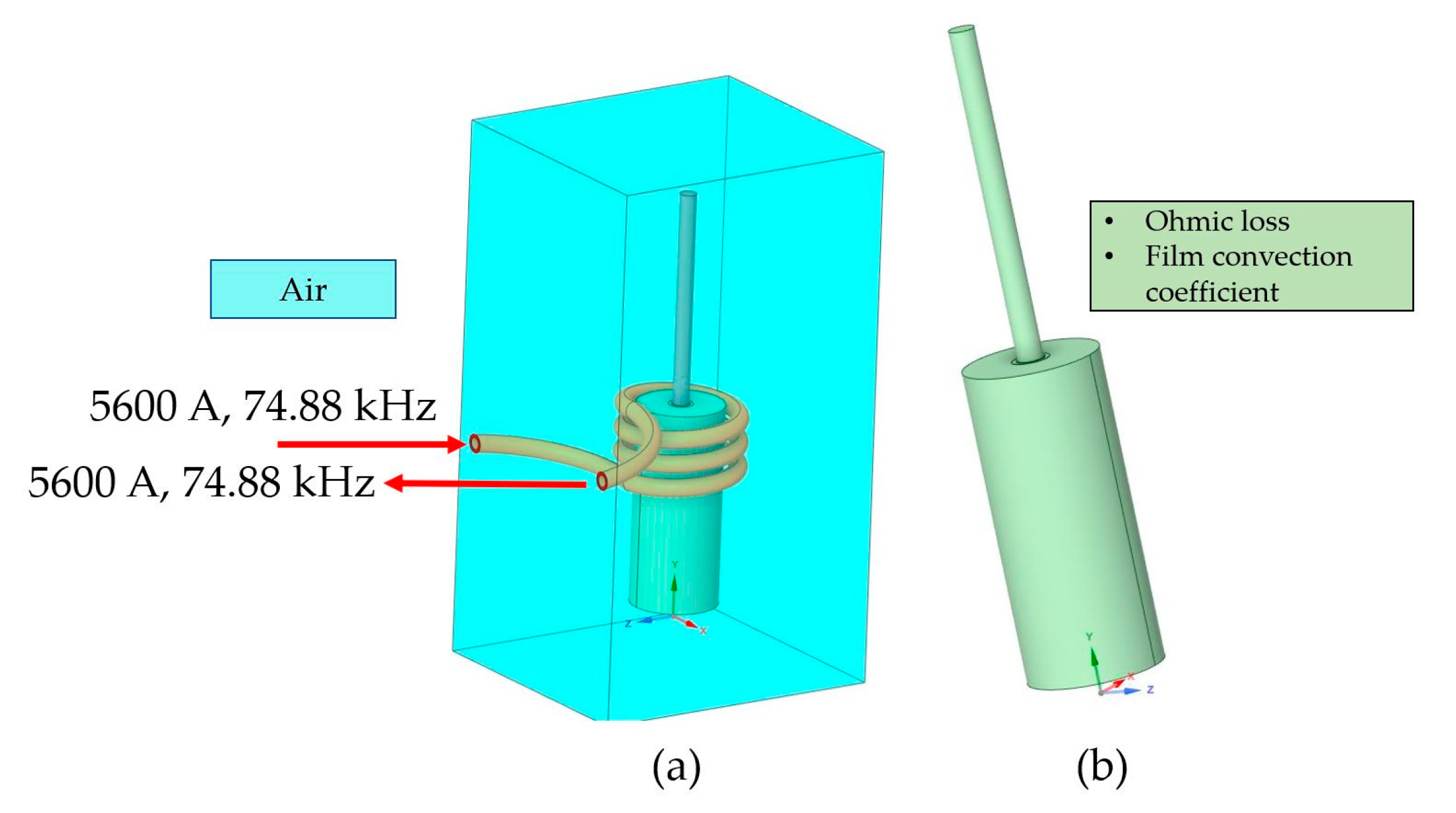
Similar to above, boundary conditions (BCs) were separated into two steps, electromagnetic and thermal simulation settings, presented in Figure 10. First, in (a) the BCs for electromagnetic simulation, the applied current (I2) of 5600 A and frequency (f) of 74.88 kHz measured in experiment #1 were set to the coil end for 7 s. Then, Ansys Maxwell solved Equation (10), yielding magnetic field and ohmic loss as simulation results. Next, after defining the ohmic loss resulting from the first step and the film convection coefficients (h) measured by experiment #2 as loads on the body and surface of the product in (b), the thermal simulation solved Equation (11) to determine the temperatures, which were compared for validation with T measured in experiment #2 for validating the simulation results, discussed next.
The method to determine temperature using h mentioned here is the same method successful in [11,12,18], but altered from thermal-electric simulation in [11,12] and CFD in [18] to electromagnetic simulation in this research. The ambient temperature at the laboratory was 25 °C. Furthermore, Table 1 reports the material properties from refs. [26,27], while Table 2 reveals h from experiment #2. The animation clip that reported the temperature distribution captured by the thermal imager helped define the h included in the Supplementary Material. The hotter regions need a higher h because their energy dissipates better than that of the cooler regions. In the calculation, the BCs were updated repeatedly until the multiphysics results converged with accurate results compared to the experimental results.
4. Results and Discussion
This section includes validation, experimental results, multiphysics results, development of IHP, and limitations and future work.
4.1. Validation
Figure 11 presents the temperature distribution on the product’s surface from the top view from (a) the experiment #2 and (b) multiphysics at 7 s from the start. The yellow texts stamped on the left in (a) are data exported from the camera software, not automatically displayed on the screen, to help with the discussion. By comparing areas on the end capsule’s surface, both results confirm that the maximum temperature (Tmax) was on the end capsule’s surface, higher than the jig’s surface since the end capsule is composed of silver, which conducts heat better than a ceramic jig, as expected. On the contrary, the minimum temperature (Tmin) was at the jig’s edge and gradually enhanced towards the center. The Tmax and Tmin were 636.1 °C and 96.1 °C in (a) and approximately 605.2 °C and 87.1 °C in (b). As expected, in (b), the temperature inside the product increased to 854 °C since the inside did not affect the air convection, as discussed later in the multiphysics results, Section 4.3. The errors from both results were 4.85% and 9.36% for the Tmax and Tmin temperatures, respectively, as further discussed in Section 4.5. Both results were consistent with minor errors; therefore, the experiment, multiphysics, and research methodology employed in this research are reliable. Both results in more detail will be reported next, separately.
4.2. Experimental Results
To investigate heat transfer and understand the IHP, Figure 12 shows the temperature distribution on the product’s surface (a–g) for times 1–7 s from experiment #2. Similar to Figure 11a, the yellow texts stamped the time and Tmax evaluated by the camera software. As expected, Tmax increased with increasing time. Tmax = 636.1 °C was in the final time of the applied current, 7 s from the start. Additionally, Tmax of approximately 89.2–636.1 °C was always on the end capsule’s surface, while the temperature on the jig’s surface was lower, approximately 21.9–124.5 °C, implying that the heat was transferred from the end capsule to others, especially the jig. An animation clip to aid the discussion in Figure 12 is in the Supplementary Material.
In addition, the ceramic jig temperature was gradually enhanced with time and had Tmax = 124.5 °C, as marked in (g), meaning that the electromagnetic field rarely affects the jig temperature since the ceramic is a good insulator, consistent with the physics principle. Using Equation (7), the skin depth (δ) of the end capsule is 0.26 mm, while the jig δ is 1853.40 mm. As a result, δ the jig is 7074 times higher than the end capsule, implying that the jig temperature entirely resulted from the heat transfer from the end capsule, and was not affected by the electromagnetic wave, as also expected. Another meaning is that electromagnetic waves can pass through the jig but only slightly penetrate the end capsule surface with 0.26 mm of its 1.0 mm thickness. Accordingly, defining multiphysics as a one-way simulation, starting with electromagnetic simulation and then transferring to thermal simulation, is reasonable. In addition, using the ceramic jig is an insulation method that is frequently used at high temperatures to reduce heat losses and increase the power required by the generator.
Unfortunately, Figure 12 cannot reveal the heat transfer and magnetic field generated by the coil, including the solder temperature inside, to ensure whether the solder was melted or not. Thus, multiphysics can help with this, as reported next.
4.3. Multiphysics
Figure 13 shows the temperature distribution inside the product at 7 s from multiphysics with thermal simulation. A small picture on the left presents an overview, while a big one on the right reveals a focusing region. A T within 340–854 °C for the end capsule and chain assures that both were not melted or damaged since the melting point for the 90% silver is 870 °C. Significantly, T was approximately 710–816 °C for the solder, close to its melting point of 70% silver at 779 °C, implying that it was melted. The small error of calculating 710 °C, lower than the melting point for the solder, may come from the limitations explained later in Section 4.5. In addition, the jig temperature was 70–849 °C, gradually decreasing from inside to outside, as expected. Therefore, the ceramic jig is not only employed for holding the product but also helps to distribute heat gradually around the product surface. From the author’s experience in the actual testing in the laboratory, without the ceramic jig, the product was burnt and damaged. Accordingly, using this operating condition, 5600 A, 74.88 kHz, and 7 s for this IHP, the heat transfer is sufficient for melting the solder without damaging the end capsule. Additionally, it is now a suitable operating condition for this product type. However, using other operating conditions may be unsuitable for heat transfer, resulting in defects. If the factory needs other operating conditions or changes in product type, multiphysics with additional experiments should be implemented to avoid any defects.
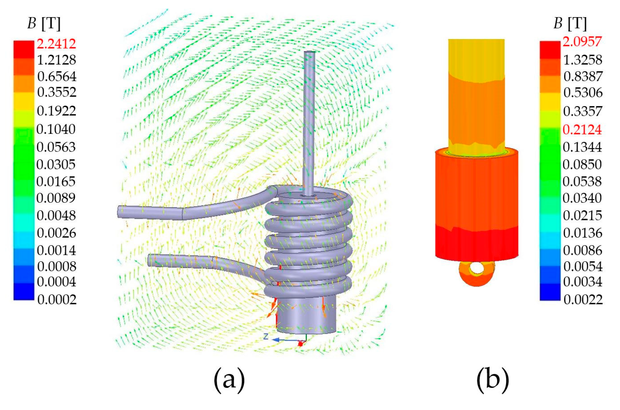
Since the coil generated the magnetic field, leading to heat transfer, as described in Section 2, understanding the relationship between both will help to develop IHP suitably. Therefore, Figure 14 reveals the coil’s magnetic flux density (B) generated, presented more in-depth in Figure 13 with the number of coil turns (N) of 3: (a) an overview as a vector plot and (b) around the product as a contour plot. In (a), this coil generated the maximum magnetic flux density (Bmax) of approximately 2.023 T, close to the coil’s surface. Away from the coil, B was reduced, as expected. Essentially, B was approximately 0.183–1.707 T, later called Brange, concentrated, and high around the product, as shown in (b), consistent with the design concept of using an induction heating machine to generate the magnetic field. Later, Bmax and Brange were used as key results to find ways to develop IHP and help with analysis. Notably, the red number in the scale bar shown in Figure 14 was used to aid analysis.
Next, the multiphysics methodology in Figure 4 was repeated to find ways to develop IHP in terms of N, product position (P), and coil thickness (Th).
- Number of Coil Turns (N)
By varying N for N = 2, 3, 4, 5, and 6, but maintaining other BC settings as the same, the multiphysics results of B were reported in Table 3. The 1st column reports N, the 2nd for the Bmax generated by N coil, and the 3rd for Brange on the product surface. In this table, Bmax reports the same results as in Figure 14a, while the Brange is compatible with Figure 14b.
From Table 3, both Bmax and Brange increase with increasing N, as expected, consistent with the Biot–Savart law of Equation (5). An example result from Table 3 is revealed in Figure 15 for N = 6, and another was included in the Supplementary Material. Comparing Figure 15 with Figure 14, both B have a similar pattern, but B increases from Bmax of 2.023 and Brange of 0.183–1.707 T in Figure 14 to Bmax of 2.241 and Brange of 0.212–2.096 T due to the increase in N. That is an increase of approximately 10.77% for Bmax and 15.85–22.79% for Brange from the coil with N =3. The more N, the higher B is. Since T increases with increasing B, confirmed by Equations (1)–(6), adding more N can reduce I2 to remain at the same level of B and T to achieve IHP.
In brief, adding more N with optimized operating conditions leads to a higher efficiency of IHP with energy savings.
- Position (P)
This aims to investigate the effect of product position and placement on B generated by the coil. Similarly, all settings remained the same with N = 3, but we reduced the vertical product position from P1 (the original placement in the factory) to P2, P3, and P4, different by 2.5 mm for each. The top surface of the product was the reference position to change. It was found that Bmax was nearly the same for all changed positions, insignificant in some, but Brange was significantly reduced. Table 4 reports the Brange calculated by multiphysics. Figure 16 shows an example for interpreting the results from Table 4; (a) changing positions and (b) B around the product at P4. Again, the Brange was reduced by reducing the vertical product position. The more the vertical product position is reduced, the lower the Brange. More in-depth, P1 in (a) is the optimum position since the product was placed in the coil center, as expected. Changing from P1 to P2, P3, and P4 shifted the product away from the center, deducting the Brange. As seen in a comparison between Figure 14b and Figure 16b, the Brange at P1 reduced from 0.183–1.707 T to 0.159–1.450 T, approximately a 13.11–15.06% reduction from the original setting. Again, red and pale red corresponded to the coil shape, with red for the near position and pale red for the far position of the coil, as expected. Other results that help with the analysis and discussion of Table 4 are included in the Supplement Material.
In brief, P1, the current position, is the optimal position for IHP. Away from P1, the efficacy of IHP declines. At P1, the optimal position for the product is in the coil center. In addition, multiphysics can be employed to determine the optimum condition of the product placement.
- Coil Thickness (Th)
Next, we aimed to investigate the effect of coil thickness (Th) on B. Again, all settings remained the same, but Th changed from the original by being increased by 40% with N = 3. Table 5 reports Bmax and Brange with a similar presentation to Table 3. The original model of the circular coil has an outer diameter of 3 mm and an inner one of 2 mm, which is 1 mm of copper thickness. From this table, increasing Th reduces both Bmax and Brange while decreasing Th enhances both, as expected. As an example result, Figure 17 reveals the B with N = 3 by decreasing 40% Th for (a) an overview and (b) around the product. A small picture on the left shows the original thickness of the coil as dashed lines, while solid lines are the thickness after reduction. Comparing Figure 17 with Figure 14, this decrease in Th by 40% (−40%) enhanced the Bmax of 2.023 T from the original model to 2.147 T, increasing 6.13%. Similarly, Brange also increases from 0.183–1.707 T to 0.184–1.721 T, increasing by approximately 0.82% around the product. Back to the theoretical background, increasing B can be explained by Equation (4). Since decreasing Th means increasing J and B relates to H, decreasing Th increases B, as expected. On the other hand, increasing Th reduces B. The bolds refer to the vector, while the italics are scalar. Additionally, other results that help with the analysis and discussion of Table 5 are included in the Supplement Material.
In brief, reducing the Th can enhance the B. Multiphysics can design the coil shape to generate more magnetic fields. However, warning, reducing Th enhances the coil temperature rapidly, leading to overheating and an unexpected shutdown of the induction heating machine. Therefore, this method required a highly efficient cooling system with proper operating conditions.
4.4. Development of IHP
From the above results presented in Section 4.3, since N, P, and Th affect B, the coil shape was optimized to achieve highly efficient IHP.
After using multiphysics by varying N, P, and Th, the optimal coil shape was N of six, P at the same position as the original model of P1, and 40% of Th decreased. Figure 18 presents the B of the optimal coil shape for (a) an overview and (b) around the product. Comparing Figure 18 with Figure 14, Bmax increased from 2.023 T to 2.342 T, approximately a 15.77% increase, and Brange from 0.183–1.707 T to 0.171–2.076 T, approximately a 21.62% increment. Since the B increases, the product’s temperature is also enhanced, as intended.
Finally, this optimal coil shape and all research findings were transferred to the factory to redesign a more efficient induction heating machine. Indeed, all reported in this article provided excellent feedback from the factory. Unfortunately, more details about the optimal coil and operating conditions implemented in the factory developed from these research findings cannot be presented because of an undisclosed agreement between the authors and the factory.
4.5. Limitations and Future Work
There are limitations since some assumptions were employed in boundary conditions, which may affect the multiphysics results and lead to errors. First, the material properties were defined as constants at a room temperature of 25 °C, although they were inconsistent depending on the temperature. Second, the coil temperature was also defined as a constant at room temperature, although it increased with continued usage. Third, I2 was defined as constant, although it fluctuated slightly with time. Fourth, the chain and end capsules were simplified to simple shapes by ignoring the factory’s unique fashion designs. Fifth, the ceramic jig was assigned to be a solid material, even though it naturally could be porous. Lastly, radiation was not taken into account in this research. However, as confirmed in Section 4.1, multiphysics results were consistent with the experimental results and theory. Accordingly, the mentioned limitations slightly affect the multiphysics results and reliability.
Due to an increase in mass production yearly, the factory required dual coils or more per induction heating machine to manufacture more necklaces promptly and continuously. Unfortunately, these research findings are based on a single coil. Fortunately, we succeeded with a reflow tip [11,12] with a dual soldering area capability that was promptly designed for a hard disk drive factory based on multiphysics. However, in the authors’ experience, heat transfers for IHP are different and complicated, requiring a deeper understanding of multiphysics settings. Since the reflow tip for the soldering process and the coil for the IHP are both based on multiphysics, applying multiphysics to the dual or more coils for the IHP based on knowledge of [11,12] is a future work for us to continue.
5. Conclusions
This article employed experiments and multiphysics consisting of electromagnetic and thermal simulations to investigate heat transfer and develop a jewelry factory’s IHP. A silver necklace with a radius of approximately 4 mm, requiring 7 s to be heated in the IHP, was employed as a case study product. First, two experiments exclusively designed and proposed in this research were set up to mimic the actual IHP to find essential parameters, such as I2, f, h, and T for validation and BC settings. Then, the essential parameters measured from the experiments were defined in multiphysics, and the simulation results revealed the heat transfer, B and T, inside and around the product. Next, T on the product surface was compared and validated with the experimental results, and the comparison confirmed that both were consistent. After that, T inside the product was validated with the theory. Again, both were consistent, assuring the reliability of multiphysics and the employing of research methodologies. The heat transfer investigation of multiphysics also revealed that T was enough to melt the solder and not damage the silver necklace’s chain and end capsule, confirming that the current operating condition was suitable; however, IHP can be improved. Later, multiphysics was applied to investigate the effect of N, P, and Th on B. As expected, they affected B, meaning that they affected T, obeying the theory. In summary, we found that increasing N enhanced B, reducing P deducted B, and reducing Th raised B. Accordingly, optimizing them can enhance B, leading to the development of IHP. Finally, N, P, and Th were optimized and analyzed to propose the optimal coil shape. Based on multiphysics, the optimal coil shape with a proper N of six, P at the same position, and Th of 40% decreasing yielded a 15.77% increase of Bmax and a 21.62% increment of Brange, better than the original coil under the same operating conditions. Therefore, the optimal coil shape was implemented in the new generation of induction heating machines for actual usage. The research findings and methodology were applied to the actual IHP and confirmed by engineers of the jewelry factory that can help develop IHP to achieve higher efficacy.
Supplementary Materials
The following supporting information can be downloaded at: https://0-www-mdpi-com.brum.beds.ac.uk/article/10.3390/pr11030858/s1. The additional results supporting Tables S3–S5 and the animation clip help defines the h and validates T, are included in the Supplementary Materials.
Author Contributions
Conceptualization, T.J. and J.T.; methodology, T.J., S.P. and J.T.; software, T.J., S.P. and J.T.; validation, T.J. and J.T.; formal analysis, J.T.; investigation, J.T.; resources, T.J. and J.T.; data curation, T.J.; writing—original draft preparation, T.J. and J.T.; writing—review and editing, J.T.; visualization, T.J.; supervision, J.T.; project administration, J.T.; funding acquisition, J.T. All authors have read and agreed to the published version of the manuscript.
Funding
This research was funded by the College of Advanced Manufacturing Innovation, King Mongkut’s Institute of Technology Ladkrabang.
Data Availability Statement
Not applicable.
Acknowledgments
This research was supported by the College of Advanced Manufacturing Innovation, King Mongkut’s Institute of Technology Ladkrabang.
Conflicts of Interest
The authors declare no conflict of interest.
Nomenclatures
| AC | Alternating current |
| I2 | Applied current to the coil (A) |
| BC | Boundary condition |
| Th | Coil thickness (mm) |
| h | Convection film coefficient (W/m2-°C) |
| DC | Direct current |
| J | Electric density (A/m2) |
| f | Frequency of the alternating current (Hz) |
| IHP | Induction heating process |
| N | Number of coil turns |
| I1 | Output current generated from the induction heating machine (A) |
| P | Position placement of product |
| Brange | Range of magnetic flux density on the product surface (T) |
| B | Scalar of magnetic flux density (T) |
| Bmax | The maximum magnetic flux density generated by the coil (T) |
| T | Temperature (°C) |
| Tmax | The maximum temperature (°C) |
| Tmin | The minimum temperature (°C) |
| TR | Transformer turn ratio |
References
- GIT. Thailand Aims to Become the World’s Gem and Jewelry Trading Hub in the Next 5 Years. Available online: https://thaitextile.org/th/insign/detail.590.1.0.html (accessed on 22 December 2022). (In Thailand).
- Marinescu, L.; Boothroyd, G. Chapter 3—Theoretical Background. In Manufacturing Engineering and Materials Processing; Inductoheat Inc.: Madison Heeights, MI, USA, 2003. [Google Scholar]
- Lucía, Ó.; Maussion, P.; Dede, E.J.; Burdío, J.M. Induction Heating Technology and Its Applications: Past Developments, Current Technology, and Future Challenges. IEEE Trans. Ind. Electron. 2014, 61, 2509–2520. [Google Scholar] [CrossRef] [Green Version]
- Kranjc, M.; Zupanic, A.; Miklavcic, D.; Jarm, T. Numerical analysis and thermographic investigation of induction heating. Int. J. Heat Mass Transf. 2010, 53, 3585–3591. [Google Scholar] [CrossRef]
- Chen, J.; Zhang, M. Numerical Simulation of Electromagnetic Induction Heating in the Material Heat Treatment. Adv. Mater. Res. 2011, 291–294, 3377–3384. [Google Scholar] [CrossRef]
- Di Luozzo, N.; Fontana, M.; Arcondo, B. Modelling of induction heating of carbon steel tubes: Mathematical analysis, numerical simulation and validation. J. Alloys Compd. 2012, 536, S564–S568. [Google Scholar] [CrossRef]
- Jianliang, J.; Shuo, L.; Chouwu, Q.; Yan, P. Numerical and experimental investigation of induction heating process of heavy cylinder. Appl. Therm. Eng. 2018, 134, 341–352. [Google Scholar]
- Choi, J.; Lee, S. High-Frequency Heat Treatment of AISI 1045 Specimens and Current Calculations of the Induction Heating Coil Using Metal Phase Transformation Simulations. Metals 2020, 10, 1484. [Google Scholar] [CrossRef]
- Ahn, C.-H.; Lee, J.; Kim, D.-J.; Shin, H.-O. Development of a Novel Concrete Curing Method Using Induction Heating System. Appl. Sci. 2021, 11, 236. [Google Scholar] [CrossRef]
- Haye, E. Industrial Solutions for Inductive Heating of Steels. Master’s Thesis, Luleå University of Technology, Luleå, Sweden, 2013. [Google Scholar]
- Thongsri, J. Transient Thermal-Electric Simulation and Experiment of Heat Transfer in Welding Tip for Reflow Soldering Process. Math. Probl. Eng. 2018, 2018, 4539054. [Google Scholar] [CrossRef]
- Thongsri, J.; Jansaengsuk, T. A Development of Welding Tips for the Reflow Soldering Process Based on Multiphysics. Processes 2022, 10, 2191. [Google Scholar] [CrossRef]
- Tangsopa, W.; Thongsri, J. A Novel Ultrasonic Cleaning Tank Developed by Harmonic Response Analysis and Computational Fluid Dynamics. Metals 2020, 10, 335. [Google Scholar] [CrossRef] [Green Version]
- Tangsopa, W.; Thongsri, J. Development of an industrial ultrasonic cleaning tank based on harmonic response analysis. Ultrasonics 2019, 91, 68–76. [Google Scholar] [CrossRef] [PubMed]
- Srathonghuam, K.; Wonganu, B.; Busayaporn, W.; Thongsri, J. Vibration Analysis and Development of a Submersible Ultrasonic Transducer for an Application in the Inhibitory Activity of Pathogenic Bacteria. IEEE Access 2021, 9, 142362–142373. [Google Scholar] [CrossRef]
- Phophayu, S.; Kliangklom, K.; Thongsri, J. Harmonic Response Analysis of Tank Design Effect on Ultrasonic Cleaning Process. Fluids 2022, 7, 99. [Google Scholar] [CrossRef]
- Jansaengsuk, T.; Kaewbumrung, M.; Busayaporn, W.; Thongsri, J. A Proper Shape of the Trailing Edge Modification to Solve a Housing Damage Problem in a Gas Turbine Power Plant. Processes 2021, 9, 705. [Google Scholar] [CrossRef]
- Thongsri, J.; Srathonghuam, K.; Boonpan, A. Gas Flow and Ablation of 122 mm Supersonic Rocket Nozzle Investigated by Conjugate Heat Transfer Analysis. Processes 2022, 10, 1823. [Google Scholar] [CrossRef]
- Tikhonova, O.V.; Malygin, I.; Plastun, A. Electromagnetic calculation for induction motors of various designs by “ANSYS maxwell. In Proceedings of the 2017 International Conference on Industrial Engineering, Applications and Manufacturing (ICIEAM), Chelyabinsk, Russia, 16–19 May 2017; pp. 1–5. [Google Scholar]
- Tikhonova, O.V.; Plastun, A.T. In Electromagnetic calculation of induction motor by “ANSYS Maxwell”. In Proceedings of the 2018 IEEE Conference of Russian Young Researchers in Electrical and Electronic Engineering (EIConRus), Moscow/St. Petersburg, Russia, 29 January–1 February 2018; pp. 822–826. [Google Scholar]
- Özüpak, Y. Performing Structural Design and Modeling of Transformers Using ANSYSMaxwell. J. Brill. Eng. 2021, 2, 38–42. [Google Scholar] [CrossRef]
- Pawar, S.; Kore, S.D.; Nandy, A. Loose Coupled Simulation Method for FEA of Electromagnetic Forming of Muffler. J. Inst. Eng. 2022, 103, 83–92. [Google Scholar] [CrossRef]
- Lecture 1: Introduction to ANSYS Maxwell. In ANSYS Maxwell V16 Trainging Manual; ANSYS Inc.: Canonsburg, PA, USA, 2013.
- Thongsri, J.; Tangsopa, W.; Kaewbumrung, M.; Phanak, M.; Busayaporn, W. Derosion Lattice Performance and Optimization in Solving an End Effect Assessed by CFD: A Case Study in Thailand’s Beach. Water 2022, 14, 1358. [Google Scholar] [CrossRef]
- Lecture 6: Meshing and Mesh Operation. In ANSYS Maxwell V16 Trainging Manual; ANSYS Inc.: Canonsburg, PA, USA, 2013.
- Silver Based Material. Available online: https://www.electrical-contacts-wiki.com/index.php?title=Silver_Based_Materials (accessed on 22 December 2022).
- Alumina (Al2O3)-CeramAloxTM. Available online: https://precision-ceramics.com/materials/alumina/ (accessed on 22 December 2022).
Figure 1.
Gold and silver necklaces manufactured from the IHP of a jewelry factory.

Figure 2.
The equipment for heat induction, including currents and magnetic fields viewed from (a) the side and (b) the top.
Figure 2.
The equipment for heat induction, including currents and magnetic fields viewed from (a) the side and (b) the top.

Figure 3.
A 2D cross-section, material types and rough dimensions.

Figure 4.
A flowchart of methodology.

Figure 5.
A diagram of an induction heating machine.

Figure 6.
A diagram of two experiments.

Figure 7.
The thermal imager setup, (a) an overview, and (b) a sample image from the camera screen.

Figure 8.
A simplified solid model.

Figure 9.
Mesh models for (a,b) electromagnetic simulation and (c) thermal simulation.

Figure 10.
Boundary conditions for multiphysics settings: (a) an overview and (b) on the product.

Figure 11.
The temperature distribution on the product’s surface from (a) the experiment #2 and (b) the multiphysics, at 7 s from the start.
Figure 11.
The temperature distribution on the product’s surface from (a) the experiment #2 and (b) the multiphysics, at 7 s from the start.

Figure 12.
The temperature distribution on the product’s surface (a–g) for times of 1–7 s from experiment #2.
Figure 12.
The temperature distribution on the product’s surface (a–g) for times of 1–7 s from experiment #2.

Figure 13.
The temperature distribution inside the product at 7 s.

Figure 14.
The magnetic flux density (B) with N = 3 for (a) an overview and (b) around the product.

Figure 15.
The magnetic flux density (B) with N = 6 for (a) an overview and (b) around the product.

Figure 16.
(a) Changing positions and (b) B around the product at P4.

Figure 17.
The magnetic flux density (B) with N = 3 by decreasing 40% Th for (a) an overview and (b) around the product.
Figure 17.
The magnetic flux density (B) with N = 3 by decreasing 40% Th for (a) an overview and (b) around the product.

Figure 18.
The magnetic flux density (B) of the optimum coil shape for (a) an overview and (b) around the product.
Figure 18.
The magnetic flux density (B) of the optimum coil shape for (a) an overview and (b) around the product.


Table 1.
Material properties (data from refs. [26,27] and the manufacturer at room temperature of 25 °C).
| Material | εr | kr | σ (S/m) | ρ (kg/m3) | Isotropic Thermal Conductivity (W/m °C) | Specific Heat (J/kg °C) |
|---|---|---|---|---|---|---|
| Jig | 9.8 | 1 | 0 | 3960 | 45 | 880 |
| Coil | 1 | 0.99991 | 58 × 106 | 8933 | 400 | 385 |
| End capsule | 1 | 0.99998 | 50 × 106 | 10,400 | 385 | 235 |
| Solder | 1 | 0.99998 | 48 × 106 | 10,000 | 325 | 235 |
| Air | 1.0006 | 1.0000004 | 0 | 1.16 | 0.03 | 1000 |
Table 2.
The film convection coefficient (data from experiment #2).
| Material | h (W/m2 °C) |
|---|---|
| Chain and End cap | 30,000–55,000 |
| Solder | 55,000 |
| Jig | 350–25,000 |
Table 3.
The Bmax and Brange by multiphysics for the various number of coil turns (N).
| N | Bmax (T) | Brange (T) |
|---|---|---|
| 2 | 1.782 | 0.139–1.293 |
| 3 | 2.023 | 0.183–1.707 |
| 4 | 2.131 | 0.228–1.942 |
| 5 | 2.165 | 0.204–1.997 |
| 6 | 2.241 | 0.212–2.096 |
Table 4.
Bmax for changing the vertical product positioning placement.
| Position | Brange (T) |
|---|---|
| P1 (original) | 0.183–1.707 (Figure 14b) |
| P2 | 0.179–1.603 |
| P3 | 0.163–1.467 |
| P4 | 0.159–1.450 |
Table 5.
The Bmax and Brange by multiphysics for the various coil thickness (Th).
| Th | Bmax (T) | Brange (T) |
|---|---|---|
| Original | 2.023 | 0.183–1.707 |
| −40% | 2.147 | 0.184–1.722 |
| +40% | 1.920 | 0.148–1.695 |
Disclaimer/Publisher’s Note: The statements, opinions and data contained in all publications are solely those of the individual author(s) and contributor(s) and not of MDPI and/or the editor(s). MDPI and/or the editor(s) disclaim responsibility for any injury to people or property resulting from any ideas, methods, instructions or products referred to in the content. |
© 2023 by the authors. Licensee MDPI, Basel, Switzerland. This article is an open access article distributed under the terms and conditions of the Creative Commons Attribution (CC BY) license (https://creativecommons.org/licenses/by/4.0/).
Share and Cite
MDPI and ACS Style
Jansaengsuk, T.; Pattanapichai, S.; Thongsri, J. A Development of an Induction Heating Process for a Jewelry Factory: Experiments and Multiphysics. Processes 2023, 11, 858. https://0-doi-org.brum.beds.ac.uk/10.3390/pr11030858
AMA Style
Jansaengsuk T, Pattanapichai S, Thongsri J. A Development of an Induction Heating Process for a Jewelry Factory: Experiments and Multiphysics. Processes. 2023; 11(3):858. https://0-doi-org.brum.beds.ac.uk/10.3390/pr11030858
Chicago/Turabian StyleJansaengsuk, Thodsaphon, Sorathorn Pattanapichai, and Jatuporn Thongsri. 2023. "A Development of an Induction Heating Process for a Jewelry Factory: Experiments and Multiphysics" Processes 11, no. 3: 858. https://0-doi-org.brum.beds.ac.uk/10.3390/pr11030858
Note that from the first issue of 2016, this journal uses article numbers instead of page numbers. See further details here.