GA−BP Prediction Model for Automobile Exhaust Waste Heat Recovery Using Thermoelectric Generator

Abstract

Thermoelectric generator (TEG) has important applications in automotive exhaust waste heat recovery. The Back propagation neural network (BP) can predict the electrical generating performance of TEG efficiently and accurately due to its advantage of being good at handing nonlinear data. However, BP algorithm is easy to fall into local optimum, and its training data usually have deviation since the data are obtained through the simulation software. Both of the problems will reduce the prediction accuracy. In order to further improve the prediction accuracy of BP algorithm, we use the genetic algorithm (GA) to optimize BP neural network by selection, crossover, and mutation operation. Meanwhile, we create a TEG for the heat waste recovery of automotive exhaust and test 84 groups of experimental data set to train the GA−BP prediction model to avoid the deviation caused by the simulation software. The results show that the prediction accuracy of the GA−BP model is better than that of the BP model. For the predicted values of output power and output voltage, the mean absolute percentage error (MAPE) increased to 2.83% and 2.28%, respectively, and the mean square error (MSE) is much smaller than the value before optimization, and the correlation coefficient (R²) of the network model is greater than 0.99.

1. Introduction

Environmental pollution and energy shortage are the foremost questions in this era [1]. According to the forecast of the International Energy Agency, by 2050, the proportion of fossil energy in the power generation will be reduced to 20% [2]. Technologies of clean energy and energy recovery are urgently required. Automobile is the most widely used transportation while about 35–40% of the engine energy is discharged into the atmosphere as the exhaust waste heat [3]. The thermoelectric generator (TEG) can directly convert heat into electrical energy [4,5,6]; therefore, it has attracted wide attention on the recovery for automobile exhaust heat in the world [7,8,9,10].

The temperatures of the automobile exhaust pipe wall vary widely at different operating conditions and positions. The temperatures of the exhaust branch, sub-muffler, and main muffler are about 480 °C, 220 °C, and 60 °C, respectively [11]. The position around the sub-muffler is usually chosen as service condition to study TEG since its temperature matches the working temperature (<300 °C) of the bismuth telluride thermoelectric module (TEM) [12]. The bismuth telluride TEM has been the most widely used due to it having the best thermoelectric properties (within 300 °C temperature aera) and mature technology [13].

At present, there is more research on the waste heat recovery for the vehicle exhaust gas using TEG, including the design and optimization of construction, as well as simulation and numerical calculation of TEG. Ge et al. developed a three-dimensional numerical simulation method using COMSOL and optimized the design of a segmented thermoelectric generator through multi-objective geneti`c algorithm [14]. Chen et al. developed a piecewise thermoelectric generator system utilizing the numerical simulation method of multi-objective genetic algorithm [15]. F Selimefendigil and H F Öztop have developed a method that combines computational fluid dynamics (CFD) with neural networks to predict the generation performance of thermoelectric generators in bifurcated channels. By utilizing hybrid modes, the time required to obtain system output performance has been reduced from 6 h using CFD simulation alone to just 3 min, effectively improving the prediction efficiency of the model [16]. Based on the finite element data set, Wang et al. utilized deep learning (DL) to predict and optimize the performance of a thermoelectric generator. By optimizing 25 key features such as the geometry of the thermoelectric leg and external load resistance, they achieved a remarkable 182% increase in output power for the module [17]. Zhu et al. utilized a training set of 5000 3-D finite element simulation data sets for neural network training, which was combined with genetic algorithm. The resulting model demonstrated a prediction accuracy of 98% and achieved precise geometric design and optimization of thermoelectric conversion devices in just 40 s. This is over 1000 times faster than the traditional finite element method [18]. Ang et al. employed an artificial neural network to predict the output voltage of a thermoelectric module under varying structural parameters and working conditions, achieving an error rate of only 0.3% between the ANN-generated output voltage and measured values [19]. Kim has developed Python code that utilizes neural networks to accurately predict the performance of thermoelectric generators in diesel engine thermoelectric generation systems, with a margin of error of only 3% between predicted and actual values. These findings highlight the potential for neural networks to be utilized in the field of thermoelectric generators [20]. In the numerical calculation, the backpropagation (BP) neural network prediction model has significant application in the performance predication of TEG [21,22] because it is suitable for nonlinear data processing [23,24] like the electrical generation performance of TEG. However, research about BP algorithm of TEG have two problems that it needs to optimize. Firstly, BP algorithm itself is prone to the drawbacks of low efficiency, local optima and prolonged convergence time [25]. Secondly, the data set used for training BP model is usually obtained through some finite element simulation software, such as COMSOL and ANASYS; however, the data set is generally inaccurate compared with the results of the experiment [26,27] because the simulation process requires the specification of boundary conditions and simplification of physical property parameters for materials.

We use genetic algorithms (GA) to improve the accuracy of BP model by varying weights because GA can obtain the optimal solution by adjusting the search direction adaptively and do not need strict rules and constraints [28,29]. In addition, we design and build a TEG for the recovery of the automotive exhaust waste heat using experimental data to train the GA−BP model for circumventing the parameter deviation caused by the simulation software. The GA−BP prediction model is established based on MATLAB software platform. We compare the deviation between the prediction and experiment values of BP and GA−BP to display the improvement effect of GA−BP algorithm on the prediction accuracy.

2. TEG and Experiment Plat

A TEG is designed and produced for waste heat recovery of vehicle exhaust. The TEG can be placed around the sub-muffler in the practical application. Figure 1a shows the structure diagram of the TEG, including hot and cold ends, TEMs, and fasten structure. Following the principle of not affecting the engine, the hot end is designed as a six square steel tube to collect the heat (Figure 1b). Furthermore, the tube structure also has good space compatibility with the exhaust pipe. Four preformed holes for the sensors are designed to monitor the exhaust parameters, such as temperature and velocity of exhaust gas, in real time.

The size of every surface of the tube collector is 40 mm × 400 mm and the inner diameter of the tube is 70 mm. The cold ends use the cooling water plates connected to a constant temperature water tank. The size of the cooling water plates is consistent with the hot end. The TEMs are bismuth-telluride-based devices with a Π shape (126 pair thermoelectric legs) and the size is 25 mm × 25 mm × 3.5 mm. A total of sixty TEMs are assembled on the six hot surfaces (ten TEMs per surface). All the TEMs have serial connection to acquire the best generating performance [2]. The surface of the TEMs is coated with silicone grease to reduce thermal contact resistance. A fasten structure is designed to further improve the heat transfer efficiency by exerting pressure. The fasten structure consists of fasten plates and screws. Pressure is exerted by tightening screws and evened by the steel plates. Figure 1c presents the image of the assembled TEG.

To evaluate the generating performance of the fabricated TEG, an experimental platform is set up, as shown in Figure 2. Tube collector wall temperature was maintained from 100 to 220 °C. temperature of the sub-muffler) by three heating rods in the middle. The inlet temperature refers to the temperature of the automatic coolant, which is about 30 to 80 °C [10]. An HWS-26 electric thermostat water bath is utilized to offer cooling water for the TEG with a range of 5~99 °C. A water pump is set to adjust the flow velocity; a PE tube Hall liquid flow meter is used to measure the velocity of cooling water within a range of 0.5–4.5 L/min. Some thermocouples are placed on the pipe wall and cooling water plate, and a TP700 multi-channel data logger is used to monitor the temperature of the hot and cold ends of the TEG at different experiment conditions. A DC electronic load meter (IT8512B+, with a maximum range of 500 V/15 A/300 W) is used for testing the open circuit voltage, electric current, and output power. The specific physical map shows Supplementary Information.

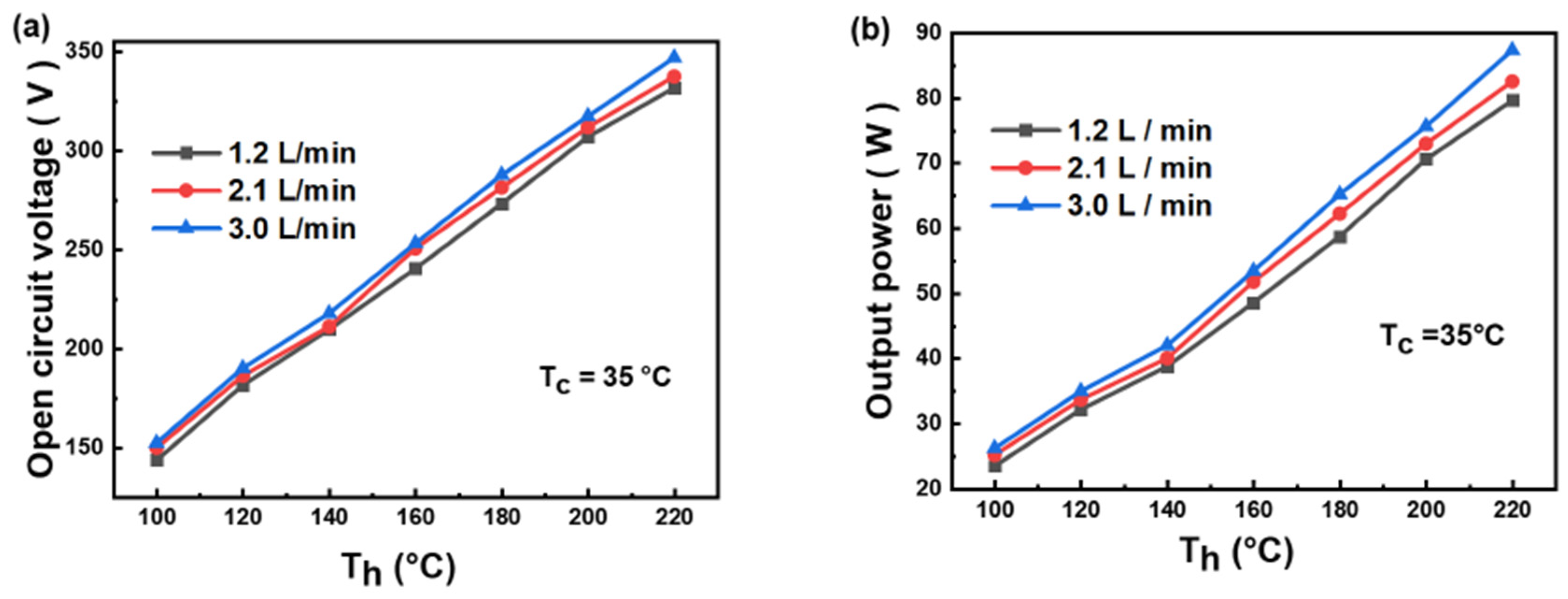
3. Experiment Results and Discussion

The temperatures of the pipe wall (T_h) and the inlet water (T_c) are the key parameters for TEG, determining the temperature difference (ΔT) established on the two ends of TEM. Figure 3 presents the open circuit voltage (OV) and output power (OP) of the fabricated TEG at different T_h and T_c in the form of 3D-surface diagram. The results are obtained based on the experiment condition of a matrix of T_h (100 °C, 120 °C, 140 °C, 160 °C, 180 °C, 200 °C, 220 °C) and T_c (35 °C, 50 °C, 65 °C, 80 °C). The water velocity (v_w) is 1.2 L/min. The results are shown in Figure 3a, OV increases with rising T_h and decreasing T_c due to the increasing ΔT on both ends of TEM. When T_h and T_c are 220 °C and 35 °C, OV reaches 331.56 V. OP is calculated according to the formula of maximum output power, as shown in Formula (1).

When the internal resistance (R_in) of the TEG is equal to the load resistance (R_L), OP of the power supply will be up to the maximum. R_in can be obtained by the Formula (2).

$$OP=\frac{{OV}^2}{{4R}_{in}}$$

(1)

$$R_{in}=\frac{OV}{I}-R_L$$

(2)

where I is the electric current corresponding to R_L and it can be tested by an amperemeter. OP is also increasing with ΔT rising, and it reaches a maximum of 79.6 W when T_h and T_c are 220 °C and 35 °C, respectively.

Besides ΔT, the water velocity (v_w) is also an influence factor for the TEG generating performance. Figure 4 presents OV and OP of TEG at different T_h (100 °C, 120 °C, 140 °C, 160 °C, 180 °C, 200 °C, 220 °C) and v_w (1.2 L/min, 2.1 L/min, 3.0 L/min); T_c is set as a fixed value of 35 °C. With the increase of T_h, the temperature difference between the ends of TEM ends becomes bigger, leading to a corresponding rise in OV and OP, and the corresponding OV and OP also increase. When the flow rate of cooling water is increased, more heat is dissipated from the cold end, resulting in a greater temperature difference and an increase in both OV and OP. OV and OP both show a rising trend with the increase in T_h and v_w since the faster water velocity can take away more heat and establish a lager temperature difference. OV and OP reach the maximum value of 346.8 V and 87.3 W when T_h is 220 °C, T_c is 35 °C and v_w is 3.0 L/min.

We collect 84 groups of experiment data of TEG at different work conditions. 60 groups of data are used to train the BP and GA−BP models, and the other 24 groups of data are used to verify the prediction results of the two algorithms. The experiment data is shown in

Table 1. Experimental data for training the GA−BP model.

Tc	Th	vw	OV	OP	Tc	Th	vw	OV	OP
35	100	1.2	143.52	23.48	65	100	1.2	88.80	12.50
35	100	2.1	149.82	25.20	65	100	2.1	91.80	13.38
35	100	3.0	152.34	26.21	65	100	3.0	92.82	14.16
35	120	1.2	181.50	32.18	65	120	1.2	125.34	18.08
35	120	2.1	186.24	33.70	65	120	2.1	130.02	19.50
35	120	3.0	190.02	34.98	65	120	3.0	131.82	20.46
35	140	1.2	209.52	38.78	65	140	1.2	162.42	25.64
35	140	2.1	211.02	40.04	65	140	2.1	168.84	28.02
35	140	3.0	217.68	42.00	65	140	3.0	171.54	29.28
35	160	1.2	240.30	48.56	65	160	1.2	202.26	35.86
35	160	2.1	250.56	51.78	65	160	2.1	208.20	37.50
35	160	3.0	253.02	53.42	65	160	3.0	211.74	39.54
35	180	1.2	273.12	58.76	65	180	1.2	239.04	44.42
35	180	2.1	281.16	62.22	65	180	2.1	245.28	47.04
35	180	3.0	287.58	65.22	65	180	3.0	249.96	49.20
35	200	1.2	306.84	70.58	65	200	1.2	275.70	56.12
35	200	2.1	311.70	72.96	65	200	2.1	287.46	60.18
35	200	3.0	317.22	75.66	65	200	3.0	293.28	65.78
35	220	1.2	331.56	79.60	65	220	1.2	314.88	70.76
35	220	2.1	337.32	82.56	65	220	2.1	323.40	73.56
35	220	3.0	346.80	87.36	65	220	3.0	328.62	76.44
50	100	1.2	112.50	15.75	80	100	1.2	66.06	9.20
50	100	2.1	113.94	17.05	80	100	2.1	67.32	10.30
50	100	3.0	114.84	18.47	80	100	3.0	69.18	11.28
50	120	1.2	143.88	21.56	80	120	1.2	107.40	14.42
50	120	2.1	144.60	22.92	80	120	2.1	111.42	15.60
50	120	3.0	145.38	24.36	80	120	3.0	112.38	16.74
50	140	1.2	175.62	28.33	80	140	1.2	134.52	18.98
50	140	2.1	177.96	29.70	80	140	2.1	138.00	20.10
50	140	3.0	179.22	31.08	80	140	3.0	140.64	21.42
50	160	1.2	213.66	38.12	80	160	1.2	185.40	30.08
50	160	2.1	216.54	39.17	80	160	2.1	190.14	31.68
50	160	3.0	218.88	40.58	80	160	3.0	193.68	33.30
50	180	1.2	252.00	47.24	80	180	1.2	222.06	39.86
50	180	2.1	261.06	49.82	80	180	2.1	231.30	43.44
50	180	3.0	267.60	53.76	80	180	3.0	233.82	44.94
50	200	1.2	291.60	61.52	80	200	1.2	258.90	52.32
50	200	2.1	295.32	64.02	80	200	2.1	265.92	55.02
50	200	3.0	303.06	67.92	80	200	3.0	271.68	56.58
50	220	1.2	326.88	74.00	80	220	1.2	309.12	62.84
50	220	2.1	334.08	77.58	80	220	2.1	317.64	65.98
50	220	3.0	341.28	81.42	80	220	3.0	325.26	67.87

.

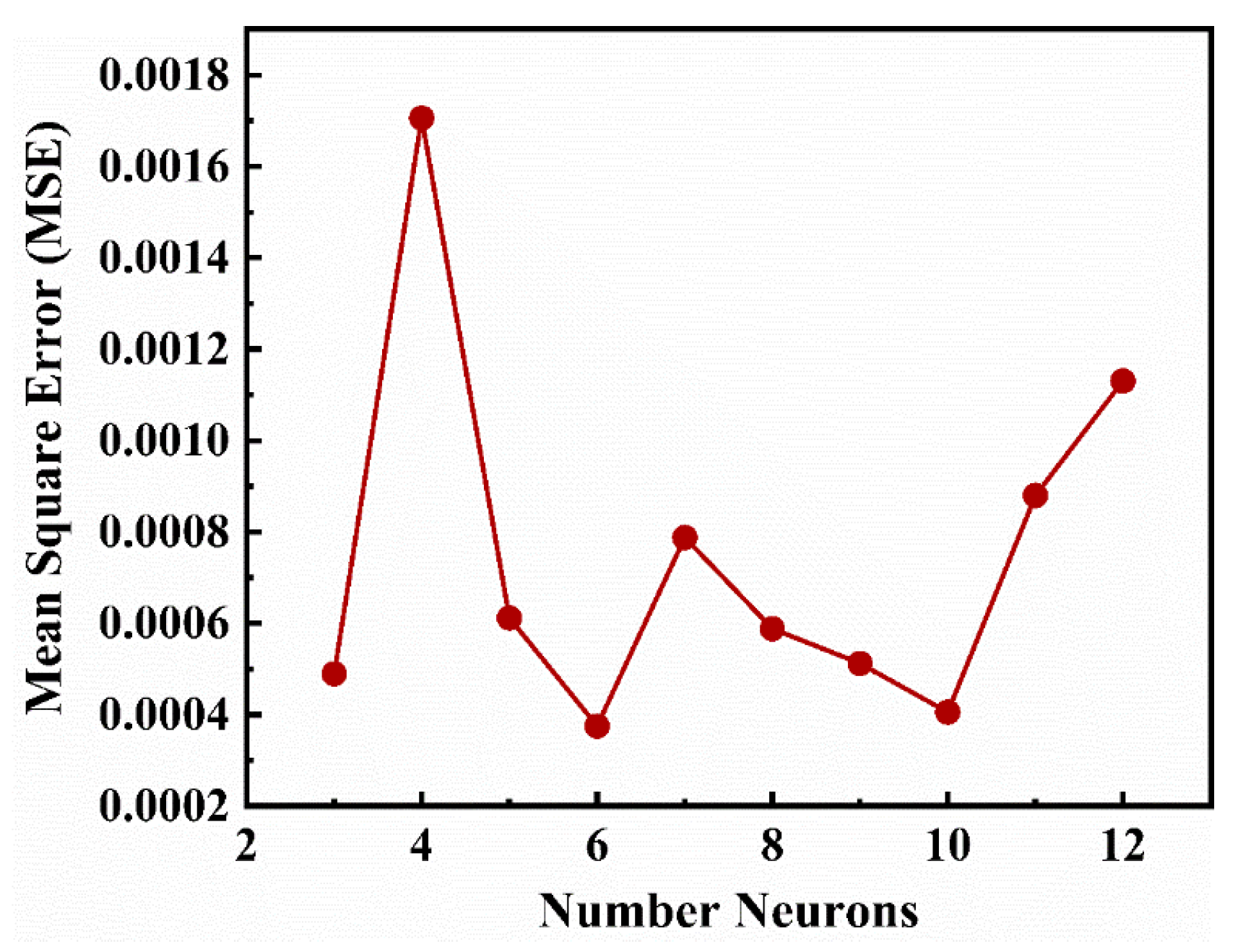
4. BP Network Model Build and Optimize

A BP neural network is built to predict the electrical generation performance of the fabricated TEG under different work conditions. BP neural network has a clear learning mechanism: signal forward propagation, error reverse transmission, memory training, and learning convergence process.

The network consists of three layers: input layer (I), implicit layer (H), and output layer (O). The layers are connected by several nodes whose states are represented by means of weights. The input layers are T_h, T_c, v_w, and the output layers are OV and OP. Figure 5 shows the training process of BP neural networks. First, information enters the hidden layer after being processed by the activation function from the input layer and then reaches the output layer after being processed by the same operation. Each neural node in the network is only affected by the node state of the upper layer. Usually, the output value obtained will produce an error from the actual value. Second, information enters the error reverse transmission stage. The error signals which do not meet the accuracy requirements, or reach the set number of iterations, will be transmitted from the output end to the input end. Meanwhile, the error value is distributed to each unit, the weight and the threshold between nodes of each layer are adjusted. After many forward and reverse transmission and learning processes, the expectant network output value is obtained though constantly adjusting and updating the weight and threshold of BP neural network. Thus, the learning process is ended.

Specific process of BP neural network modeling.

Step 1: Sample data acquisition and normalization processing. Due to different evaluation indicators, there are different dimensional units and dimensions, which will seriously affect the results of data analysis [30]. Therefore, it is necessary to standardize the data before using machine learning to analyze. Then the data analysis process is carried out with the standardized data. Commonly used bounds are [0, 1] or [−1, 1].

Step 2: The number of hidden layers and its nodes. The number of hidden layers and its nodes have great influence on the prediction accuracy of BP neural network. The excess layers will increase the computational amount and lead to a fall into the local optimum. In this work, we choose a single hidden layer considering synthetically. A small number of nodes would lead to insufficient network learning and weak training accuracy. On the other hand, a large number of nodes may cause over-fit. Thus, we use empirical formula (Equation (3)) to confirm the number of hidden layer nodes [31].

$$h=\sqrt{m+n}+a$$

(3)

where h is the number of the nodes in the hidden layer. m is the number of the input eigenvalues. n is the number of the output kind. The constant a is between 1 and 10. h is determined through comparing the testing error under different nodes numbers in the network training. The nodes number is confirmed as 6 at last (calculating results as shown in Figure 6), and the network structure is 3-6-2.

Step 3: The selection of the initial weight value, threshold value, and activation function. The input, hidden, and output layers have nodes i, k, and j (constants), respectively. The weights between the hidden, input, and output layers are defined as $w_{ik}$ and $w_{kj}$. $w_{ik}$, $w_{kj}$ and the threshold value b all use acquiescent values. Activation function adopts a Sigmoid function with good differentiability and monotonicity (S function, as shown below).

$$f\left(x\right)=\frac{1}{1+e^{-x}}x\in \left(-\mathrm{\infty },+\mathrm{\infty }\right)$$

(4)

Activation function $f$ is designed to add nonlinear factors for better treating the nonlinear TEG parameters. In addition, the learning rate and momentum factor are both 0.01, the minimum error of training target is 10⁻⁵, the training number is 1000 times.

Step 4: Signal transmission course from input layer to hidden layer. ${net}_k$ is the weight summation of the input variate at k node in hidden layer. The hidden layer output $Y_k$ is calculated according to the input training sample $x_i$, $w_{ik}$, and $b_k$ (Equation (6)).

$${net}_k=\sum _{i=1}^m{w}_{ik}·x_i+b_k$$

(5)

$$Y_k=f\left({net}_k\right) k=\mathrm{1,2},3,\cdots$$

(6)

Step 5: Signal transmission course from hidden layer to output layer. net_j is the weight summation of the input variate at j node in output layer. The prediction output $Y_j$ is obtained according to $Y_k$, $w_{kj}$, and $b_j$.

$${net}_j=\sum _{k=1}^h{w}_{kj}·Y_k+b_j$$

(7)

$$Y_j=f\left({net}_j\right) j=\mathrm{1,2},3,\cdots$$

(8)

Step 6: Calculation error. The error $e_j$ of j node in the output layer is obtained according to the prediction output value $Y_j$ and the actual value $S_j$ in the backward propagation process. $e_j=S_j-Y_j$, and E is the error function.

$$E\left(w,b\right)=\frac{1}{2}\sum _{j=1}^n{e}_j^2$$

(9)

Step 7: The errors of the weight $w_{kj}$ and threshold value $b_j$ are updated as $△w_{kj}$ and $△b_j$, as shown in follows:

$$\left[\begin{array}{c}△w_{kj}\\ △b_j\end{array}\right]=-\alpha \left[\begin{array}{c}\frac{\partial E}{\partial w_{kj}}\\ \frac{\partial E}{\partial b_j}\end{array}\right]$$

(10)

α is the learning rate. The weights and threshold values of every layer can be calculated by the following method.

$$\left[\begin{array}{c}\frac{\partial E}{\partial w_{kj}}\\ \frac{\partial E}{\partial b_j}\end{array}\right]=\frac{\partial E}{\partial e_j}·\frac{\partial e_j}{\partial Y_j}·\frac{\partial Y_j}{\partial {net}_j}·\left[\begin{array}{c}\frac{\partial {net}_j}{\partial w_{kj}}\\ \frac{\partial {net}_j}{\partial b_j}\end{array}\right]$$

(11)

After the abovementioned steps, we use the sample data to iterative learning, training, and testing.

5. GA Optimizing BP

In engineering applications, BP neural network has difficulty finding the global optimal solution because of random initial weights and thresholds while genetic algorithm (GA) has high efficiency and excellent stability, so it is regarded as an effective solution. GA is a computer simulation based on the law of “natural selection, survival of the fittest” in nature and its global random search and optimization method is obtained through the simulation of biological evolution. The four basic elements of GA algorithm are chromosome coding mode, genetic operation mode, fitness function selection, and operation parameter setting.

We use genetic algorithm to optimize BP algorithm (GA−BP). This mainly consists of three parts: first, determine the BP network; second, optimize the weight and threshold of the network by using genetic algorithm; third, network model training and prediction. In other words, the model structure is determined and remained based on the BP neural network. That is to say, the stability and efficiency of the process for searching the global optimal solution is enhanced through selection, crossover, and mutation operations, and then the optimization of the weight coefficient and threshold value is achieved [32]. The basic flow chart of GA optimization BP algorithm is shown in Figure 7.

The following is the process of GA optimizing BP prediction model.

Step 1: Population initialization. The weights and threshold value of BP neural network are coded based on the real coding. The chromosome length of the weight part and threshold part are m × h + n × h and m + n, respectively. m, h, n are the numbers of the input nodes, hidden layer nodes, and output nodes, respectively.

Step 2: Establishment of the fitness function. The fitness function (Equation (9)) represents the sum of the absolute errors between the value of the network output and actual experiment. It can distinguish the quality of the individuals in the group.

$$F=k\left(\sum _{i=1}^n\left|Y_i-S_i\right|\right)$$

(12)

where n is the number of output nodes, $Y_i$ and $S_i$ are the predicted value and the actual value of the $i$ node, and k is the coefficient.

Step 3: Selection operation. The high-fitness individuals will be selected and form a new population through the gambling method.

$$p_i=\frac{k{f}_i}{F_i{\sum }_{j=1}^N{f}_j}$$

(13)

where Fi is the individual fitness, $N$ is the number of population individuals, and $p_i$ is the probability that an individual can be selected.

Step 4: Crossover operation. The real number crossover method is selected because the individuals are encoded by real numbers. Two individuals are randomly selected from the population to perform chromosome crossover for approximating optimal solutions. The crossover operation method of j position for k chromosome A_k and l chromosome A_l is as shown in Equation (14). b is a random number between 0 and 1.

$$\left[\begin{array}{c}{A}_{kj}\\ A_{lj}\end{array}\right]=\left[\begin{array}{cc}{A}_{kj}& A_{lj}\\ A_{lj}& A_{kj}\end{array}\right]\left[\begin{array}{c}1-b\\ b\end{array}\right]$$

(14)

Step 5: Mutation operation. A better individual will be produced in this process by variation on a point of a selected individual. The operation of j gene $A_{ij}$ of i individual is as follows:

$$A_{ij}=\left\{\begin{array}{c}{A}_{ij}+(A_{ij}-A_{max})·\mathrm{f}\left(\mathrm{g}\right)\mathrm{r}\ge 0.5\\ A_{ij}+(A_{min}-A_{ij})·\mathrm{f}\left(\mathrm{g}\right)\mathrm{r}<0.5\end{array}\right.$$

(15)

where $A_{max}$ is the upper bound of gene $A_{ij}$, $A_{min}$ is the lower bound of the gene $A_{ij}$, f(g) = r₂ $\times$ (1 − g/G_max)2, $r_2$ is a random number, $\mathrm{g}$ is the current iteration number, G_max is the maximum evolution algebra, r is a random number between [0, 1]. In this paper, the initial population size is set as 30, the maximum evolutionary algebra as 100, the crossover probability P_c as 0.8, and the mutation probability P_m as 0.2.

6. Result and Discussion

In the modeling process, the mean square error (MSE) and mean absolute percentage error (MAPE) are usually used to evaluate the accuracy of the prediction model [33]. MSE can express the degree of deviation of the prediction value and experiment value. MAPE can express the percentage error of prediction results. R² can express the correlation coefficient of the network model

$$MSE=\frac{1}{n}\sum _{i=1}^N(y_i-y_i^{\prime }{)}^2$$

(16)

$$MAPE=\frac{1}{N}\sum _{i=1}^N\left|\frac{y_i-y_i^{\prime }}{y_i^{\prime }}\right|\times 100\%$$

(17)

$$R^2=1-\frac{{\sum }_{i=1}^N(y_i-y_i^{\prime }{)}^2}{{\sum }_{i=1}^N(y_i-{\stackrel{-}{y}}_i{)}^2}$$

(18)

In the formulas above, N is the number of the test samples, $y_i$ is the actual measured value, $y_i^{\prime }$ is the predicted value of the network model, and ${\stackrel{-}{y}}_i$ is the average of the actual measured values.

Figure 8 shows the iterative process of the GA−BP network. Results display that the fitness value of the optimal individual is the smallest when the iteration is about 58 times. After this process, the optimal weight and threshold are obtained and assigned to BP neural network. Figure 9 shows the convergence process of the GA−BP network. After 25 times of training, the minimum value of MSE is 0.00076, the model does not appear overfitting, and the network reaches the convergence condition.

The trained and optimized results are shown in Figure 10 through a multivariate regression analysis. The correlation coefficients R² values of the training, validation, test, and all data all exceed 0.99469, and the training R² value is up to 0.99915. These indicate that the results predicted by GA−BP model are very close to the sample data, and we obtain a reliable model.

The results of MSE and MAPE for the GA−BP prediction model are shown in

Table 2. Results of the evaluation of prediction.

Category		MSE	MAPE
OV	BP	187.85	8.50%
	GA−BP	21.36	2.28%
OP	BP	84.19	25.79%
	GA−BP	1.27	2.83%

. The prediction accuracy of GA−BP is much higher than that of BP algorithm. The MAPE can reach 2.28% (for OV) and 2.83% (for OP). The MSE are 21.36 and 1.27 for OV and OP. The assessment results further prove that the built GA−BP prediction model is reliable.

For understanding the prediction accuracy of the prediction model directly, the results of BP, GA−BP, and 24 groups of experiment data are shown in Figure 11. GA−BP model has better prediction performance compared with the BP model. Furthermore, the GA−BP model can accurately fit the OV and OP of the experiment data for the prepared TEG. The generating performance of the TEG can be accurately predicted by the GA−BP estimated in one second.

7. Conclusions

In this paper, a BP network prediction model is optimized by GA to improve the accuracy of predicting the electrical generating performance of the constructed thermoelectric generator. An experiment training dataset consisting of 84 groups is obtained to optimize the BP and GA−BP models. Of these, 60 groups are used for training the prediction model while the remaining 24 groups are utilized to verify the accuracy of GA−BP predictions. Based on the experimental results, the maximum open-circuit voltage and output power are achieved at 346.8 V and 87.3 W, respectively, when the hot end temperature is maintained at 220 °C, cold end temperature at 35 °C, and cooling water velocity at 3.0 L/min. The GA−BP model achieves a correlation coefficient R² exceeding 0.995 after training and optimization, resulting in a significantly improved prediction accuracy compared to the BP algorithm. The MAPE values for the OV and OP output parameters have significantly decreased to 2.28% and 2.83%, respectively, compared to the pre-optimization values of 8.5% and 25.79%, respectively. The MSE values for OV and OP are initially at 187.85 and 84.19 but have been reduced to only 21.36 and 1.27 after optimization, resulting in a significant decrease in error. The results collectively demonstrate that the GA−BP prediction model is highly accurate and possesses significant potential for application in TEG systems designed for vehicle exhaust waste heat recovery. Looking forward, the demand for fast and reliable TEG prediction models with exceptional performance is increasing as TEG technology continues to spread. This study can provide an experimental and theoretical basis for TEG design and numerical simulation.

References

1. Ran, Y.; Deng, Y.; Hu, T.; Su, C.; Liu, X. Energy efficient thermoelectric generator-powered localized air-conditioning system applied in a heavy-duty vehicle. J. Energy Resour. Technol. 2018, 140, 072007. [Google Scholar] [CrossRef]
2. Angeline, A.A.; Asirvatham, L.G.; Hemanth, D.J.; Jayakumar, J.; Wongwises, S. Performance prediction of hybrid thermoelectric generator with high accuracy using artificial neural networks. Sustain. Energy Technol. Assess. 2019, 33, 53–60. [Google Scholar] [CrossRef]
3. Yu, S.H.; Du, Q.; Diao, H.; Shu, G.Q.; Jiao, K. Effect of vehicle driving conditions on the performance of thermoelectric generator. Energy Convers. Manag. 2015, 96, 363–376. [Google Scholar] [CrossRef]
4. Luo, D.; Liu, Z.; Yan, Y.; Li, Y.; Wang, R.; Zhang, L.; Yang, X. Recent advances in modeling and simulation of thermoelectric power generation. Energy Convers. Manag. 2022, 273, 116389. [Google Scholar] [CrossRef]
5. Gai, X.; Wu, S.; Yang, C. Hydrothermal fluid ejector for enhanced heat transfer of a thermoelectric power generator on the seafloor. Sustain. Energy Fuels 2021, 5, 4377–4388. [Google Scholar] [CrossRef]
6. Luo, D.; Yan, Y.; Chen, W.H.; Yang, X.; Chen, H.; Cao, B.; Zhao, Y. A comprehensive hybrid transient CFD-thermal resistance model for automobile thermoelectric generators. Int. J. Heat Mass Transf. 2023, 211, 124203. [Google Scholar] [CrossRef]
7. Niu, Z.; Diao, H.; Yu, S.; Jiao, K.; Du, Q.; Shu, G. Investigation and design optimization of exhaust-based thermoelectric generator system for internal combustion engine. Energy Convers. Manag. 2014, 85, 85–101. [Google Scholar] [CrossRef]
8. Lu, C.; Wang, S.; Chen, C.; Li, Y. Effects of heat enhancement for exhaust heat exchanger on the performance of thermoelectric generator. Appl. Therm. Eng. 2015, 89, 270–279. [Google Scholar] [CrossRef]
9. Kim, T.Y.; Kwak, J.; Kim, B.W. Application of compact thermoelectric generator to hybrid electric vehicle engine operating under real vehicle operating conditions. Energy Convers. Manag. 2019, 201, 112150. [Google Scholar] [CrossRef]
10. Crane, D.; LaGrandeur, J.; Jovovic, V.; Ranalli, M.; Adldinger, M.; Poliquin, E.; Dean, J.; Kossakovski, D.; Mazar, B.; Maranville, C. TEG on-vehicle performance and model validation and what it means for further TEG development. J. Electron. Mater. 2013, 42, 1582–1591. [Google Scholar] [CrossRef]
11. Deng, Y.; Fan, T.; Guo, X.; Ling, K.; Dai, H.; Su, C. Arrangement of TEG Device and Thermoelectric Module. J. Wuhan Univ. Technol. 2010, 32, 265–267, +283. [Google Scholar]
12. Jouhara, H.; Żabnieńska-Góra, A.; Khordehgah, N.; Doraghi, Q.; Ahmad, L.; Norman, L.; Axcell, B.; Wrobel, L.; Dai, S. Thermoelectric generator (TEG) technologies and applications. Int. J. Thermofluids 2021, 9, 100063. [Google Scholar] [CrossRef]
13. Shen, Z.G.; Liu, X.; Chen, S.; Wu, S.Y.; Xiao, L.; Chen, Z.X. Theoretical analysis on a segmented annular thermoelectric generator. Energy 2018, 157, 297–313. [Google Scholar] [CrossRef]
14. Ge, Y.; Liu, Z.; Sun, H.; Liu, W. Optimal design of a segmented thermoelectric generator based on three-dimensional numerical simulation and multi-objective genetic algorithm. Energy 2018, 147, 1060–1069. [Google Scholar] [CrossRef]
15. Chen, W.H.; Chiou, Y.B. Geometry design for maximizing output power of segmented skutterudite thermoelectric generator by evolutionary computation. Appl. Energy 2020, 274, 115296. [Google Scholar] [CrossRef]
16. Selimefendigil, F.; Öztop, H.F. Thermoelectric generation in bifurcating channels and efficient modeling by using hybrid CFD and artificial neural networks. Renew. Energy 2021, 172, 582–598. [Google Scholar] [CrossRef]
17. Wang, P.; Wang, K.F.; Xi, L.; Gao, R.X.; Wang, B.L. Fast and Accurate Performance Prediction and Optimization of Thermoelectric Generators with Deep Neural Networks. Adv. Mater. Technol. 2021, 6, 2100011. [Google Scholar] [CrossRef]
18. Zhu, Y.; Newbrook, D.W.; Dai, P.; De Groot, C.; Huang, R. Artificial neural network enabled accurate geometrical design and optimisation of thermoelectric generator. Appl. Energy 2022, 305, 117800. [Google Scholar] [CrossRef]
19. Ang, Z.Y.A.; Woo, W.L.; Mesbahi, E. Artificial neural network based prediction of energy generation from thermoelectric generator with environmental parameters. J. Clean Energy Technol. 2017, 5, 458–463. [Google Scholar] [CrossRef]
20. Kim, T.Y. Prediction of System-Level Energy Harvesting Characteristics of a Thermoelectric Generator Operating in a Diesel Engine Using Artificial Neural Networks. Energies 2021, 14, 2426. [Google Scholar] [CrossRef]
21. Quan, R.; Tang, X.; Quan, S.; Huang, L. A novel optimization method for the electric topology of thermoelectric modules used in an automobile exhaust thermoelectric generator. J. Electron. Mater. 2013, 42, 1469–1475. [Google Scholar] [CrossRef]
22. Angeline, A.A. Power generation from combusted “syngas” using hybrid thermoelectric generator and forecasting the performance with ann technique. J. Therm. Eng. 2018, 4, 2149–2168. [Google Scholar] [CrossRef]
23. Wang, H.; Zhang, Z.; Liu, L. Prediction and fitting of weld morphology of Al alloy-CFRP welding-rivet hybrid bonding joint based on GA−BP neural network. J. Manuf. Process. 2021, 63, 109–120. [Google Scholar] [CrossRef]
24. Ciylan, B. Determination of output parameters of a thermoelectric module using artificial neural networks. Elektron. Ir Elektrotechnika 2011, 116, 63–66. [Google Scholar] [CrossRef]
25. Ahmadizar, F.; Soltanian, K.; AkhlaghianTab, F.; Tsoulos, I. Artificial neural network development by means of a novel combination of grammatical evolution and genetic algorithm. Eng. Appl. Artif. Intell. 2015, 39, 1–13. [Google Scholar] [CrossRef]
26. Maduabuchi, C.; Alanazi, M.; Alzahmi, A. Accurate prophecy of photovltaic-segmented thermoelectric generator’s performance using a neural network that feeds on finite element-generated data. Sustain. Energy Grids Netw. 2022, 32, 100905. [Google Scholar] [CrossRef]
27. Kishore, R.A.; Mahajan, R.L.; Priya, S. Combinatory finite element and artificial neural network model for predicting performance of thermoelectric generator. Energies 2018, 11, 2216. [Google Scholar] [CrossRef]
28. Kumar, R.R.; Dhanarajan, G.; Sarkar, D.; Sen, R. Multi-fold enhancement in sustainable production of biomass, lipids and biodiesel from oleaginous yeast: An artificial neural network-genetic algorithm approach. Sustain. Energy Fuels 2020, 4, 6075–6084. [Google Scholar] [CrossRef]
29. Yu, H.; Yin, A.; Xu, Z.; Zhang, J.; Wu, J.; Xu, X.; Zhang, Z. Grain size characterization of TA1 with GA−BP neural network using laser ultrasonics. Optik 2023, 275, 170600. [Google Scholar] [CrossRef]
30. Massaguer, A.; Massaguer, E. Faster and more accurate simulations of thermoelectric generators through the prediction of the optimum load resistance for maximum power and efficiency points. Energy 2021, 226, 120248. [Google Scholar] [CrossRef]
31. Wang, Z.; Chen, Q.; Wang, Z.; Xiong, J. The investigation into the failure criteria of concrete based on the BP neural network. Eng. Fract. Mech. 2022, 275, 108835. [Google Scholar] [CrossRef]
32. Cao, H.; Liu, L.; Wu, B.; Gao, Y.; Qu, D. Process optimization of high-speed dry milling UD-CF/PEEK laminates using GA−BP neural network. Compos. Part B Eng. 2021, 221, 109034. [Google Scholar] [CrossRef]
33. Hazare, S.R.; Patil, C.S.; Vala, S.V.; Joshi, A.J.; Joshi, J.B.; Vitankar, V.S.; Patwardhan, A.W. Predictive analysis of gas hold-up in bubble column using machine learning methods. Chem. Eng. Res. Des. 2022, 184, 724–739. [Google Scholar] [CrossRef]
Figure 1. Structure diagram of TEG (a) and the heat collection tube (b). (c) Image of TEG.
Processes 11 01498 g001
Figure 2. Schematic of Experimental system: 1. Constant temperature water tank; 2. Water pump; 3. Flowmeter; 4. Water valve; 5. Cooling water cooling plate; 6. TEM; 7. Tube Collector; 8. Thermocouple; 9. Heating rods; 10. Amperemeter. 11. Switch; 12. Voltmeter; 13. Electronic load tester.
Processes 11 01498 g002
Figure 3. The open circuit voltage (a) and output power (b) of the TEG at different pipe wall and cooling water temperature.
Processes 11 01498 g003
Figure 4. The open circuit voltage (a) and output power (b) of TEG at different pipe-wall temperature and water velocity.
Processes 11 01498 g004
Figure 5. Back Propagation neural network.
Processes 11 01498 g005
Figure 6. Variation of MSE with nodes number in the hidden layer.
Processes 11 01498 g006
Figure 7. The flow chart of GA−BP.
Processes 11 01498 g007
Figure 8. Iterative process of the genetic algorithm.
Processes 11 01498 g008
Figure 9. Convergence process of the GA−BP network.
Processes 11 01498 g009
Figure 10. Results of the multiple regression analysis for GA−BP model.
Processes 11 01498 g010
Figure 11. Comparation of OV and OP values between measurements and BP, as well as GA−BP. (a) Open Circuit Voltage; (b) Output Power.
Processes 11 01498 g011