
Numerical Analysis of Viscous Polymer Resin Mixing Processes in High-Speed Blade-Free Planetary Blender Using Smoothed Particle Hydrodynamics

Department of Mechanical and Design Engineering, Hongik University, Sejong 30016, Republic of Korea
Processes 2023, 11(9), 2555; https://0-doi-org.brum.beds.ac.uk/10.3390/pr11092555
Submission received: 4 August 2023
/
Revised: 15 August 2023
/
Accepted: 23 August 2023
/
Published: 25 August 2023
(This article belongs to the Special Issue Complex Fluid Dynamics Modeling and Simulation)
Abstract
:High-speed planetary mixers can rapidly and efficiently combine rheological liquids, such as polymer resins and paste materials, because of the large centrifugal forces generated by the planetary motion of the mixing vessel. Only a few attempts have been made to computationally model and analyze the intricate mixing patterns of highly viscous substances. This paper presents meshless flow simulations of the planetary mixing of polymeric fluids. This research utilized the smoothed particle hydrodynamics (SPH) approach for numerical calculations. This method has advantages over the finite-volume method, which is a grid-based computational technique, when it comes to modeling interfacial and free surface flow problems. Newtonian rheology and interfacial surface force models were used to calculate the dissipative forces in the partial differential momentum equation of fluid motion. Simulations of the flow of an uncured polyurethane resin were carried out while it was mixed in a planetary mixer, under various operating conditions. Simulations using SPH were able to accurately reproduce the intricate flow and blending pattern, providing insight into mixing mechanics and mixing index evolution characteristics according to operating conditions for the planetary mixing of polymeric fluids. The simulation results showed that the spiral band, which promotes the mixing performance, is densely and distinctively formed under high-speed operation conditions.
1. Introduction
The mixing of rheological substances with very high viscosity can be achieved with blade-free planetary mixers [1,2]. The typical configuration and operating conditions of a planetary mixer are shown schematically in Figure 1. A mixing vessel inclined at an angle to the horizontal plane simultaneously revolves and rotates in the opposite direction to induce a swirling motion in the substances. A high-speed planetary motion can achieve a rapid and effective mixing of viscous fluids such as viscous vesicular phospholipid gels [3], styrene-butadiene rubber dispersed with carbon nanotubes [4], and nanoscale fat emulsions [5]. Yamaga et al. [6] experimentally showed that the blade-free planetary mixing of powder-dispersed rheological material for denture relining had superior blending quality compared to conventional stir mixing in terms of mixing time, mixing homogeneity, antifoaming capacity, and the mechanical strength of the cured material.
As in the aforementioned studies, previous experimental research activities mainly focused on investigating the effectiveness of blade-free planetary mixers for the satisfactory blending of various substances that cannot be blended entirely by other types of mixer. However, they provided no experimental details for the mixing process through which insight into the planetary mixing mechanism could be obtained. This was mainly because the fluid flow measurement in a blade-free planetary mixer is very challenging. Conventional in vitro flow visualization techniques [7] such as molecular tagging velocimetry (MTV), particle image velocimetry (PIV), and laser Doppler velocimetry (LDV) are difficult to apply for planetary mixing cases due to the orbital motion of a fluid container. Current velocimetry systems are not compact enough to be attached to a moving container. To the author’s knowledge, empirical research on flow visualization in planetary mixers was published very recently in [8]. The authors constructed an experimental apparatus to characterize the planetary mixing of silicon oil in the low revolution speed range (less than 60 rpm) by applying three flow visualization techniques: particle concentration imaging, planar PIV, and tracer particle tracking. They concluded that an optimum rotation-to-revolution speed range exists for planetary mixing associated with flow separation due to chaotic advection.
Despite a lack of experimental data, a few numerical studies have been undertaken to investigate planetary mixing processes and the performance of powders and fluids. Their computational results have revealed that the performance of planetary mixers strongly depends on the operating conditions, i.e., the revolution and rotation speeds [9,10,11]. The computational work in [9] reported that the homogeneous blending of cohesive powder materials could only be achieved with planetary mixers at or above critical rotation and revolution speeds. It also showed that a faster speed and higher rotation-to-revolution ratio tend to demonstrate more effective blending of cohesive powders. The discrete element method used in [9], unlike the computational fluid dynamics (CFD) approach adopted in [10,11], can simulate the formation and dynamic evolution of the free surface of a partially charged particle bed. However, it cannot model the flow of a highly viscous non-particulate rheological medium, which is the principal interest of this paper. Chergui et al. [10] carried out CFD simulations to study the effect of the rotation-to-revolution speed ratio on the vortical flow structure of a Newtonian fluid under planetary motion. However, they only investigated the flow characteristics in the planetary blender without considering its mixing capabilities. Yamagata and Fujisawa [11] numerically investigated the mixing process and performance of a blade-free planetary mixer using computational fluid dynamics (CFD). They concluded that maximum mixing performance can be achieved around the rotation-to-revolution speed rate of 0.5. However, the CFD models in [10,11] ignored the presence and complex dynamic behavior of the surface of the free fluid during the mixing process by setting the entire inner space of the mixing vessel as the fluid domain. Recently, Shen et al. [12] reported both the CFD and experimental validation of the flow characteristics of a partially filled fluid in a planetary centrifugal bioreactor. Although their study was the first numerical effort to investigate free surface flow in a planetary motion with a maximum revolution rate of 160 rpm, it did not provide direct insight into the planetary mixing performance of rheological fluid conditions at high revolution speeds of around 1000 rpm, which are typical operating conditions for industrial mixing applications.
Unlike previous studies, the uniqueness of this paper lies in the numerical investigation of the flow and mixing characteristics of a highly viscous polymer resin (approximately 20,000 times greater viscosity than water) in a high-speed planetary mixer with a revolution rate of up to 1500 rpm. The numerical method called smoothed particle hydrodynamics (SPH) was used for mixing simulations due to its computational capabilities to account for highly viscous fluid flow, Lagrangian fluid particle tracking, and the free fluid surface [13]. This paper specifically investigated the influence of operating conditions such as the revolution speed and the rotation-to-revolution speed ratio on the mixing performance of two-part adhesive resins in a blade-free planetary mixer. The transport-velocity model [14] and the free surface boundary model [15] were used to improve the stability of the calculation and the accuracy of the solution in the SPH mixing simulations.
The remaining parts of this paper are organized as follows: The next section briefly introduces the SPH theories and describes the simulation setup and model parameters. The following section presents the SPH simulation results and discussions. The last section concludes this numerical study of the high-speed planetary mixing of viscous polymer resins.
2. SPH Model and Simulation Setup
This section presents a brief introduction to SPH theories as well as detailed numerical setups for viscous resin mixing simulations.
2.1. SPH Equations and Models
Smoothed particle hydrodynamics is a nonlocal Lagrangian mesh-free method that uses a smoothing kernel function for an approximation of field functions and their mathematical operations such as differentiation and integration [16,17,18,19,20]. A continuous computational domain in SPH is discretized with a finite number of spatially dispersed Lagrangian particles. Each particle carries its associated smoothing kernel, as well as physical quantities. With this particle-based kernel representation scheme, any field function of a position vector can be approximated as with a kernel function W by
where j is the index of a neighbor particle within the support domain associated with the smoothing length h, and and are the position vector and volume of the particle j, respectively. Therefore, the kernel function W plays a role as a weighting function of in the summing process for calculating in Equation (1).
The continuity equation and the momentum equation for a weakly compressible SPH particle i can be expressed as
and
where is the density, m is the mass of the particles, is the relative velocity vector, ∇ is the gradient operator, is the dynamic viscosity, is the relative position vector, is a small number to avoid singularity during computation, is the coefficient of liquid surface tension, is the curvature of the liquid surface, and are color functions, and is the acceleration of the gravity vector [16,17,18]. The color function to identify the particle at the phase interface [17] is defined by
The smoothing kernel used in this study is a piecewise smooth quintic spline with a cut-off radius of [21], as shown below.
where .
As proposed in [14], to mitigate a tensile instability problem that may occur while performing free surface or multiphase flow simulations with SPH [22], a transport or advection velocity is used instead of to update the particle position with
where can be calculated at every time step in the following discretized form [14]:
On the right-hand side of Equation (7), the second term with the background pressure can effectively prevent particle voids due to numerical fracture in fluid stretching situations.
An artificial equation of state was adopted as a constitutive relation between the density and the pressure p in the following form:
where is the reference pressure, is the reference density, is the speed of sound in the reference state, and is the artificial adiabatic index [21].
The computation time step is determined as a minimum or lower value that satisfies four conditions, i.e., the Courant–Friedrichs–Lewy or CFL condition, the viscous condition, the body force condition, and the surface tension condition with the time criteria corresponding to each condition sequentially listed in the MIN function as below:
where is the maximum artificial speed of sound, and is the maximum speed of fluid flow [14]. In this paper, a second-order symplectic scheme was used that considers the transport velocity in Equation (7) to integrate the governing equations in Equations (2) and (3), as in [16].
In SPH numerical simulations, particle size, material modeling, and computational time significantly impact computational accuracy in general. Particle size affects spatial resolution and solution accuracy. Smaller particles enhance numerical stability and accuracy to some extent but increase computational load [23,24]. The choice of material models influences the representation of fluid flow behaviors [25]. Advanced constitutive models enhance the precision of simulations yet increase the computational requirements. The computational time affects the scale and precision of the simulation. Longer times with more solving iterations yield more accurate results but at the cost of increased computation. Therefore, a balanced consideration of these factors is vital to achieve precise SPH results efficiently.
2.2. Simulation Setup
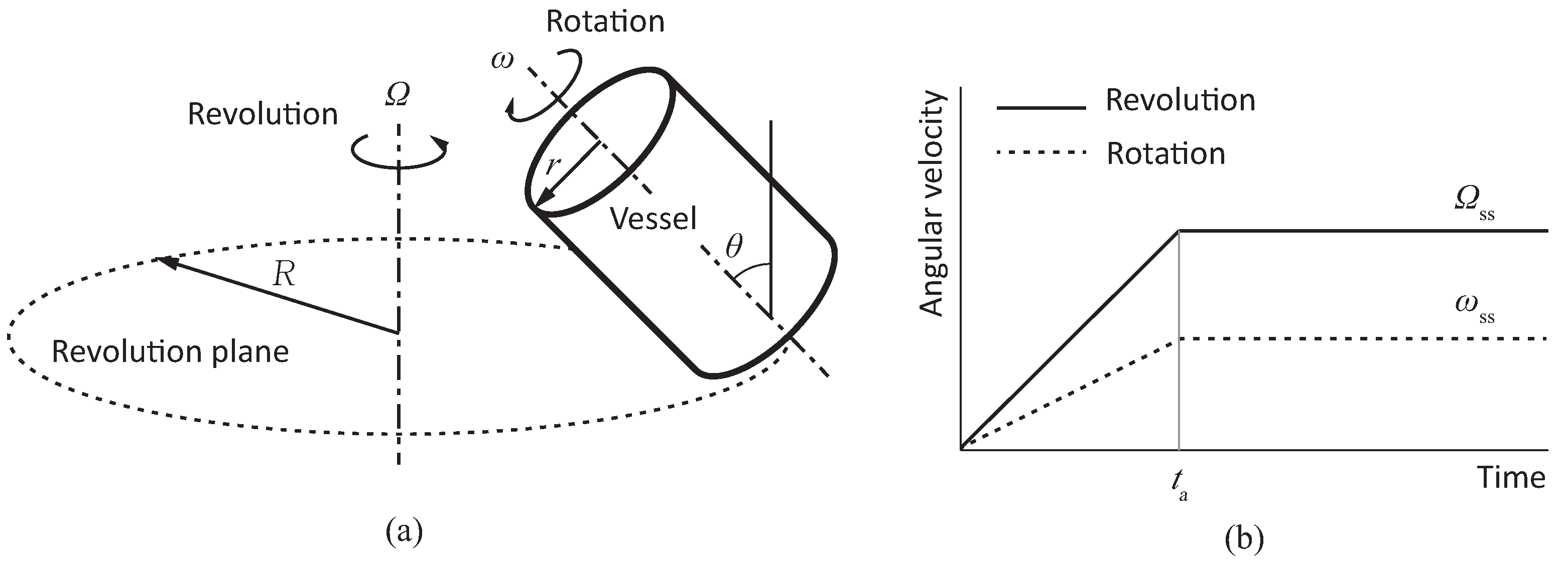
A planetary mixer, as its name implies, is a device that simultaneously applies orbital and rotational motion to the mixing vessel [10]. Figure 1a is a schematic diagram showing the planetary movement of the cylindrical vessel with an inner radius of r. The axis of rotation moves in a circular motion with a radius of R in the revolution plane. The revolution speed and the rotation speed are denoted by and , respectively. The axis of rotation is generally inclined by an angle theta with respect to the axis of revolution. The specific mixer configuration of interest in this simulation study has antidirectional revolution and rotation axes with an inclination angle of 45, which is known to exhibit optimal performance [9,26,27]. The orbital and rotational motion of the vessel starts at 0 rpm from the start time to the acceleration time , as schematically illustrated in Figure 1b, and then maintains the respective steady state speeds of and . Here, the rotation-to-revolution speed ratio is defined as n = /. In this paper, a numerical analysis study was conducted on the two-degree-of-freedom planetary mixing capable of an arbitrary combination of revolution and rotation speeds. Specifically, a total of 21 simulations were conducted with a combination of seven cases of revolution speeds (150 rpm, 300 rpm, 450 rpm, 600 rpm, 900 rpm, 1200 rpm, and 1500 rpm) and three ratios of rotation-to-revolution speed (1/3, 1/2, and 1) for each revolution speed.
The viscous polymer resin selected to perform blade-free planetary mixing simulations was a two-part epoxy adhesive (Scotch-Weld™ DP100 Plus Clear manufactured by 3M™, Two Harbors, MN, USA). This adhesive consists of a mercaptan-based accelerating hardener and an epoxy resin, denoted by part A and part B, respectively. The material properties of the hardener and epoxy resin are shown in Table 1. Regarding fluid constitutive models, the linear Newtonian viscosity models and non-Newtonian models [9,25] such as the power law model, the Bingham plastic model, and the Herschel–Bulkley model are widely used for highly viscous and rheological fluids. The maximum shear flow rate under the operating speed conditions of this paper was 39.45 s−1. A published experimental and modeling study on the rheology of uncured epoxy resin in [28] observed linearity between the shear stress and shear strain rate for a shear rate below 40 s−1, and the yield stress was very low, at about 0.2 Pa. Taking into account the small yield stress value and the stress–strain rate linearity, this numerical study appropriated the modeling of the epoxy resin fluid as a Newtonian fluid in the operating velocity regime. The mixing ratio of the two parts was 1:1 in volume, and the working time of the mixture was 4 min. When preparing a small amount of epoxy adhesive, the two parts can be easily mixed using a static mixer such as a nozzle-type inline mixer [29,30]. However, when preparing a large amount, such as for the manufacturing of epoxy matrix composite materials, a motorized resin mixer, such as a blade-free high-speed blender, should be used for complex homogeneous mixing in just a few seconds, considering both the resin working time and the material handling time [3,4].
Figure 2 shows the results of the preprocessing of the mixing vessel and the two epoxy components for the simulation of planetary mixing. The opacity of the wall particles was adjusted to 0.15 to gain a view of the fluid particles inside the container. The interior radius of the cylindrical container was 4.0 cm, the height was 8.5 cm, and the capacity was 427.3 cm3. The container was filled to a capacity of 58% with a viscous fluid, with parts A and B each comprising 29%. A rectangular knob was affixed to the top of the vessel to make it easier to observe the vessel’s rotation during the simulation. The rotation arm is a structural component for implementing planetary motion. The arm was excluded from the SPH simulation because it had no direct interaction with fluid particles. Once the original meshed CAD model was converted to SPH particles with Altair SimLab™ software version 2022.2, all particle overlaps were manually corrected. The total number of modeled particles was 52,824. Parts A, B, and the vessel comprised 15,466, 15,179, and 22,179 particles, respectively. The SPH particles were placed at an average interval of 2 mm, which was dense enough to prevent fluid particles from numerically penetrating solid walls during rapid motion.
In this study, the flow and mixing of viscous polymer resins were induced by the planetary motion of the enclosed vessel without the inlet and outlet boundaries. When the steady-state revolution velocity and the rotation-to-revolution speed ratio were both set, the operating speeds during the simulation time were determined in the form shown in Figure 1b. If the revolution speed was set to accelerate at 200 rpm per second linearly, the acceleration could be calculated as s. Assuming that the mixing vessel was a rigid body, time-series data of the vessel’s center-of-mass position and angular velocity could be generated from the angular velocity curve. The motion data were calculated and saved as an ASCII file using an in-house Python code so that an SPH solver could look up the motion data file at each computation step and update the vessel’s spatial configuration by time interpolation and numerical integration procedures.
The SPH solver adopted in this study was Altair nanoFluidX™ (or nFX for short) software version 2022.2. The nanoFluidX™ code could start a particle simulation by reading the simulation configuration file, including the numerical, domain, phase, and motion parameters. Table 2 shows the key simulation parameters defined in the configuration file. The mixing rate of each simulation case adjusted the simulation end time. The computation time step was determined to satisfy four criteria in Equation (9). The simulation result files for data visualization had a storage interval of 0.01 s.
Table 3 shows the operating conditions (steady-state revolution speed, steady-state rotation speed, and acceleration time) and the computing information (simulation time, time step size, number of iterations, and total computation time) for the 21 simulation cases. The total parallel computing time of the GPU (graphic processing unit) was 99.26 h.
3. Simulation Results and Discussion
The particle data in the SPH solver nFX were stored as a pvtu extension, which is a parallel version of the XML-based vtu (Visualization Toolkit for Unstructured Grids) file format. These vtu and pvtu files can be post-processed by an open-source Visualization Toolikt (VTK) software package version 9.3.0.RC1. The simulation data files generated for every simulation saving interval contained information on each SPH particle’s location, speed, pressure, density, and phase identification number. The results of the SPH simulation were processed and visualized using the VTK-based open-source software ParaView version 5.11.1.
Figure 3 depicts successive post-processed images at intervals of 2 s over 60 s for Case 1 ( = 150 rpm, = 50 rpm) with the lowest rotation speed among the simulation cases listed in Table 3. In the same manner as in the image processing method of Figure 2b, epoxy part A and part B were represented by red and blue spherical particles, respectively, to visually confirm the particle flow and mixing patterns. During the first 2 s of mixing, the particles maintained contact with the initial boundary surface to some extent while exhibiting a rotational flow similar to that of a rigid body. Discernible flow patterns that penetrated each other appeared on the upper free surface after 2 s and lasted for about 10 s instead of occurring on the bottom surface. After 10 s, the two fluids started to swirl and create a twisted flow pattern, causing the particle groups that were initially connected to break apart. The connectivity of the clustered fluid particles deteriorated with material convection in a whirlwind manner after 20 s. A significant breakdown of the cluster of fluid particles occurred around 50 s into the observation, resulting in an increased level of disorder and blending.
The degree of mixing of materials can be qualitatively determined by visually observing the degree of disorder in the color distribution of the particles from post-processed simulation images, like in Figure 3. However, an accurate and objective mixing level can be quantified when a quantifiable mixing index is defined and used instead of a qualitative approach. This paper adopted a mixing index that was defined as follows based on the distance between the center of gravity of the two dispersed materials [9]:
where and are, respectively, the current mass center vectors of fluid part A and part B at time t, and and are their corresponding initial position vectors.
Before operating the mixer, the mixing index in Equation (10) initially had a value of 0. Once the two materials were perfectly mixed and their centers of gravity were ideally the same, the mixing index had a value of 1. If the distance between the centers of gravity of the two materials increased during the mixing process, the mixing index could result in a negative value due to centrifugal force. Figure 4 depicts the mixing index curve of simulation Case 1, Case 2, and Case 3 with a revolution speed of 150 rpm and a rotation-to-revolution speed ratio of 1/3, 1/2, and 1, respectively. Up to about 8 s, a higher rotation-to-revolution speed ratio led to an increased rate of change of the mixing index. For n = 1, which had the highest rotation speed among the three cases, the mixing index did not increase consistently. Instead, it fluctuated after 10 s, resulting in poorer mixing compared to the other two cases. A mixing index of 80% was achieved in 11 s in all three scenarios. However, the subsequent increase in the degree of mixing was typically much slower than the initial mixing stage. Based on this analysis, the centrifugal force generated by the 150 rpm speed setting appeared to be unable to efficiently and homogeneously stir the chosen epoxy resin.
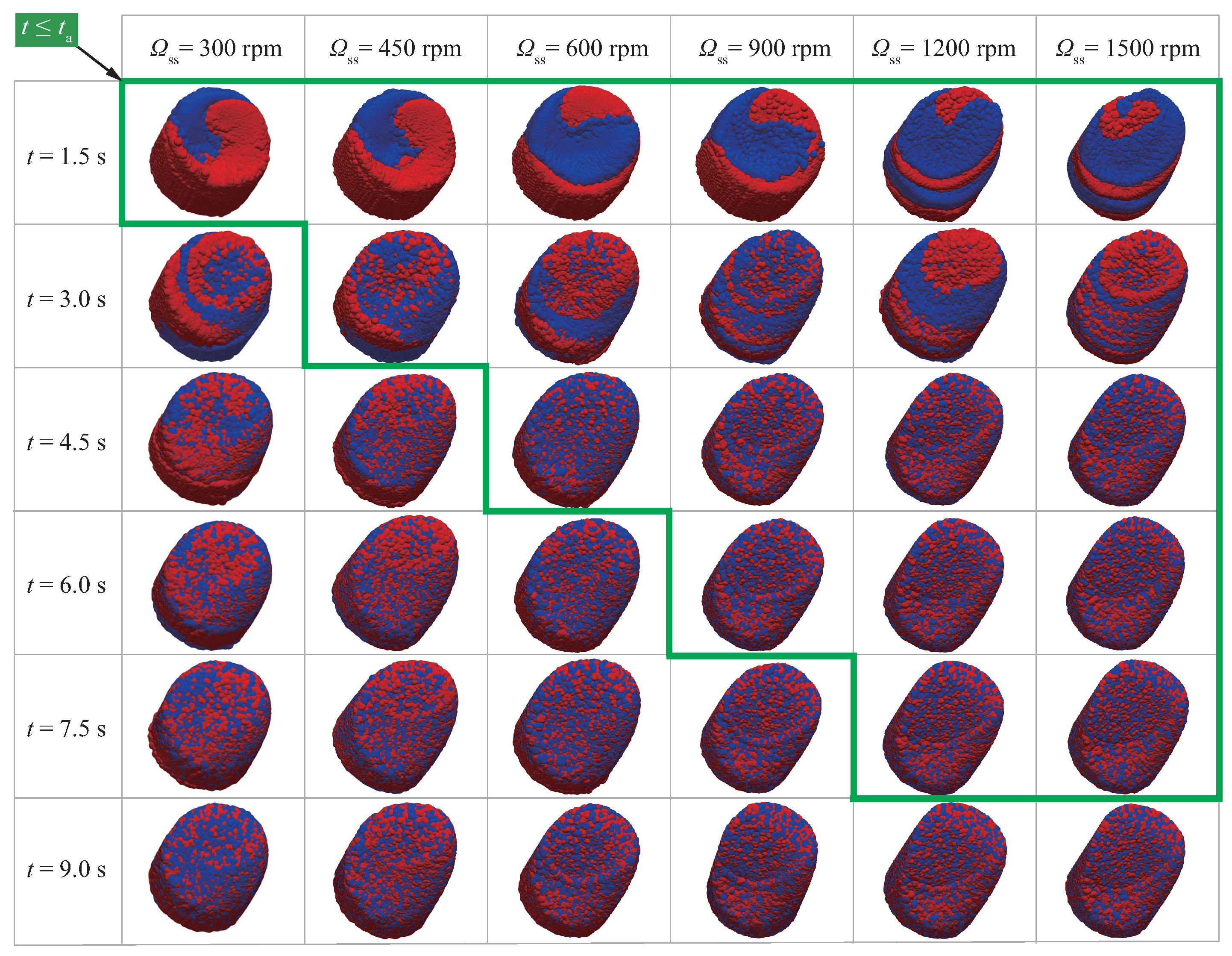
Further simulations were conducted to verify the mixing performance with the increased centrifugal forces compared to the low-speed operating conditions of 150 rpm. Eighteen simulations (Case 4–Case 21) were carried out in a range of revolution speeds of 300–1500 rpm, taking into account the range of operation speed of conventional industrial planetary mixers. Among them, the data visualization results for six cases with n = 1/3 are shown in Figure 5 at 1.5 s intervals from 1.5 s to 9 s. The thick border lines in Figure 5 indicate that the mixing vessel was in the acceleration state before reaching the steady state. Material mixing did not make significant progress during the acceleration period when < 450 rpm. On the other hand, when > 600 rpm, a noticeable improvement in material mixing was observed during acceleration. Based on the results at t = 1.5 s and t = 3.0 s, it was evident that when the revolution speed was higher, the spiral band of the fluid particles in contact with the cylindrical wall became denser and more distinct. Figure 3 shows that particle clusters separated after 50 s at 150 rpm. On the other hand, Figure 5 shows that particle segregation occurred quickly within 10 s at 300 rpm. This led to a significant enhancement in the mixing performance, depending on the operating conditions.
Figure 6 shows the time evolution curve of the mixing index for 18 simulation cases (Case 4–Case 21) in the range of revolution speeds of 300–1500 rpm. This graph comparing the mixing indices reveals three features of the rapid planetary mixing of epoxy resin. First, as the revolution speed increases, the initial slope of the mixing index curve, which represents the initial mixing rate, also increases. Second, when 900 rpm, the saturation value of the mixing index can reach nearly 100%. Third, the mixing index differences according to the rotation-to-revolution speed ratio are not significantly noticeable when 600 rpm, unlike when 450 rpm. Based on the qualitative analysis results presented in Figure 6, it has been determined that the optimal mixing performance is achieved through a combination of = 900 rpm and = 300 rpm. This combination of operating conditions results in a fast mixing time, a homogeneous resin mixture, and a low-energy consumption process.
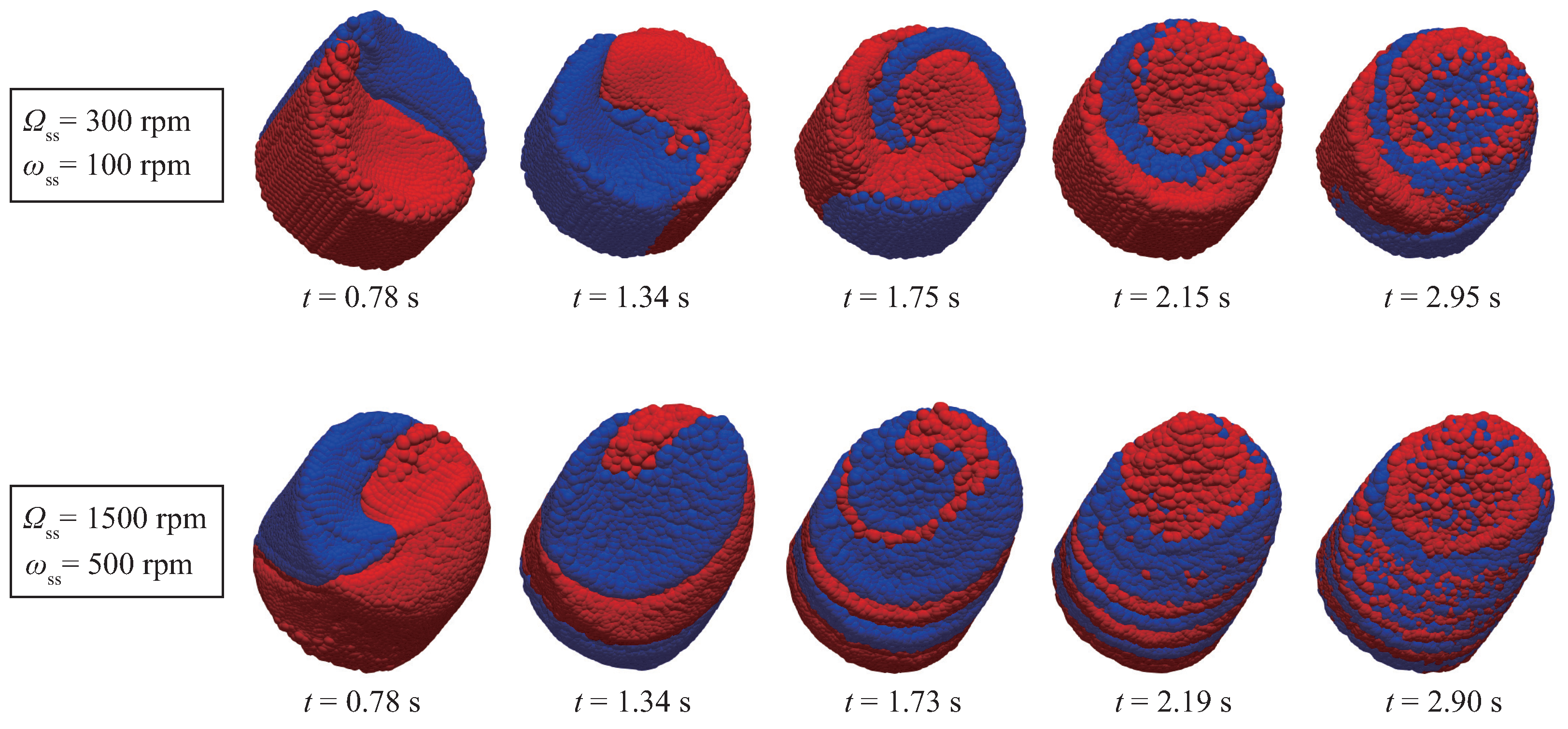
Figure 7 compares the characteristics of the initial operating phase (t < 3 s) of the low-speed ( = 300 rpm) and high-speed ( = 1500 rpm) planetary mixing situations. It can be seen that the spiral band, which promoted planetary mixing performance, was densely and distinctively formed under the high-speed operation conditions. Additionally, as seen in Figure 8, the slope and area of the upper free surface were larger in the high-speed conditions than in the low-speed conditions. Viscous fluids tend to experience faster convection as a result of the lower flow resistance on the free surface compared to the cylindrical wall surface. Therefore, the mixing performance under high-speed conditions was enhanced because of the rapid and dense formation of spiral bands on the walls, while the large free surface area allowed low-resistant fluid diffusion.
The flow characteristics and mixing states of the two viscous fluids can be observed by examining the visualized particle data presented in Figure 3 and Figure 5. Furthermore, the degree of mixing can be measured and quantified from the mixing index curves shown in Figure 4 and Figure 6. An analysis of the simulation data in Figure 3, Figure 4, Figure 5 and Figure 6 can provide insight into the influence of the operating conditions on the flow patterns, mixing mechanisms, and characteristics of mixing index evolution. Based on the simulation results, the two merit figures could be defined and used to evaluate the mixing performance, namely, the rising time and the mixing time. In this paper, the 60% rising time measures the efficiency of mixing during the initial stage before achieving uniform stirring. It is determined by the time the mixing index first reached 60%. The 90% mixing time is a performance parameter that determines how quickly a homogeneous blend can be achieved. It is defined as the minimum time required for the mixing index to remain at or above 90%.
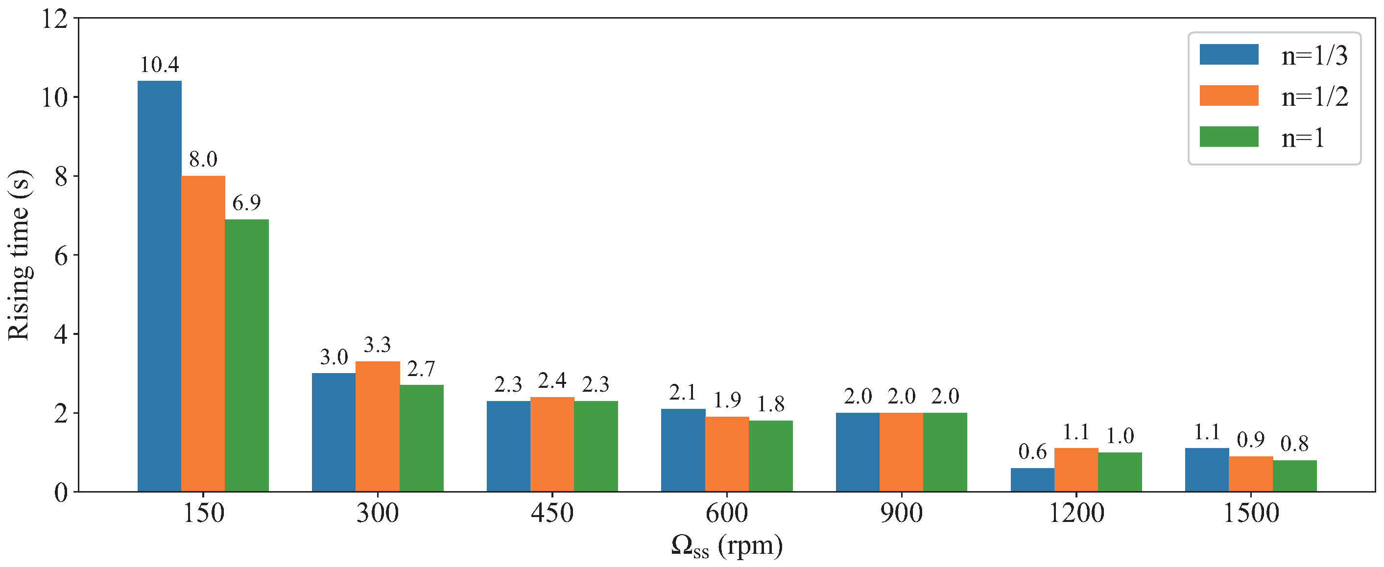
Figure 9 shows a 60% rising time bar graph extracted from the mixing index data of 21 simulation cases. At low-speed operation ( = 150 rpm), the rising time exceeded 6 s. However, it significantly improved to less than 3 s when operating at a high speed ( 300 rpm). When driving at 1200 rpm or higher, it was possible to achieve a swift rising time of approximately 1 s. When operating at = 150 rpm, the rising time increased as the rotation-to-revolution speed ratio increased. However, under high-speed driving conditions of 300 rpm, there was no overall consistent correlation between the rotation-to-revolution speed ratio and the rising time. It is imperative to select conditions where n = 1/3, because this would lead to significantly lower energy consumption when driving the rotary motor, as opposed to when n = 1/2 or n = 1.
The bar chart in Figure 10 displays the 90% mixing time, calculated using the mixing index data from 21 simulation cases. A minimum of 30 s of mixing was required at a low-speed setting of = 150 rpm to guarantee a uniform mixture. Under the operating conditions of 300 rpm, the mixing time could be reduced by 1/10 or more compared to the case of = 150 rpm. In particular, when the revolution velocity exceeded 900 rpm, the 90% mixing process took only 4 s or less. This made it ideal for blending epoxy adhesive within a restricted time frame and ensured a consistent mixture. The correlation between the rotation-to-revolution speed ratio and the mixing time in all simulation cases was observed to be unclear. However, it should be noted that this differed from the planetary mixing of cohesive pharmaceutical powders, which demonstrates a trend towards a decreased mixing time as the rotation-to-revolution speed ratio increases [9]. Based on the analyses of Figure 9 and Figure 10, the optimal operating parameters of the two-part epoxy adhesive could be determined as = 900 rpm and n = 1/3, corresponding to = 300 rpm, taking into account the energy consumption of the process and the adequacy of the mixing time.
4. Conclusions
This paper presents the results of an SPH simulation study conducted on a two-part epoxy adhesive system. The two substances were highly viscous fluids that demanded uniform mixing and rapid processing. The scope of this numerical research extended beyond previous studies by encompassing a high-speed revolution range of up to 1500 rpm, which was necessary to account for the operational capabilities of conventional industrial mixers. It is crucial to emphasize that the mixing vessel may not be entirely filled with the working fluids in real-world applications. Therefore, it is important to consider the free surface dynamics of partially filled fluids for SPH modeling and simulation. Planetary mixing simulations were performed for 21 cases, taking into account the revolution-to-revolution ratios of 1/3, 1/2, and 1 for each revolution speed of 150 rpm, 300 rpm, 450 rpm, 600 rpm, 900 rpm, 1200 rpm, and 1500 rpm. Post-processing and data analysis resulted in visualized simulation graphics, mixing index–time curves, and bar charts on rising and mixing times. Four key conclusions were drawn by the qualitative and quantitative analysis of the post-processed images and graphs. First, it was observed that when highly viscous resins were stirred in a high-speed planetary mixer, the particle fluid flow tended to be laminar with swirling patterns rather than chaotic. Second, as the revolution speed of the mixing vessel increased, the spiral band responsible for effective mixing occurred more quickly in a denser manner. This indicated a significant improvement in both the rising and mixing times, which ultimately resulted in better mixing performance. Third, at high-speed revolution speeds above 300 rpm, there was no consistent correlation between the rotation-to-revolution speed ratio and mixing performance, except for when operating under the low-speed conditions of 150 rpm. Fourth, to ensure the optimal mixing performance of an uncured two-part epoxy adhesive in terms of rising time, mixing time, and process energy consumption, it is imperative to use a combination of a 900 rpm revolution speed and a 300 rpm rotation speed for a given mixer configuration and vessel geometry. This study is a valuable contribution to the relevant research field, as it not only amplifies our understanding of planetary mixing mechanisms, encompassing the correlation between operating conditions and mixing performance, but also presents crucial insights into the most favorable operating conditions for high-viscosity polymeric fluids.
Funding
This research was supported by Basic Science Research Program through the National Research Foundation of Korea (NRF) funded by the Ministry of Education (No. 2022R1I1A3072008) and by the Ministry of Science and ICT (No. 2019R1F1A1056630).
Data Availability Statement
Not available.
Conflicts of Interest
The author declared no conflict of interest.
Nomenclature
| c | color function |
| reference speed of sound, m/s | |
| maximum artificial speed of sound, m/s | |
| f | any field function of a position vector |
| SPH approximation of field function f | |
| acceleration of gravity vector, | |
| h | smoothing length, m |
| m | particle mass, kg |
| M | mixing index |
| MIN | minimum function |
| n | rotation-to-revolution speed ratio |
| p | pressure, Pa |
| reference pressure, Pa | |
| background pressure, Pa | |
| r | inner radius of cylindrical vessel, m |
| position vector, m | |
| R | radius of revolution, m |
| s | normalized radial distance to smoothing length |
| t | current time, s |
| accelerating time, s | |
| mixing time, s | |
| rising time, s | |
| V | particle volume, |
| velocity vector, m/s | |
| transport or advection velocity vector, m/s | |
| maximum speed of fluid flow, m/s | |
| W | smoothing kernel function |
| Greek symbols | |
| coefficient of liquid surface tension, N/m | |
| artificial adiabatic index | |
| ∇ | gradient operator, 1/m |
| computational time step, s | |
| small number for computational singularity avodiance | |
| inclination angle of rotation axis, degrees | |
| curvature of liquid surface, 1/m | |
| dynamic viscosity, | |
| density, | |
| reference density, | |
| rotational speed, rpm | |
| steady-state rotational speed, rpm | |
| revolutionary speed, rpm | |
| steady-state revolutionary speed, rpm | |
| Abbreviations | |
| ASCII | American standard code for information interchange |
| CAD | computer-aided design |
| CFD | computational fluid dynamics |
| CFL | Courant–Friedrichs–Levy |
| CUDA | Compute Unified Device Architecture |
| GPU | graphics processing unit |
| LDV | laser Doppler velocimetry |
| MTV | molecular tagging velocimetry |
| nFX | nanoFluidX™ |
| PIV | particle image velocimetry |
| rpm | revolutions per minute |
| SPH | smoothed particle hydrodynamics |
| XML | extensible markup language |
References
- Adachi, N.; Hashiba, M.; Sakurada, O. Rheological Properties of Slurries Prepared Using a Planetary Mixer. Ceram. Int. 2004, 30, 1055–1058. [Google Scholar] [CrossRef]
- Hosur, M.; Barua, R.; Zainuddin, S.; Kumar, A.; Trovillion, J.; Jeelani, S. Effect of Processing Techniques on the Performance of Epoxy/MWCNT Nanocomposites. J. Appl. Polym. Sci. 2013, 127, 4211–4224. [Google Scholar] [CrossRef]
- Massing, U.; Cicko, S.; Ziroli, V. Dual Asymmetric Centrifugation (DAC)—A New Technique for Liposome Preparation. J. Control. Release 2008, 125, 16–24. [Google Scholar] [CrossRef]
- Tsuchiya, K.; Sakai, A.; Nagaoka, T.; Uchida, K.; Furukawa, T.; Yajima, H. High Electrical Performance of Carbon Nanotubes/Rubber Composites with Low Percolation Threshold Prepared with a Rotation–Revolution Mixing Technique. Compos. Sci. Technol. 2011, 71, 1098–1104. [Google Scholar] [CrossRef]
- Tenambergen, F.; Maruiama, C.H.; Mäder, K. Dual Asymmetric Centrifugation as an Alternative Preparation Method for Parenteral Fat Emulsions in Preformulation Development. Int. J. Pharm. 2013, 447, 31–37. [Google Scholar] [CrossRef] [PubMed]
- Yamaga, Y.; Kanatani, M.; Nomura, S. Usefulness of a Rotation–Revolution Mixer for Mixing Powder–Liquid Reline Material. J. Prosthodont. Res. 2015, 59, 71–78. [Google Scholar] [CrossRef]
- Mavros, P. Flow Visualization in Stirred Vessels: A Review of Experimental Techniques. Chem. Eng. Res. Des. 2001, 79, 113–127. [Google Scholar] [CrossRef]
- Yamagata, T.; Sugisawa, H.; Fujisawa, N. Experimental Study on Laminar Mixing in Planetary Mixer. Exp. Fluids 2021, 62, 28. [Google Scholar] [CrossRef]
- Son, K.J. A Numerical Study of the Influence of Operating Conditions of a Blade Free Planetary Mixer on Blending of Cohesive Powders. Korea-Aust. Rheol. J. 2019, 31, 15–23. [Google Scholar] [CrossRef]
- Chergui, N.; Lateb, M.; Lacroix, É.; Dufresne, L. CFD Study of Flow Dynamics in a Blade Free Planetary Mixer (BFPM)—A Qualitative Flow Study. Chem. Eng. Res. Des. 2015, 102, 100–115. [Google Scholar] [CrossRef]
- Yamagata, T.; Fujisawa, N. Effect of Rotation and Revolution on Performance of Blade-Free Planetary Mixer. J. Flow Control Meas. Vis. 2018, 7, 1–10. [Google Scholar] [CrossRef]
- Shen, B.; Zhan, X.; He, Y.; Sun, Z.; Long, J.; Yang, Y.; Li, X. Computational Fluid Dynamic Analysis of Mass Transfer and Hydrodynamics in a Planetary Centrifugal Bioreactor. Korean J. Chem. Eng. 2021, 38, 1358–1369. [Google Scholar] [CrossRef]
- Bouscasse, B.; Colagrossi, A.; Marrone, S.; Souto-Iglesias, A. SPH Modelling of Viscous Flow Past a Circular Cylinder Interacting with a Free Surface. Comput. Fluids 2017, 146, 190–212. [Google Scholar] [CrossRef]
- Adami, S.; Hu, X.Y.; Adams, N.A. A Transport-Velocity Formulation for Smoothed Particle Hydrodynamics. J. Comput. Phys. 2013, 241, 292–307. [Google Scholar] [CrossRef]
- Nair, P.; Tomar, G. An Improved Free Surface Modeling for Incompressible SPH. Comput. Fluids 2014, 102, 304–314. [Google Scholar] [CrossRef]
- Ji, Z.; Stanic, M.; Hartono, E.A.; Chernoray, V. Numerical Simulations of Oil Flow inside a Gearbox by Smoothed Particle Hydrodynamics (SPH) Method. Tribol. Int. 2018, 127, 47–58. [Google Scholar] [CrossRef]
- Adami, S.; Hu, X.Y.; Adams, N.A. A New Surface-Tension Formulation for Multi-Phase SPH Using a Reproducing Divergence Approximation. J. Comput. Phys. 2010, 229, 5011–5021. [Google Scholar] [CrossRef]
- Wang, Z.B.; Chen, R.; Wang, H.; Liao, Q.; Zhu, X.; Li, S.Z. An Overview of Smoothed Particle Hydrodynamics for Simulating Multiphase Flow. Appl. Math. Model. 2016, 40, 9625–9655. [Google Scholar] [CrossRef]
- Liu, M.B.; Liu, G.R. Particle Methods for Multi-Scale and Multi-Physics; World Scientific: Singapore, 2016. [Google Scholar] [CrossRef]
- Martínez-Herrera, G.; Cortez-González, J.; Murrieta-Dueñas, R.; Uribe-Ramírez, A.R.; Pérez-Segura, T.; Alvarado-Rodríguez, C.E. Smoothed Particles Hydrodynamics Simulations of Microbial Kinetic in a Stirred Bioreactor with Proximity Impellers. Comput. Part. Mech. 2022, 9, 1017–1029. [Google Scholar] [CrossRef]
- Morris, J.P.; Fox, P.J.; Zhu, Y. Modeling Low Reynolds Number Incompressible Flows Using SPH. J. Comput. Phys. 1997, 136, 214–226. [Google Scholar] [CrossRef]
- Xu, X.; Yu, P. A Technique to Remove the Tensile Instability in Weakly Compressible SPH. Comput. Mech. 2018, 62, 963–990. [Google Scholar] [CrossRef]
- Amicarelli, A.; Marongiu, J.C.; Leboeuf, F.; Leduc, J.; Caro, J. SPH Truncation Error in Estimating a 3D Function. Comput. Fluids 2011, 44, 279–296. [Google Scholar] [CrossRef]
- Violeau, D.; Fonty, T. Calculating the Smoothing Error in SPH. Comput. Fluids 2019, 191, 104240. [Google Scholar] [CrossRef]
- Abdolahzadeh, M.; Tayebi, A.; Omidvar, P. Mixing Process of Two-Phase Non-Newtonian Fluids in 2D Using Smoothed Particle Hydrodynamics. Comput. Math. Appl. 2019, 78, 110–122. [Google Scholar] [CrossRef]
- Takatsuka, T.; Endo, T.; Jianguo, Y.; Yuminoki, K.; Hashimoto, N. Nanosizing of Poorly Water Soluble Compounds Using Rotation/Revolution Mixer. Chem. Pharm. Bull. 2009, 57, 1061–1067. [Google Scholar] [CrossRef]
- Son, K.J. A Numerical Study of the Influence of Rheology of Cohesive Particles on Blade Free Planetary Mixing. Korea-Aust. Rheol. J. 2018, 30, 199–209. [Google Scholar] [CrossRef]
- Wang, Y.; Du, X. Nonlinear Constitutive Model of Uncured Epoxy Resin. J. Macromol. Sci. Part B 2005, 44, 177–184. [Google Scholar] [CrossRef]
- Meijer, H.E.H.; Singh, M.K.; Anderson, P.D. On the Performance of Static Mixers: A Quantitative Comparison. Prog. Polym. Sci. 2012, 37, 1333–1349. [Google Scholar] [CrossRef]
- Nyande, B.W.; Mathew Thomas, K.; Lakerveld, R. CFD Analysis of a Kenics Static Mixer with a Low Pressure Drop under Laminar Flow Conditions. Ind. Eng. Chem. Res. 2021, 60, 5264–5277. [Google Scholar] [CrossRef]
Figure 1.
(a) Schematic of revolution–rotation planetary mixer with cylindrical vessel and (b) its operational velocity–time plot.
Figure 1.
(a) Schematic of revolution–rotation planetary mixer with cylindrical vessel and (b) its operational velocity–time plot.

Figure 2.
Three-dimensional particle discretization: (a) original meshed CAD model and (b) post-processed SPH particle model.
Figure 2.
Three-dimensional particle discretization: (a) original meshed CAD model and (b) post-processed SPH particle model.

Figure 3.
Simulation graphics for Case 1 ( = 150 rpm, = 50 rpm) from 2 s to 60 s.

Figure 4.
Mixing index–time curves at revolution velocity of 150 rpm with rotation-to-revolution speed ratios of 1/3, 1/2, and 1.
Figure 4.
Mixing index–time curves at revolution velocity of 150 rpm with rotation-to-revolution speed ratios of 1/3, 1/2, and 1.

Figure 5.
Comparison of post-processed simulation images from 1.5 s to 9.0 s for six rotational velocities with rotation-to-revolution speed ratios of 1/3.
Figure 5.
Comparison of post-processed simulation images from 1.5 s to 9.0 s for six rotational velocities with rotation-to-revolution speed ratios of 1/3.

Figure 6.
Mixing index–time curves for six rotational velocities with rotation-to-revolution speed ratios of 1/3, 1/2, and 1 for each case: (a) 300 rpm, (b) 450 rpm, (c) 600 rpm, (d) 900 rpm, (e) 1200 rpm, and (f) 1500 rpm.
Figure 6.
Mixing index–time curves for six rotational velocities with rotation-to-revolution speed ratios of 1/3, 1/2, and 1 for each case: (a) 300 rpm, (b) 450 rpm, (c) 600 rpm, (d) 900 rpm, (e) 1200 rpm, and (f) 1500 rpm.

Figure 7.
Comparison of low- and high-speed blending characteristics between Case 4 ( = 300 rpm, = 100 rpm) and Case 19 ( = 1500 rpm, = 500 rpm) in terms of the results at the initial mixing stage.
Figure 7.
Comparison of low- and high-speed blending characteristics between Case 4 ( = 300 rpm, = 100 rpm) and Case 19 ( = 1500 rpm, = 500 rpm) in terms of the results at the initial mixing stage.

Figure 8.
Comparison of inclination of fluid free surfaces between Case 6 ( = 300 rpm, = 300 rpm) and Case 21 ( = 1500 rpm, = 1500 rpm) at t = 7.5 s.
Figure 8.
Comparison of inclination of fluid free surfaces between Case 6 ( = 300 rpm, = 300 rpm) and Case 21 ( = 1500 rpm, = 1500 rpm) at t = 7.5 s.

Figure 9.
Bar chart of 60% rising time for 21 simulation cases.

Figure 10.
Bar chart of 90% mixing time for 21 simulation cases.


Table 1.
Properties of 3M™ DP100 Plus Clear epoxy resin and mercaptan-based hardener.
| Property | Part A (Hardener) | Part B (Epoxy Resin) |
|---|---|---|
| Density () | 1150 | 1170 |
| Dynamic viscosity () | 19.4 | 11.1 |
| Admissible fluid compressibility | 0.01 | 0.01 |
Table 2.
SPH simulation parameters.
| Parameter | Value |
|---|---|
| Simulation end time 1 | Variable in range of 9.0–60.0 s |
| Integration time step 1 | Variable in range of 2.067–20.67 s |
| Data saving interval | 0.01 s |
| Reference velocity factor | 1.5 |
| Maximum number of iterations | 1,000,000,000 |
1 Specific parametric value for each simulation case is presented in Table 3.
Table 3.
Simulation cases and running options.
| Case No. | (rpm) | (rpm) | (s) | Simulation Time (s) | (s) | No. of Iterations | Computation Time 1 (h) |
|---|---|---|---|---|---|---|---|
| 1 | 150 | 50 | 0.75 | 60.0 | 20.67 | 2,902,832 | 5.15 |
| 2 | 150 | 100 | 0.75 | 60.0 | 20.67 | 2,902,832 | 5.12 |
| 3 | 150 | 150 | 0.75 | 60.0 | 20.67 | 2,902,832 | 5.13 |
| 4 | 300 | 100 | 1.50 | 15.0 | 10.33 | 1,451,416 | 2.57 |
| 5 | 300 | 200 | 1.50 | 15.0 | 10.33 | 1,451,416 | 2.53 |
| 6 | 300 | 300 | 1.50 | 15.0 | 10.33 | 1,451,416 | 2.55 |
| 7 | 450 | 150 | 2.25 | 15.0 | 6.890 | 2,177,124 | 3.75 |
| 8 | 450 | 300 | 2.27 | 15.0 | 6.890 | 2,177,124 | 3.72 |
| 9 | 450 | 450 | 2.25 | 15.0 | 6.890 | 2,177,124 | 3.73 |
| 10 | 600 | 200 | 3.00 | 12.0 | 5.167 | 2,322,266 | 4.00 |
| 11 | 600 | 400 | 3.00 | 12.0 | 5.167 | 2,322,266 | 3.93 |
| 12 | 600 | 600 | 3.00 | 12.0 | 5.167 | 2,322,266 | 3.95 |
| 13 | 900 | 300 | 4.50 | 9.0 | 3.445 | 2,612,549 | 4.43 |
| 14 | 900 | 600 | 4.50 | 9.0 | 3.445 | 2,612,549 | 4.45 |
| 15 | 900 | 900 | 4.50 | 9.0 | 3.445 | 2,612,549 | 4.43 |
| 16 | 1200 | 400 | 6.00 | 9.0 | 2.584 | 3,483,398 | 5.92 |
| 17 | 1200 | 800 | 6.00 | 9.0 | 2.584 | 3,483,398 | 5.88 |
| 18 | 1200 | 1200 | 6.00 | 9.0 | 2.584 | 3,483,398 | 5.92 |
| 19 | 1500 | 500 | 7.50 | 9.0 | 2.067 | 4,354,248 | 7.35 |
| 20 | 1500 | 1000 | 7.50 | 9.0 | 2.067 | 4,354,248 | 7.38 |
| 21 | 1500 | 1500 | 7.50 | 9.0 | 2.067 | 4,354,248 | 7.37 |
1 Simulations were performed on the GPU (model Quadro® P5000 manufacured by Nvidia, Santa Clara, CA, USA) with 2560 CUDA cores and 16 GB memory.
Disclaimer/Publisher’s Note: The statements, opinions and data contained in all publications are solely those of the individual author(s) and contributor(s) and not of MDPI and/or the editor(s). MDPI and/or the editor(s) disclaim responsibility for any injury to people or property resulting from any ideas, methods, instructions or products referred to in the content. |
© 2023 by the author. Licensee MDPI, Basel, Switzerland. This article is an open access article distributed under the terms and conditions of the Creative Commons Attribution (CC BY) license (https://creativecommons.org/licenses/by/4.0/).
Share and Cite
MDPI and ACS Style
Son, K.J. Numerical Analysis of Viscous Polymer Resin Mixing Processes in High-Speed Blade-Free Planetary Blender Using Smoothed Particle Hydrodynamics. Processes 2023, 11, 2555. https://0-doi-org.brum.beds.ac.uk/10.3390/pr11092555
AMA Style
Son KJ. Numerical Analysis of Viscous Polymer Resin Mixing Processes in High-Speed Blade-Free Planetary Blender Using Smoothed Particle Hydrodynamics. Processes. 2023; 11(9):2555. https://0-doi-org.brum.beds.ac.uk/10.3390/pr11092555
Chicago/Turabian StyleSon, Kwon Joong. 2023. "Numerical Analysis of Viscous Polymer Resin Mixing Processes in High-Speed Blade-Free Planetary Blender Using Smoothed Particle Hydrodynamics" Processes 11, no. 9: 2555. https://0-doi-org.brum.beds.ac.uk/10.3390/pr11092555
Note that from the first issue of 2016, this journal uses article numbers instead of page numbers. See further details here.